Deep Learning for Wind Speed Forecasting Using Bi-LSTM with Selected Features

1  Introduction

In the modern era, the electricity demand increases rapidly due to the fast development of the economy, industry and society. To satisfy the electricity demand with the supply, adequate power should be generated. When choosing the options for increasing the power generation, the renewable energy source dominates others [1,2]. Renewable energy forecasting mainly solar and wind energies have gained a lot of attention currently due to its vital impact on taking proper operational and managerial decisions in power systems [3,4]. The permanency, grid reliability, reduction of cost and risk level in the energy market is contingent on the accuracy of wind energy prediction [5]. The wind has a non-polluting and sustainable nature, so it has ample importance among other renewable energy sources. Accurate wind energy forecasting in power systems is a complicated task. In addition to the seasonal and climatic variations, the intermittent nature of the wind also becomes a hindrance to achieving the errorless forecasting of wind energy [6,7]. Hence, it also helps to reduce CO2 levels globally. The Global Wind Energy Council (GWEC) report states that around 743 GW of wind energy production helps to avoid around 1.1 billion tons of CO2 worldwide. The rise of grid-connected wind power, non-stationary and non-linearity characteristics of wind affect the stability of the power system. Hence, it becomes a challenge for the development of effective wind energy forecasting models [8].

Generally, the increase of input dimension introduces the curse of dimensionality issues which in turn imposes overfitting in the prediction model. The performance of prediction can be improved by reducing overfitting. It can be achieved by identifying the relevant features before the prediction process [9,10]. The feature selection improves the capability and reduces the complexity of the prediction model by providing only relevant features as input [11,12]. The feature selection has two categories namely, filter and wrapper feature selection. The statistical characteristics of each feature with the target feature are the key information used in filter feature selection to find relevant features [13]. On the other hand, the learning model is used as a feature evaluator in wrapper feature selection for finding an optimal subset of features. The filter feature selection works faster whereas the wrapper feature selection guarantees accurate results compared to filter methods [14]. In this research, the accurate wind speed is forecasted by using the combination of wrapper feature selection and deep learning methodologies. The Boruta wrapper feature selection is utilized to find the optimal subset of features for reducing the model complexity and reducing overfitting. The deep learning based Bi-LSTM is used to improve the wind speed forecasting performance by analyzing the uncertainty and non-linearity issues of the time series wind speed data. The remainder of the paper is structured as follows. The related works done by various researchers are explored in Section 2. The significance of Boruta feature selection, the function of LSTM, Bi-LSTM and the working procedure of the BFS-Bi-LSTM model are discussed in Section 3. The evaluation measures for showing the fitness of the model are presented in Section 4. The results of each prediction model, comparison and discussion are provided in Section 5. The paper is closed by providing a conclusion in Section 6.

2  Related Work

The research work already done by many researchers related to wind speed forecasting is explored in this section. The researchers have revealed a lot of methodologies for improving the performance of wind speed forecasting. In earlier days, wind speed forecasting was done by using physical models like numerical weather prediction [15]. Later on, the researchers utilized statistical models like ARIMA to forecast wind speed. But, it has a limitation in generalizing the non-linearity of data. After the development of an intelligent method, the uncertainty and non-linearity characteristic of wind speed is effectively analyzed using machine learning and deep learning methods [16,17]. Zhang et al. [18] presented two short-term wind speed forecasting models namely decomposition forecasting aggregation (DFA) and decomposition selection forecasting (DSF). First, the model decomposes the wind speed time series data and forms the input-output pairs. After that, the subset of the optimal feature is selected by constructing the prediction model with linear regression as the feature evaluator. All the combinations of the features are tested and the combination of features that produces the least validation error is selected as the best optimal subset of features. Finally, short-term wind speed is forecasted using a support vector machine (SVM) and artificial neural network (ANN). The recorded wind speed from three wind farms in china was utilized by the author for testing the model. The decomposition, feature construction and feature selection methodologies were utilized to enhance the input and improve the performance of forecasting. The DSF and DSA models with ANN and SVM outperformed the single ANN and SVM models. The author handled noisy and curse of dimensionality issues effectively.

Liu et al. [19] introduced a novel prediction model for wind speed using stacked denoising auto-encoder (SDAE) and LSTM with mutual information feature selection (MIFS). The model was compared against MLP, SAE and SDAE-LSTM. The result shows that the SDAE-LSTM with MIFS achieved better results than others. The feature selection reduced the complexity and improved the forecasting accuracy. The author considered the temporal dependency and enhanced the performance of wind speed forecasting. Liu et al. [20] developed a hybrid forecasting model for wind speed by combining feature selection, decomposition and group method of data handling (GMHD). The decomposition of the original wind speed was performed by using the ensemble empirical mode decomposition-sample entropy-wavelet packet decomposition (EEMD-SE-WPD). Followed by the optimization of the input features was done by using the binary-coded genetic algorithm (BGA). Finally, the GMHD network predicts the wind speed. As a result, the hybrid model achieved comparatively high accuracy than the single GMDH model.The hybrid model improved the accuracy of wind speed forecasting. Chen et al. [21] predicted the multi-period wind speed using SDAE, variance and extreme learning machine (ELM) based ensemble predictors. It handles well the random and intermittent nature of the wind energy.

Ghanbarzadeh et al. [22] utilized an artificial neural network (ANN) model for wind speed forecasting. The meteorological dataset with humidity, temperature and vapor pressure were utilized as input features. The ANN model with relative humidity, monthly mean daily air temperature and vapor pressure greatly improved the performance of wind speed forecasting compared to the ANN with relative humidity and monthly mean daily air temperature and ANN with relative humidity, monthly maximum daily air temperature and vapor pressure. The hybrid CNN-LSTM model was introduced by Ibrahim et al. [23]. The model improved the wind speed forecasting accuracy with less computational complexity compared to SVM, LSTM, convolutional neural network (CNN) and ANN. The model provides better accuracy than other models. Morovic et al. [24] developed an ANN based decision tool for wind speed early warning system using the data collected from the meteorological station. Huang et al. [25] designed the wind speed forecasting model using CNN. It forecasts three days ahead wind speed using the previous seven days’ wind speed. The CNN based forecasting outgunned the random forest, SVM, MLP and decision tree models.

Most of the researchers had predicted the wind speed using a variety of machine learning and deep learning methods like SVM, MLP, ELM, CNN and LSTM. Some researchers reduced the overfitting issue by considering the curse of dimensionality. The consideration of multiple related features to wind speed greatly helps for improving the accuracy of forecasting. But the consideration of too many features will introduce dimensionality issues. The presence of irrelevant features and the high dimension of the dataset becomes a hindrance to achieving better forecasting accuracy. The temporal dependency among the wind speed data is efficient information that strongly helps for predicting the future wind speed accurately from the history of wind speed data. Hence it also handles well the uncertainty issue. In this paper, the dimension and overfitting are reduced by using Boruta wrapper feature selection and also uncertainty and non-linearity issues are taken into consideration by analyzing well the temporal dependency among the history of wind speed data using deep learning based Bi-LSTM. The proposed BFS-Bi-LSTM model considers the uncertainty, curse of dimensionality, overfitting and non-linearity issues for improving the wind speed forecasting performance.

3  Methodology

3.1 Feature Selection

The feature selection is one of the dimensionality reduction techniques which is suitable for reducing the dimension of the time series meteorological dataset. In wind speed forecasting, it is inevitable to consider the additional meteorological data for accurate forecasting [26]. But all the meteorological data do not have equal importance in improving accuracy. Some features may dismantle the forecasting accuracy. The complexity of the learning model also increases when the size and dimension of data increase [27,28]. The irrelevant data given as input may confuse the learning model and increases the processing time [29]. To reduce the model complexity and to reduce the time taken for the learning process, the relevant features for the wind speed should be identified in advance [30]. The wrapper based Boruta feature selection is employed in this paper for reducing the dimensionality of the dataset. Boruta is a category of wrapper feature selection and it is strong in finding all relevant features. For wind speed forecasting we need to consider all the relevant features. Even missing of a single relevant feature also may affect the forecasting performance [31]. The Boruta feature selection finds all relevant features and reduces the curse of dimensionality and overfitting issues. The following section discusses the significance and working of Boruta feature selection.

3.1.1 Boruta Feature Selection

The Boruta feature selection is an advanced algorithm of random forest. The random forest calculates the importance of features by considering all the trees. It obtains the importance of each feature as the loss of accuracy imparted by random fluctuations of that feature in each tree separately. First, it calculates the loss of accuracy for each tree in the forest. Then it measures the average and standard deviation of accuracy loss [32]. Boruta utilizes the Z-score for measuring the importance of each feature. The fluctuations of mean accuracy loss of trees from the forest are considered for the calculation of the z-score. The z-score does not have a direct relationship with the statistical importance of the feature. The external reference is also utilized in Boruta for deciding the importance of the feature. Boruta creates one or more shadow copies for each real feature. Then, it builds the model using random forest regression and calculates the importance of all features including the shadow features [33]. Finally, it marks the real features as the important features when it has an importance value greater than the importance of all of its random features. The Z-score is the numerical measurement that is measured in terms of standard deviation from the mean. It may be positive or negative. Z-score is positive when the value is above the mean and it is negative when the Z-score value is below the mean. When it is equal to the mean it gets the value 0. Let the feature value is ‘x’, the mean is ‘μ’ and the standard deviation is ‘σ’. The mean is calculated as follows,

μ=∑i=1nxiN (1)

where the total number of samples is denoted as ‘N’ and each sample is denoted as ‘n’. The standard deviation and Z-score are calculated as follows,

σ=∑i=1n(xi−μ)2N (2)

Z−score = x−μσ (3)

The Boruta feature selection wraps the random forest procedure. But it is the improved version of random forest in the way that it generates the maximal subset of features. The random forest over prunes the features in each iteration and sometimes it may lead to the throwing of relevant features also. But, the Boruta finds all the weakly and strongly relevant features related to the target feature and provides an optimal subset of features.

3.2 Deep Learning for Wind Speed Forecasting

Deep learning is very useful for learning the non-linear wind speed and meteorological features to present a strong generalization. The non-linearity and uncertainty properties of wind speed are imposing complications on the learning process. An effective deep learning methodology named recurrent neural network (RNN) is adaptable for handling uncertainty and non-linearity by using the sequence dependence nature of load data [34,35]. It keeps the sequence dependence by looping back the cell state information in each hidden unit after the computation. At each time step, it utilizes the current timestep information along with past timestep information to produce output for the current timestep. It performs the recursive process of keeping the cell state information in each hidden unit itself [36,37]. However, RNN processes the time series sequence dependence data well, it is affected by the short term memory issue. The advanced version of RNN called LSTM and Bi-LSTM overcomes this issue by replacing each neuron in the hidden unit by the memory with three gates.

3.2.1 Multilayer Perceptron (MLP)

The multilayer perceptron is the deep artificial neural network that consists of many perceptrons. They are grouped in three layers namely, the input layer, hidden layer and output layer. The input layer receives the input and the output layer produces the prediction output. In between the input and output layer, several hidden layers perform the actual computation of MLP. It is a simple feed-forward artificial neural network that passes the input received at the input layer to the output layer through the hidden layers. The hidden layer neurons utilize the activation function such as tanh, sigmoid and ReLU for producing the output. It utilizes the backpropagation technique for training. After the output is produced in each hidden neuron, it is forwarded to the neurons in the next adjacent layer till reaching the output layer. Once the output is generated at the output layer the difference between the expected output and observed output is calculated to find the error. Then, this error is propagated in the backward direction from the output to the input layer and the connection weight is updated [38]. The MLP has the capability of handling well the multivariate, non-linear and regression data. So, it is utilized as one of the comparing models to show the performance of the proposed model.

3.2.2 Long Short Term Memory (LSTM)

The LSTM is a variant of simple RNN that overcomes the issues associated with it. In RNN, the gradient information may get disappeared or may explode when the number of layers increases. So, the simple RNN suffers from low learning efficiency and reverse optimization. In addition to that, it suffers from short term memory [39,40]. So, it cannot keep the hidden state information for a longer period. These issues are resolved in LSTM by utilizing the recurrently connected memory cells and gates [41,42]. The external memory is utilized to maintain the memory state over a period. The gating mechanism is utilized in each memory cell of LSTM for regulating the information flow to and from the memory cell. The forget, input and output gates decide which information is no longer required to be maintained in the cell, which information from the input should be utilized for updating the current state and which information should be included in the output respectively [43]. Instead of utilizing all the previous cell state information at the current cell as RNN, it performs the flexible selection of the information using gates. It retains information for a longer period and effectively analyses the sequence dependency of time series meteorological data [44,45].

3.2.3 Bidirectional Long Short Term Memory (Bi-LSTM)

The Bi-LSTM works well with sequence data by learning the sequences faster than the unidirectional LSTM. It also can capture the complex dependencies that exist in the sequence data easily. The structure of bidirectional LSTM is the same as that of LSTM but, it consists of the forward and reverse recurrent components for processing the data in forward and reverse directions respectively. It consists of three gates namely, forget gate, output gate and input gate. It uses the sigmoid function as the activation function in forget and output gates. It uses tanh and sigmoid functions as the activation function in the input gate. It produces the output at any time ‘t’ by considering the previous and future elements in the sequence whereas the unidirectional LSTM produces the output only depending on the previous element. The bidirectional LSTM partitions its neurons into two groups, one for passing the state information in the forward direction and another one for passing the state information in the reverse direction. So, it has two cells in each hidden node, one keeps the past value and another one keeps the future value [46,47]. The folded and unfolded bidirectional LSTM architecture is shown in Fig. 1. The bidirectional LSTM network adds more LSTM layers one on top of another to preserve the previous and future input details for a long sequence of time and flows the data in both directions. However, the output of the states in these two directions is not interconnected with each other. So, the weight update of the neurons in the input and output layers cannot be performed at the same time. During the forward pass, the forward state and backward state information are passed before forwarding it to output neurons. But, during the backward pass, the forward and backward state information are passed after passing the output neurons. The Bi-LSTM computes the forward hidden sequence first, then computes the backward hidden sequence. Finally, it generates the output by combining these two sequences.

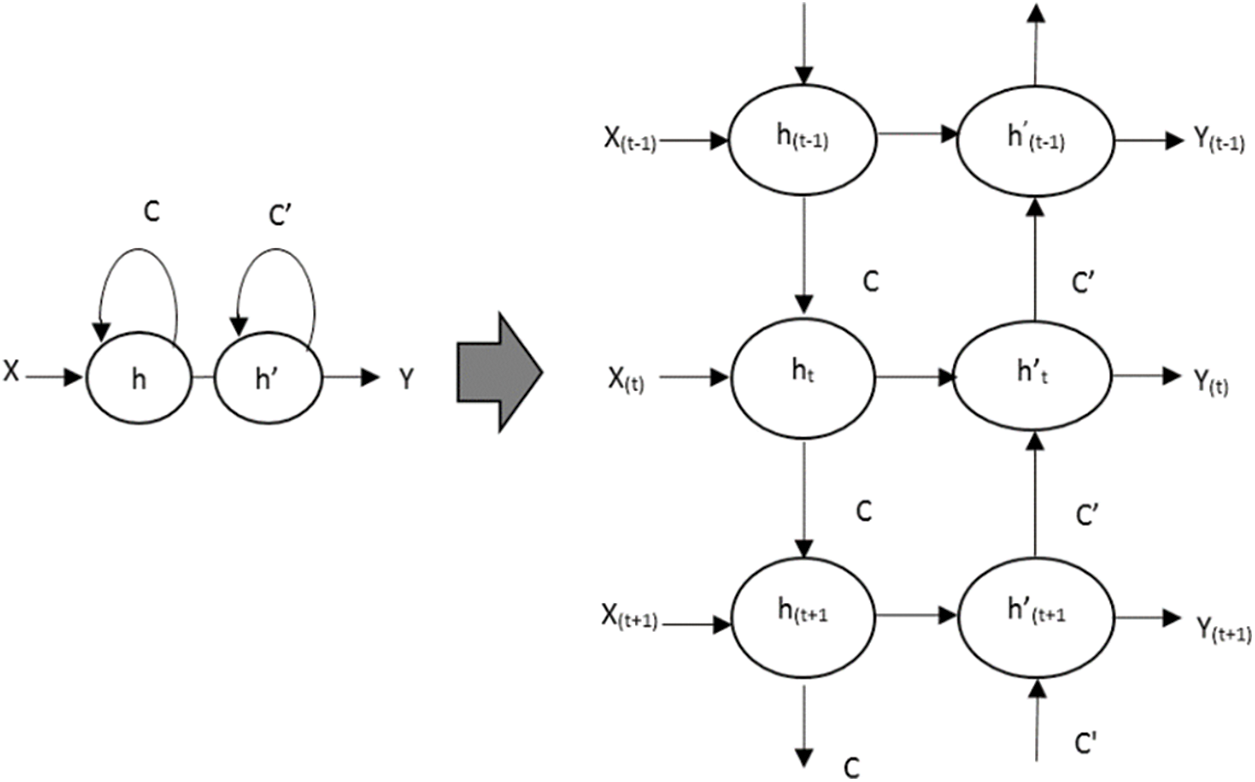
Figure 1: Folded and unfolded bidirectional LSTM

Let the input layer is represented as ‘x’, the output layer is represented as ‘y’, the hidden layer is represented as ‘h’, bias is represented as ‘b’, the weight matrix is represented as ‘w’, cell state at the forward stage is represented as ‘C’, cell state at the backward stage is represented as C’, the activation function is represented as ‘H’ and time is represented as ‘t’. The forward hidden vector sequence is generated as,

ht→=H(wxh→xt+wh→h→h→t−1+bh→) (4)

The backward hidden vector sequence h←t is generated as,

ht←=H(wxh←xt+wh←h←h←t−1+bh←) (5)

Finally, the output vector sequence is generated by combining both the forward and backward hidden vector sequences as follows,

yt=wh→yh→t+wh←yh←t+by)(6)

In this paper, the two layers of the bidirectional LSTM are introduced for processing and capturing the dependencies hidden in the longer and complex non-linear wind speed sequences.

3.2.4 Proposed BFS-Bi-LSTM Model

Significance of BFS-Bi-LSTM

In wind speed forecasting, the consideration of additional meteorological data is inevitable for accurate forecasting. But all the meteorological data do not have equal importance in improving accuracy. Some features may dismantle the forecasting accuracy. The irrelevant data in the input may baffle the learning model and increases the processing time. Even missing a single relevant feature also may affect the forecasting performance. The complexity of the learning model increases when the size and dimension of the data increase. In this paper, Boruta feature selection is utilized for reducing the complexity of the Bi-LSTM by reducing the curse of dimensionality. The temporal dependency among the wind speed data is an efficient information that strongly helps for predicting accurately the future wind speed from the history of wind speed data. Hence it also handles well the uncertainty issue. In this paper, the dimension is reduced to reduce the complexity and to enhance the accuracy by using Boruta feature selection. The uncertainty issues are also taken into consideration by analyzing well the temporal dependency among the history of wind speed data using deep learning based Bi-LSTM. The proposed BFS-Bi-LSTM model considers uncertainty, the curse of dimensionality and the temporal dependency issues and improves the wind speed forecasting performance.

BFS-Bi-LSTM Architecture

The proposed Bi-directional long short term memory with the Boruta feature selection (BFS-Bi-LSTM) is a hybrid model that is a combination of feature selection and deep learning. BFS-Bi-LSTM consists of four stages in predicting wind speed. They are preprocessing, dimensionality reduction, deep prediction and performance evaluation. The preprocessing stage cleans and normalizes the input weather dataset. The dimensionality reduction stage reduces the dimension of the weather dataset using Boruta feature selection. The deep prediction stage predicts the future wind speed using Bi-LSTM. The performance evaluation stage evaluates the performance of the proposed BFS-Bi-LSTM against other models using RMSE, MAE, MSE and R2. The architecture of the proposed BFS-Bi-LSTM prediction model is shown in Fig. 2. The step-by-step working procedure of the BFS-Bi-LSTM is as follows. First, it cleans the hourly-based history of meteorological data by replacing missing values using mean values of the corresponding feature. Followed by it transforming the data by normalizing the data to the range 0 to 1using the min-max normalization. Consequently, it creates the shadow copies for each feature and adds randomness to the original data. After that, it trains the random forest regression and finds the importance of each feature. Then the z-score for all the original and its shadow features is calculated for finding the relevant feature. Subsequently, it compares the z-score value of each original feature with the maximum z-score value of its shadow features.

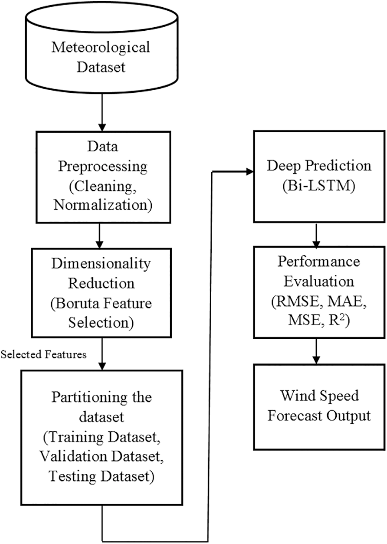
Figure 2: The proposed BFS-Bi-LSTM prediction model

Finally, it marks the importance of each original feature. When the z-score of the original feature is greater than the maximum z-score value of its all shadow features original feature is marked as important. Otherwise, it is marked as unimportant. Repeat the process until all features are marked or the predefined number of iterations is met. It creates the list of the important features from the original features and also forms the reduced dataset. Then, it partitions the dataset into training, validation and testing datasets. After that, it builds the Bi-LSTM model and compares its performance against MLP, LSTM, Bi-LSTM, BFS-MLP and BFS-LSTM in terms of error measures root mean square error (RMSE), mean absolute error (MAE), mean square error (MSE) and coefficient of determination (R2). As Bi-LSTM has its intrinsic feature extraction capability, the external Boruta feature selection helps to remove the non-informative and irrelevant features before the prediction process. Hence, it enables the model to perform accurate wind speed forecasting with optimal features. As the Bi-LSTM has its intrinsic feature extraction capability, the Boruta feature selection helps to reduce the complexity of the model greatly and guarantees an improvement in the accuracy of wind speed forecasting.

4  Performance Analysis

Generally, there are numerous ways to evaluate the prediction model performance. In this paper, the performance of the model is evaluated in terms of RMSE, MAE, MSE and coefficient of determination (R2). The RMSE is defined as the difference between forecast value and actual value [48,49]. It shows the square root of the variance of residuals. It is calculated at different time intervals as follows,

RMSE=1N∑t=1N(At−Ft)2 (7)

MAE is defined as the average of the absolute difference between prediction and actual observation over ‘N’ samples. It is calculated as follows,

MAE = 1N∑t=1N|At−Ft| (8)

MSE is defined as the mean of the squared difference between predicted and actual observation over ‘N’ samples. It is calculated as follows,

MSE = 1N∑t=1N(At−Ft)2 (9)

where ‘N’ represents the number of observations, ‘At’ represents the actual wind speed for the period ‘t’, ‘Ft’ represents the predicted wind speed for the period ‘t’. The R2 is called the coefficient of determination that helps to find the fitness of the model. It shows how well the predicted wind speed is similar to the actual wind speed. The value of R2 lies in the range of 0 to 1. It gets the value 1when the model closely fits with the actual value. Otherwise, it gets the value 0. The R2 is calculated as follows,

R2=1−∑(a^i−ai)2∑(ai−a¯i)2 (10)

where ‘ai’ represents the actual value, a^i represents the forecast value, a¯ represents the mean value.

5  Experimental Results and Discussion

The proposed BFS-Bi-LSTM model is experimented in a Tensorflow environment using the meteorological dataset of the European country. The dataset consists of meteorological data recorded in an hourly basis for the six years from January 2015 to November 2021. It includes the features of different meteorological characteristics such as Temperature, Radiation, Precipitation, Geopotential, Agriculture and Wind. The list of original features are F1-Date, F2-Wind speed, F3-Wind direction, F4-Temperature at 2 m elevation, F5- Growing Degree Days at 2 m elevation, F6-Temperature at 1000 mb, F7-Temperature at 850 mb, F8-Temperature at 700 mb, F9- Sunshine Duration, F10-Shortwave Radiation, F11-Direct Shortwave Radiation, F12-Diffuse Shortwave Radiation, F13-Precipitation Total, F14- Snowfall Amount, F15- Relative Humidity, F16-Cloud Cover Total, F17-Cloud Cover High, F18-Cloud Cover Medium, F19-Cloud Cover Low, F20- CAPE, F21-Mean Sea Level Pressure, F22-Geopotential Height at1000 mb, F23-Geopotential Height at 850 mb, F24-Geopotential Height at 700 mb, F25-Geopotential Height at 500 mb, F26-Evapotranspiration, F27- FAO Reference, F28-Surface Skin Temperature, F29-Soil Temperature, F30-Soil Moisture and F31-Vapor Pressure Deficit. It has 31 features and 60624 instances. The dataset is partitioned into 60:20:20 ratio instances for constructing training, validation and testing datasets. The meteorological data and wind speed are given as input for training the model and the wind speed for the future period is forecasted. The sample of actual wind speed is shown in Fig. 3.

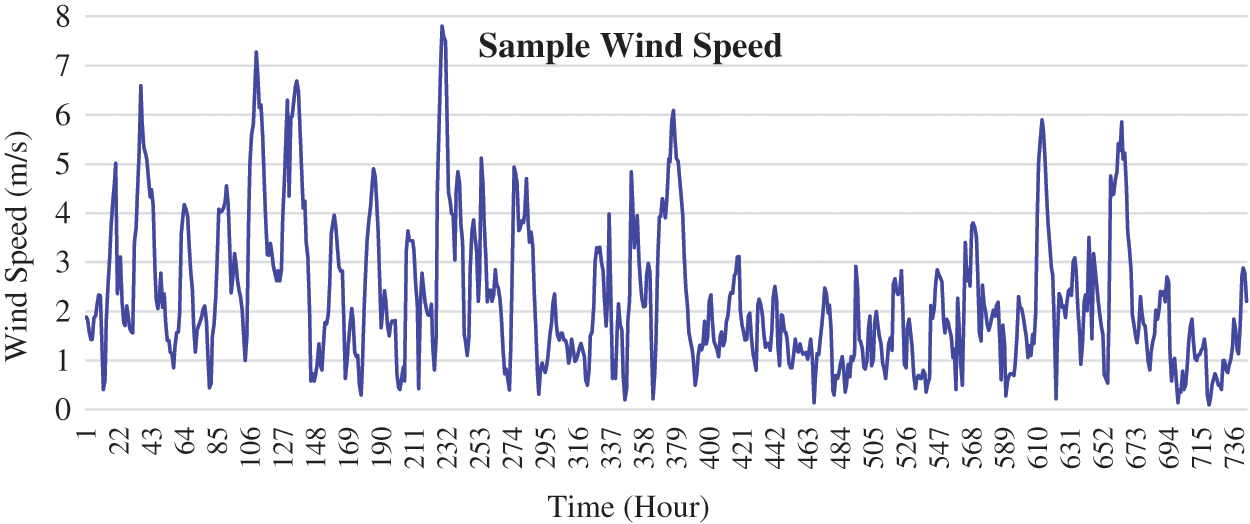
Figure 3: Example wind speed

The Boruta feature selection identified 13 features as the relevant features related to wind speed. They are F3, F4, F7, F8, F11, F15, F22, F26, F27, F28, F29, F30 and F31. The temperature, radiation, precipitation, agriculture and wind related features show their dominant relationship with the target wind speed. The dataset with these selected features is given as input for the deep prediction process. The Bi-LSTM network is configured as the three hidden layers of the network with 40 neurons in each layer. The number of neurons for each hidden layer is fixed by testing the Bi-LSTM network by varying the number of neurons from 10 to 70. Similarly, the number of epochs is fixed for the Bi-LSTM network by varying the epochs from 10 to 150. Finally, at the 110th iteration with 40 neurons in each layer achieve minimum mean absolute error. The MAE for the number of epochs and the number of neurons is shown in Fig. 4.

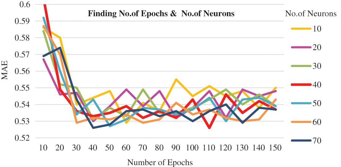
Figure 4: Number of epochs vs. number of neurons

The number of hidden layers is fixed as 3, the number of epochs is fixed as 110 and the number of neurons in each layer is fixed as 40. The optimizer used is Adam and the loss function used is mean absolute error. The Bi-LSTM network is trained, validated and tested using the training, validation and testing datasets. The wind speed is forecasted by building MLP, LSTM and Bi-LSTM models without feature selection and with feature selection. Fig. 5 shows a sample of actual and predicted wind speed using MLP, LSTM and Bi-LSTM. The graph is shown in Fig. 5i represents the wind speed predicted by MLP has much deviation in many timesteps with actual observed wind speed. The predicted wind speed of LSTM is shown in Fig. 5ii. It presents the forecast wind speed of LSTM is closer with the actual wind speed compared to MLP. The forecast wind speed of Bi-LSTM in Fig. 5iii is more closer to the actual wind speed than MLP and LSTM. Hence, it shows that the predicted wind speed of Bi-LSTM is almost closer to the actual wind speed compared to other models. It confirms that the Bi-LSTM outperforms other models. The forecasting models are tested by building them with selected features of Boruta. Fig. 6 shows a sample of actual and predicted wind speed using BFS-MLP, BFS-LSTM and BFS-Bi-LSTM. Fig. 6i presents the comparison of actual and forecast wind speed of BFS-MLP. It shows that MLP with Boruta feature selection produces better results compared to MLP. The graph in Fig. 6ii illustrates the forecast wind speed of LSTM with selected features provides better forecasting results than BFS-MLP. The forecast graph is closer to the actual wind speed graph. Fig. 6iii shows the forecast wind speed using Bi-LSTM with selected features graph almost closer to the actual wind speed graph compared to MLP, LSTM, BFS-MLP and BFS-LSTM. Figs. 5 and 6 show that the proposed BFS-Bi-LSTM surpassed other models by producing the forecast wind speed almost closer to the actual wind speed.

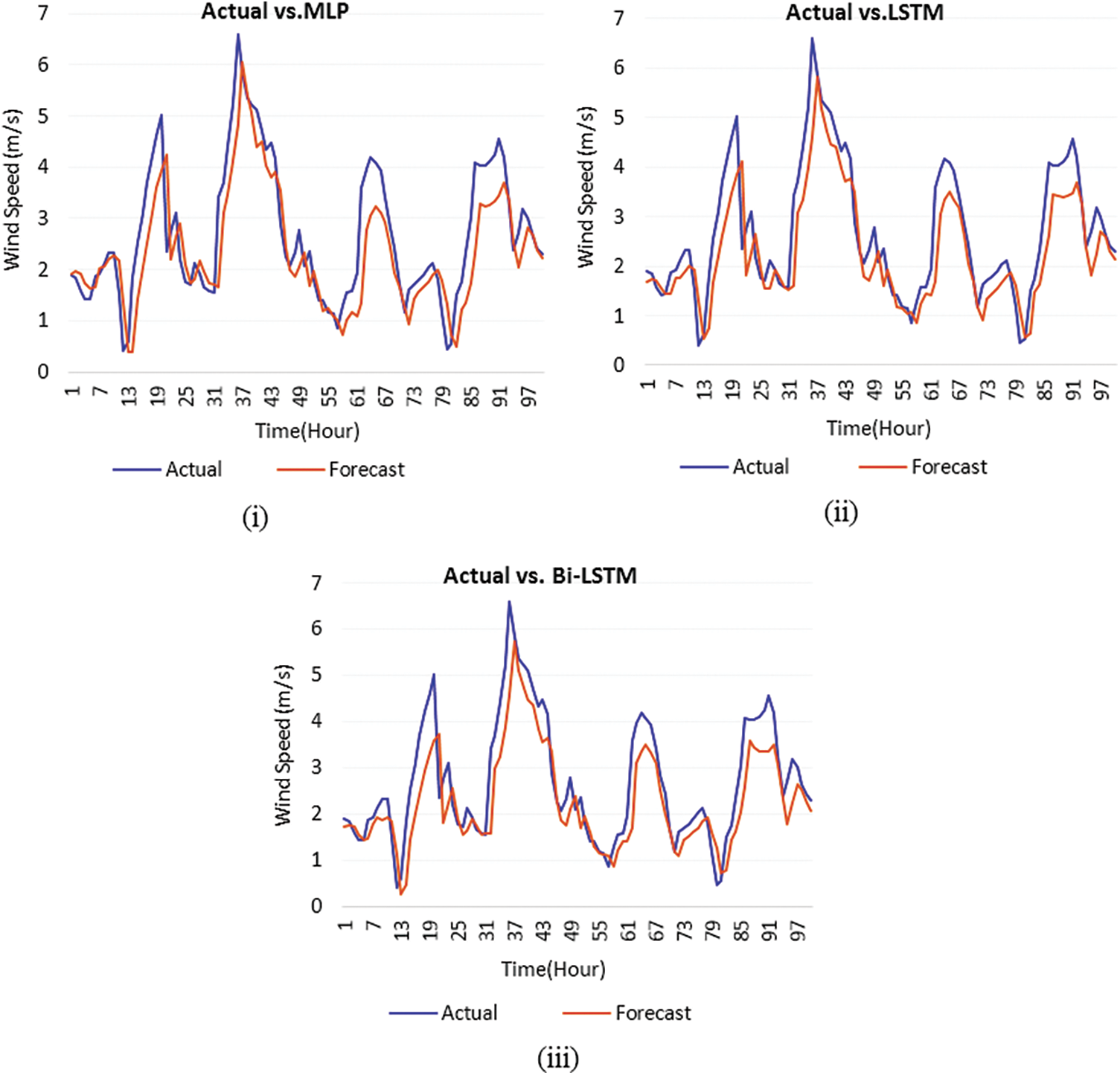
Figure 5: Comparison of forecast wind speed and actual wind speed (i) Actual vs. MLP (ii) Actual vs. LSTM (iii) Actual vs. Bi-LSTM

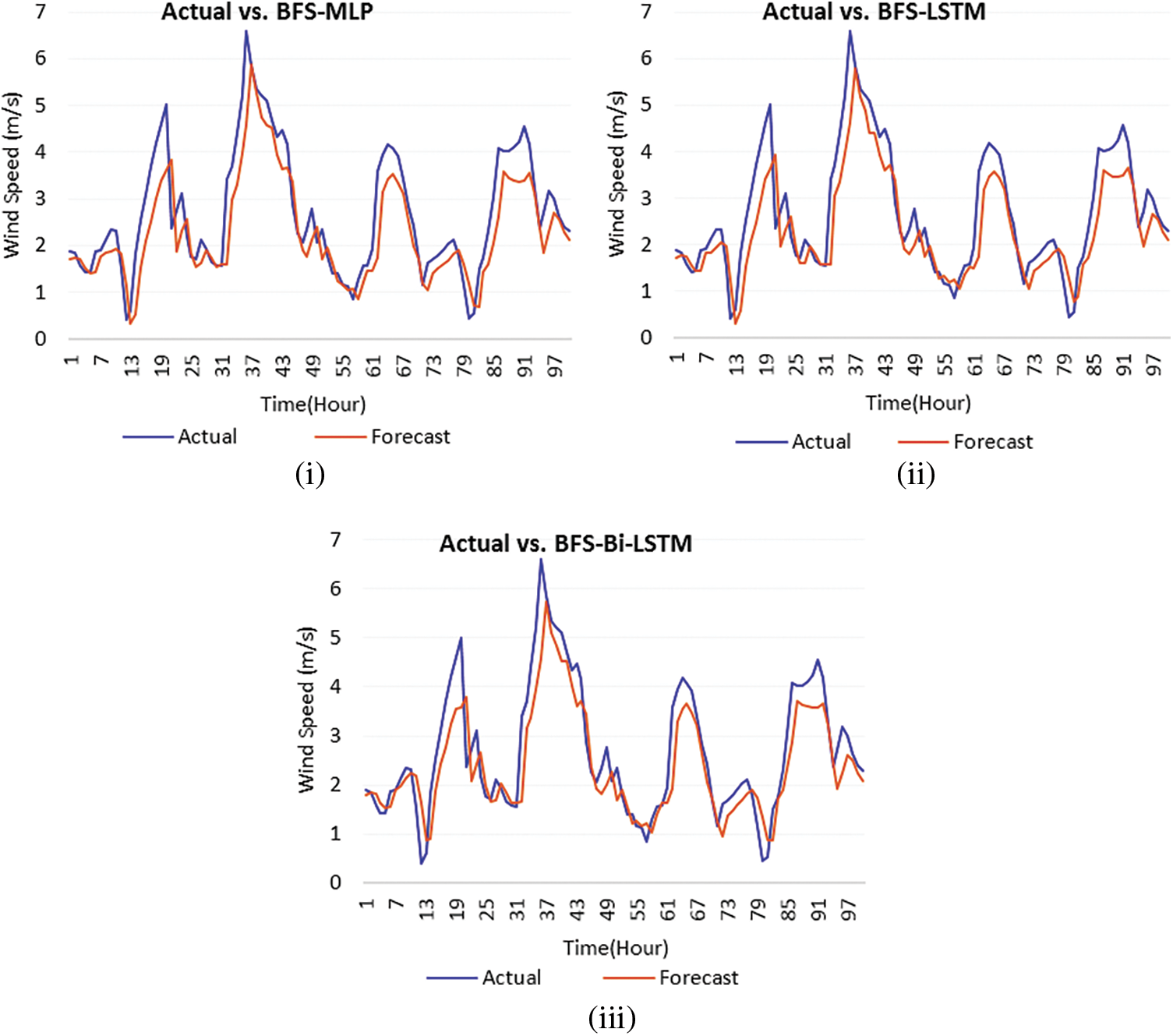
Figure 6: Comparison of forecast wind speed and actual wind speed (i) Actual vs. BFS-MLP (ii) Actual vs. BFS-LSTM (iii) Actual vs. BFS-Bi-LSTM

The comparison of forecast and actual wind speed using scatter plot is shown in Fig. 7. The correlation between actual and forecast wind speed shows how much the forecast wind speed is closer to an actual wind speed. The correlation value ranges from 0 to 1. When the correlation is 1, it represents the actual and forecast wind speed is same. When the correlation is 0, it represents the actual and forecast wind speed is different. Fig. 7a shows that the forecast wind speed of MLP has less similarity to the actual wind speed. It is denoted by the coefficient of determination R2 is 0.8684. Fig. 7b shows that the forecast wind speed of LSTM is better than MLP. The forecast wind speed of LSTM is more similar to the actual wind speed than MLP. The coefficient of determination R2 is 0.8765. Fig. 7c shows the similarity of Bi-LSTM forecasted wind speed is more with the actual wind speed than MLP and LSTM. The coefficient of determination R2 is 0.8718. Fig. 7d shows the forecast wind speed of MLP with selected features improves the forecasting result. The forecast wind speed is much closer to the actual wind speed compared to MLP, LSTM and Bi-LSTM. The coefficient of determination R2 is 0.8733. Fig. 7e shows the forecast wind speed of LSTM with selected features achieves a better forecast than MLP, LSTM, Bi-LSTM and BFS-MLP. The coefficient of determination R2 is 0.8737. Fig. 7f shows the forecast wind speed using Bi-LSTM with selected features (BFS-Bi-LSTM) is almost closer to the actual wind speed. The coefficient of determination R2 is 0.8766. BFS-Bi-LSTM outperforms MLP, LSTM, Bi-LSTM, BFS-MLP and BFS-LSTM.

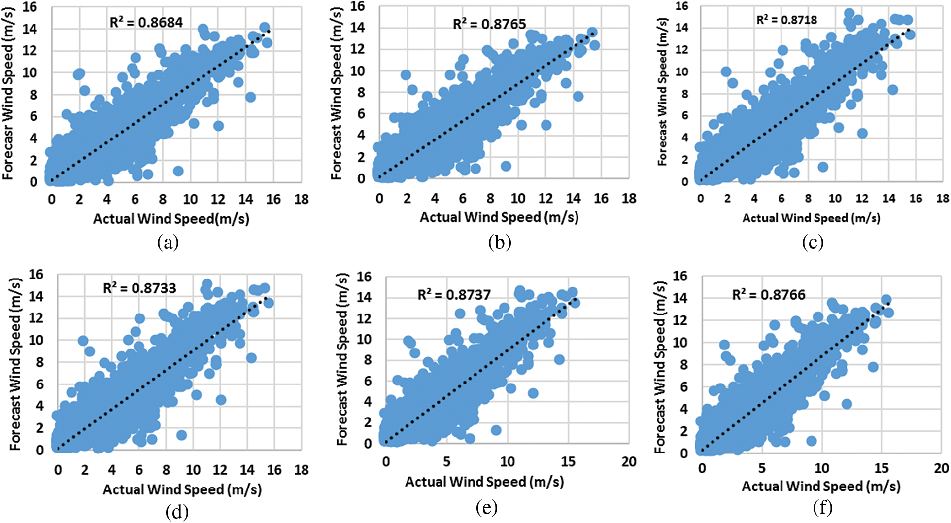
Figure 7: Scatterplot of actual and forecast wind speed (a) MLP (b) LSTM (c) Bi-LSTM (d) BFS-MLP (e) BFS-LSTM (f) BFS-Bi-LSTM

In this paper, the performance of forecasting models is evaluated using error measures such as RMSE, MAE, MSE and coefficient of determination R2. Tab. 1 shows the comparison of forecasting results using statistical measures and error measures.

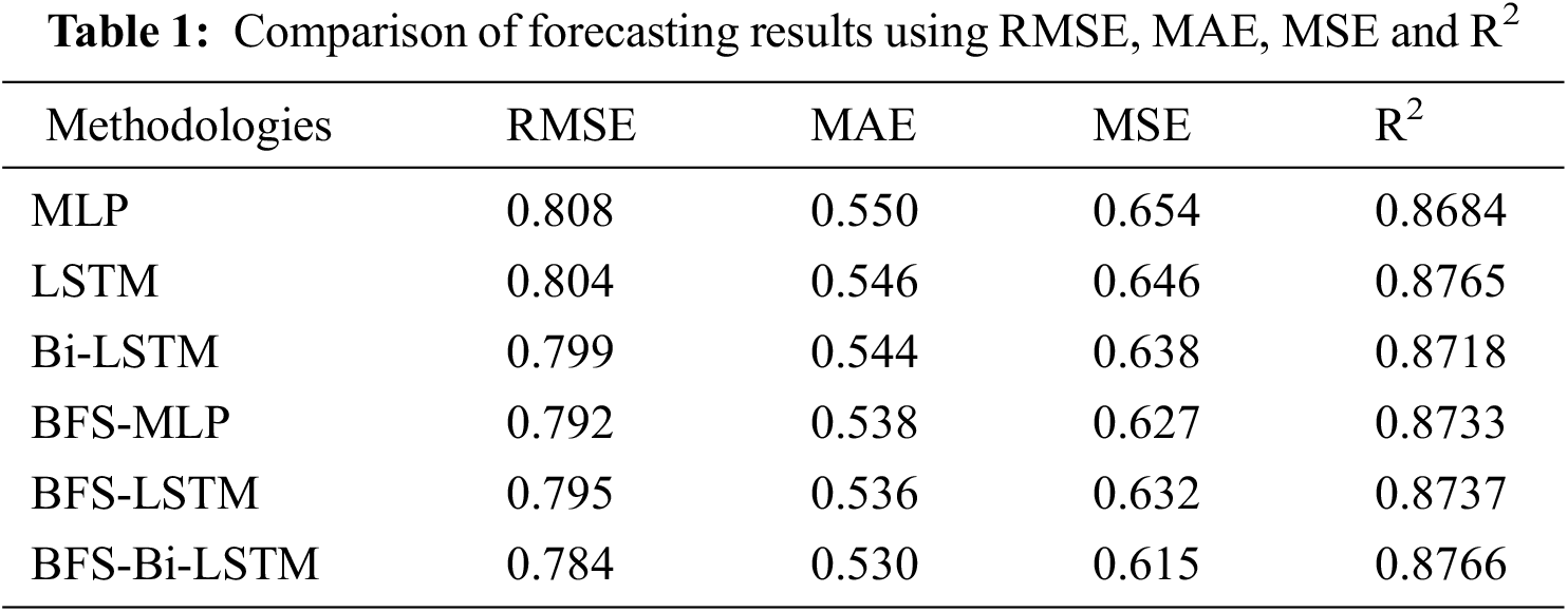
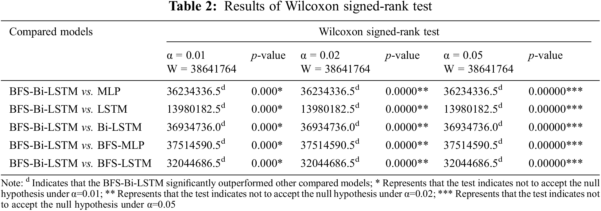
Tab. 1 shows the proposed BFS-Bi-LSTM surpassed other models by producing less root mean square error, mean absolute error and mean square error compared to MLP, LSTM, Bi-LSTM, BFS-MLP and BFS-LSTM. Similarly, it also confirms its superiority with other models by producing high R2 compared to MLP, LSTM, Bi-LSTM, BFS-MLP and BFS-LSTM. In addition to the error measures, the superiority of the proposed model is also proved by conducting the statistical test namely, Wilcoxon signed-rank test. It is a pairwise non-parametric test that is used to test the significance of one model against another model. It is utilized to compare the proposed model with each other competing model. In this paper, it is performed between two sets of the same size wind speed forecast data produced by two models. First, it assumes the hypothesis like the medians of the differences between two sets of data is the same. Then it calculates the Wilcoxon critical value as follows,

Wilcoxoncriticalvalue=Numberofdata(Numberofdata+1)4 (11)

After that, it calculates the Wilcoxon statistic value as follows,

Wilcoxonstatisticsvalue=minimum{r+,r−} (12)

where the ‘ r−’ denotes the sum of ranks of the second model is greater than the first model. The ‘r+’ denotes the sum of ranks of the second model is smaller than the first model. Finally, it compares the Wilcoxon statistic value with Wilcoxon critical value and rejects the hypothesis if the Wilcoxon statistic value is less than or equal to the Wilcoxon critical value [43]. The rejection of the hypothesis shows the improved performance of the proposed model. The results of the Wilcoxon signed-rank test is shown in Tab. 2.

6  Conclusion

Wind speed has a prominent role in wind energy forecasting. The forecasting of wind speed is indispensable for the accurate forecasting of wind energy. Nowadays harmless renewable energy generation is viable to secure the environment. In this paper, deep learning based wind speed forecasting using Bi-LSTM with Boruta wrapper feature selection was proposed. The model identified all the highly correlated meteorological features for wind speed using Boruta feature selection and performed the wind speed forecasting using Bi-LSTM. The fitting of the model was evaluated in terms of error measures such as RMSE, MAE, MSE and coefficient of determination R2. The proposed BFS-Bi-LSTM model is compared against MLP, LSTM, Bi-LSTM, BFS-MLP and BFS-LSTM. The result shows that the proposed BFS-Bi-LSTM surpassed other models by producing less mean absolute error, mean square error and root mean square error compared to MLP, LSTM, Bi-LSTM, BFS-MLP and BFS-LSTM. Similarly, it also confirms its superiority with other models by producing high R2 compared to MLP, LSTM, Bi-LSTM, BFS-MLP and BFS-LSTM. In future, the decomposition techniques, other deep learning methodologies, transfer learning concepts and attention mechanisms can also be utilized to improve the performance of the wind speed forecasting.

Funding Statement: The authors received no specific funding for this study.

Conflicts of Interest: The authors declare that they have no conflicts of interest to report regarding the present study

References

 1.  A. Ibrahim, S. Mirjalili, M. El-Said, S. S. Ghoneim, M. M. Al-Harthi et al., “Wind speed ensemble forecasting based on deep learning using adaptive dynamic optimization algorithm,” IEEE Access, vol. 9, pp. 125787–125804, 2021. [Google Scholar]

 2.  Z. Guo, W. Zhao, H. Lu and J. Wang, “Multi-step forecasting for wind speed using a modified EMD-based artificial neural network model,” Renewable Energy, vol. 37, no. 1, pp. 241–249, 2012. [Google Scholar]

 3.  L. Huang, L. Li, X. Wei and D. Zhang, “Short-term prediction of wind power based on BiLSTM–CNN–WGAN-GP,” Soft Computing, pp. 1–15, 2022. [Google Scholar]

 4.  S. Mehdizadeh, A. Kozekalani Sales and M. J. S. Safari, “Estimating the short-term and long-term wind speeds: Implementing hybrid models through coupling machine learning and linear time series models,” SN Applied Sciences, vol. 2, no. 6, pp. 1–15, 2020. [Google Scholar]

 5.  G. Alkhayat and R. Mehmood, “A review and taxonomy of wind and solar energy forecasting methods based on deep learning,” Energy and AI, vol. 4, pp. 100060, 2021. [Google Scholar]

 6.  U. Singh, M. Rizwan, M. Alaraj and I. Alsaidan, “A machine learning-based gradient boosting regression approach for wind power production forecasting: A step towards smart grid environments,” Energies, vol. 14, no. 16, pp. 5196, 2021. [Google Scholar]

 7.  M. Ali, A. Khan and N. U. Rehman, “Hybrid multiscale wind speed forecasting based on variational mode decomposition,” International Transactions on Electrical Energy Systems, vol. 28, no. 1, pp. e2466, 2018. [Google Scholar]

 8.  T. Wang, “A combined model for short-term wind speed forecasting based on empirical mode decomposition, feature selection, support vector regression and cross-validated lasso,” PeerJ Computer Science, vol. 7, pp. e732, 2021. [Google Scholar]

 9.  P. S. Kumar, “Improved prediction of wind speed using machine learning,” EAI Endorsed Trans Energy Web, vol. 6, no. 23, pp. 1–7, 2019. [Google Scholar]

10. J. Quan and L. Shang, “Short-term wind speed forecasting based on ensemble online sequential extreme learning machine and Bayesian optimization,” Mathematical Problems in Engineering, vol. 2020, pp. 1–13, 2020. [Google Scholar]

11. S. Salcedo-Sanz, L. Cornejo-Bueno, L. Prieto, D. Paredes and R. García-Herrera, “Feature selection in machine learning prediction systems for renewable energy applications,” Renewable and Sustainable Energy Reviews, vol. 90, pp. 728–741, 2018. [Google Scholar]

12. S. S. Subbiah and J. Chinnappan, “A review of bio-inspired computational intelligence algorithms in electricity load forecasting,” Smart Buildings Digitalization, vol. 1, pp. 169–192, 2022. [Google Scholar]

13. P. S. Kumar, “A review of soft computing techniques in short-term load forecasting,” International Journal of Applied Engineering Research, vol. 12, no. 18, pp. 7202–7206, 2017. [Google Scholar]

14. P. S. Kumar and D. Lopez, “Forecasting of wind speed using feature selection and neural networks,” International Journal of Renewable Energy Research, vol. 6, no. 3, pp. 833–837, 2016. [Google Scholar]

15. P. S. Kumar and D. Lopez, “Feature selection used for wind speed forecasting with data driven approaches,” Journal of Engineering Science and Technology Review, vol. 8, no. 5, pp. 124–127, 2015. [Google Scholar]

16. G. Swaroop, P. S. Kumar and T. M. Selvan, “An efficient model for share market prediction using data mining techniques,” International Journal of Applied Energy Research, vol. 9, no. 17, pp. 3807–3812, 2014. [Google Scholar]

17. H. Liu, X. Mi and Y. Li, “Smart deep learning based wind speed prediction model using wavelet packet decomposition, convolutional neural network and convolutional long short term memory network,” Energy Conversion and Management, vol. 166, pp. 120–131, 2018. [Google Scholar]

18. C. Zhang, H. Wei, J. Zhao, T. Liu, T. Zhu et al., “Short-term wind speed forecasting using empirical mode decomposition and feature selection,” Renewable Energy, vol. 96, pp. 727–737, 2016. [Google Scholar]

19. X. Liu, H. Zhang, X. Kong and K. Y. Lee, “Wind speed forecasting using deep neural network with feature selection,” Neurocomputing, vol. 397, pp. 393–403, 2020. [Google Scholar]

20. H. Liu, Z. Duan, H. Wu, Y. Li and S. Dong, “Wind speed forecasting models based on data decomposition, feature selection and group method of data handling network,” Measurement, vol. 148, pp. 106971, 2019. [Google Scholar]

21. L. Chen, Z. Li and Y. Zhang, “Multiperiod-ahead wind speed forecasting using deep neural architecture and ensemble learning,” Mathematical Problems in Engineering, vol. 2019, pp. 1–14, 2019. [Google Scholar]

22. A. Ghanbarzadeh, A. R. Noghrehabadi, M. A. Behrang and E. Assareh, “Wind speed prediction based on simple meteorological data using artificial neural network’”, in Proc. 7th Int. Conf. on Industrial Informatics, Cardiff, UK: IEEE, pp. 664–667, 2009. [Google Scholar]

23. M. Ibrahim, A. Alsheikh, Q. Al-Hindawi, S. Al-Dahidi and H. ElMoaqet, “Short-time wind speed forecast using artificial learning-based algorithms,” Computational Intelligence and Neuroscience, vol. 2020, pp. 1–15, 2020. [Google Scholar]

24. I. Marovic, I. Susanj and N. Ozanic, “Development of ANN model for wind speed prediction as a support for early warning system,” Complexity, vol. 2017, pp. 1–10, 2017. [Google Scholar]

25. C. J. Huang and P. H. Kuo, “A short-term wind speed forecasting model by using artificial neural networks with stochastic optimization for renewable energy systems,” Energies, vol. 11, no. 10, pp. 2777, 2018. [Google Scholar]

26. P. S. Kumar and D. Lopez, “A review on feature selection methods for high dimensional data,” International Journal of Engineering and Technology, vol. 8, no. 2, pp. 669–672, 2016. [Google Scholar]

27. V. G. Kiruthika, V. Arutchudar and P. S. Kumar, “Highest humidity prediction using data mining techniques,” International Journal of Applied Engineering Research, vol. 9, no. 16, pp. 3259–3264, 2014. [Google Scholar]

28. U. Sanusi and D. Corne, “Feature selection for accurate short-term forecasting of local wind-speed,” in 8th Int. Workshop on Computational Intelligence and Applications, Hiroshima, Japan: IEEE, pp. 121–126, 2015. [Google Scholar]

29. S. S. Subbiah and J. Chinnappan, “Short-term load forecasting using random forest with entropy-based feature selection,” in Artificial Intelligence and Technologies, Lecture Notes in Electrical Engineering, Singapore: Springer, vol. 806, 2022. [Google Scholar]

30. S. S. Subbiah and J. Chinnappan, “Opportunities and challenges of feature selection methods for high dimensional data: A review,” Ingénierie des Systèmes D’Information, vol. 26, no. 1, pp. 67–77, 2021. [Google Scholar]

31. C. Feng, M. Cui, B. M. Hodge and J. Zhang, “A data-driven multi-model methodology with deep feature selection for short-term wind forecasting,” Applied Energy, vol. 190, pp. 1245–1257, 2017. [Google Scholar]

32. G. Dong and H. Liu, Feature engineering for machine learning and data analytics, CRC Press, Boca Raton, FL, 2018. [Google Scholar]

33. M. B. Kursa and W. R. Rudnicki, “Feature selection with the boruta package,” Journal of Statistical Software, vol. 36, no. 11, pp. 1–13, 2010. [Google Scholar]

34. K. U. Jaseena and B. C. Kovoor, “Decomposition-based hybrid wind speed forecasting model using deep bidirectional LSTM networks,” Energy Conversion and Management, vol. 234, pp. 113944, 2021. [Google Scholar]

35. A. Karmel, M. Adhithiyan and P. S. Kumar, “Machine learning based approach for pothole detection,” International Journal of Civil Engineering and Technology, vol. 9, no. 5, pp. 882–888, 2018. [Google Scholar]

36. S. Sivasankari and T. Lakshmi, “Operational analysis of various text mining tools in bigdata,” International Journal of Pharmacy & Technology, vol. 8, no. 2, pp. 4087–4091, 2016. [Google Scholar]

37. N. Agila and P. S. Kumar, “An efficient crop identification using deep learning,” International Journal of Scientific & Technology Research, vol. 9, no. 1, pp. 2805–2808, 2020. [Google Scholar]

38. S. S. Subbiah and J. Chinnappan, “An improved short term load forecasting with ranker based feature selection technique,” Journal of Intelligent & Fuzzy Systems, vol. 39, no. 5, pp. 6783–6800, 2020. [Google Scholar]

39. S. S. Subbiah and J. Chinnappan, “A review of short term load forecasting using deep learning,” International Journal on Emerging Technologies, vol. 11, no. 2, pp. 378–384, 2020. [Google Scholar]

40. S. Harbola and V. Coors, “Deep learning model for wind forecasting: Classification analyses for temporal meteorological data,” PFG–Journal of Photogrammetry, Remote Sensing and Geoinformation Science, vol. 90, no. 2, pp. 21–22, 2022. [Google Scholar]

41. J. Xiang, Z. Qiu, Q. Hao and H. Cao, “Multi-time scale wind speed prediction based on WT-bi-LSTM,” in Proc. Int. Conf. on Computer Science Communication and Network Security, MATEC Web of Conf., Sanya, China, vol. 309, pp. 05011, 2020. [Google Scholar]

42. V. K. Saini, R. Kumar, A. Mathur and A. Saxena, “Short term forecasting based on hourly wind speed data using deep learning algorithms,” in Proc. 3rd Int. Conf. on Emerging Technologies in Computer Engineering: Machine Learning and Internet of Things (ICETCE), Jaipur, India: IEEE, pp. 1–6, 2020. [Google Scholar]

43. G. Memarzadeh and F. Keynia, “A new short-term wind speed forecasting method based on fine-tuned LSTM neural network and optimal input sets,” Energy Conversion and Management, vol. 213, pp. 112824, 2020. [Google Scholar]

44. W. H. Lin, P. Wang, K. M. Chao, H. C. Lin, Z. Y. Yang et al., “Wind power forecasting with deep learning networks: Time-series forecasting,” Applied Sciences, vol. 11, no. 21, pp. 10335, 2021. [Google Scholar]

45. H. Liu, C. Chen, X. Lv, X. Wu and M. Liu, “Deterministic wind energy forecasting: A review of intelligent predictors and auxiliary methods,” Energy Conversion and Management, vol. 195, pp. 328–345, 2019. [Google Scholar]

46. S. K. Paramasivan, “Deep learning based recurrent neural networks to enhance the performance of wind energy forecasting: A review,” Revue D’Intelligence Artificielle, vol. 35, no. 1, pp. 1–10, 2021. [Google Scholar]

47. K. U. Jaseena and B. C. Kovoor, “A hybrid wind speed forecasting model using stacked autoencoder and LSTM,” Journal of Renewable and Sustainable Energy, vol. 12, no. 2, pp. 023302, 2020. [Google Scholar]

48. S. S. Subbiah and P. S. Kumar, “Deep learning based load forecasting with decomposition and feature selection techniques,” Journal of Scientific & Industrial Research, vol. 81, no. 5, pp. 505–517, 2022. [Google Scholar]

49. S. S. Subbiah and J. Chinnappan, “Deep learning based short term load forecasting with hybrid feature selection,” Electric Power Systems Research, vol. 210, pp. 108065, 2022. [Google Scholar]