Temporal Preferences-Based Utility Control for Smart Homes

1  Introduction

The Average to Peak (A2P) ratio is one of the most important parameters for managing an efficient and cost-effective power system. A high A2P ratio indicates peaks and troughs in demand, forcing energy managers to invest in expensive peak power plants that operate in the short term. In building management systems based on renewable energy, this results in a high initial cost of providing maximum energy. This is achieved by using more solar (photovoltaic or PV)/wind generators or more storage capacity. Various studies have highlighted this phenomenon [1–3]. Considering all A2P ratios, these ratios can increase up-front costs by a factor of 2.5 compared to the 65% case. Demand response is one of the most effective ways to reduce the A2P ratio, and much work remains to be done to reduce the capital cost of the system through smart device design. However, to the best of our knowledge, most studies focus on three aspects. In [1–3], the authors focus on providing price signals and financial incentives for home energy management to reduce A2P ratios. In [4–6], we can find a model user-friendly and control the process accordingly, reducing the A2P ratio as a by-product. In [7–10], the authors collect consumer preferences to reduce energy load, consumer input, comfort modeling and preference collection are more suitable for smart home and automation. If we examine these two modeling approaches in more detail, we see that comfort modeling is often limited to space heating and cooling. However, the authors did not observe any extension to other devices.

On the other hand, as far as the authors know, preference collection is usually static, as consumers are asked to choose a specific preference number, color, or level, and the algorithm then respects the same preference throughout their lifetime. This is the only viable solution, as regular likes can lead to consumer fatigue. Therefore, comfort modeling is a more ideal approach when possible. Extending comfort modeling to other devices essentially requires a way to compare the demands of using one device with another. Furthermore, comparison methods must take into account the temporal nature of preferences. If the room is consistently within 1 degree of the set point, the room must not be accepted, causing the contents of the refrigerator to rot. A better solution is to compare the importance or benefits of powering refrigerators, water pumps, and heating, ventilation, and air conditioning (HVAC) when demand is in short supply. To address this issue, in this paper we propose a new time-based utility method that opportunistically maximizes the use of available electricity to balance future demand by assigning a utility value to the usage of each controlled device. The utility assigns devices based on the level of service the device is currently providing to consumers. For example, if the room temperature is at the set point, the benefit is zero. If the room temperature deviates, the benefits grow exponentially based on past user experience. Likewise, utility values are assigned to each device based on the importance of the demand. This is quite different from the set of algorithms that require consumers to assign fixed priorities or importance to their devices [11,12] and systems that attempt to create user comfort profiles for individual devices for optimal planning [13–15]. The main contributions of this paper are as follows:

•   We proposed a Time Utility Based Control Feature (TUBCF) algorithm that automatically selects which devices to turn on and off based on the usefulness of the smart home.

•   We tested our algorithm on data from six households and minimized user inconvenience during peak hours. The Central Processing Unit (CPU) scheduling is implemented based on aging to prioritize different devices based on their usage.

•   We compare our results with the state-of-the-art Colored Power Algorithm (CPA), our Time-Based Utility Control Algorithm (TBUCA) algorithm that performs well during peak hours.

The rest of this work is planned as follows. In Section 2, we review related work. In Section 3, we present the system overview, discomfort parameters, and system model. In Section 4, we discuss a comparative analysis of the proposed system and discuss the results related to the CPU scheduling of the operating system. In the last section, we draw conclusions and future work.

2  Related Works

Optimal energy management at the household level has been extensively studied in the literature on the topic of on-demand response. From a design optimization perspective, we can classify work into three categories: financial incentives, comfort modeling, and user-defined priorities. In this section, we discuss work in these three areas separately. In [9], the authors propose an “Energy Planning System” to help consumers reduce their energy bills by knowing their equipment usage plans. The Enerplan system forms consumer categories based on regional statistics. This data can be used to determine device utilization and delivery to brand consumers. Based on this data, a device usage plan is created. Expert-based and automatically generated rules are used to generate usage plans. An efficient algorithm is proposed in [10]. The main goal of the algorithm is to reduce the peak-to-average ratio by operating selective devices when the grid is lightly loaded. All residential loads are divided into movable and immovable loads. To achieve the optimization of the load profile, load shifting and peak shaving techniques have been proposed. In [11], the authors propose a solution for efficient power consumption using Demand Side Management (DSM) for residential customers in Dhaka city. In their proposed strategy, three DSM tools of energy efficiency, direct control and time-sharing are used, and it is safe to use energy efficiency in large quantities.

In [12], an optimal planning procedure is planned for a series of household appliances under variable day-ahead peak prices. The main goal of this approach is to manage and schedule residential electricity demand under a dynamic pricing system, thereby reducing customers’ electricity bills. This problem has been outlined as the “multiple knapsack problem”, a well-known problem in computer science, which provides a cheap and efficient solution to the planning problem. The purpose of MKP is to distribute items in backpacks such that the total weight of each backpack is less than its capacity limit and the overall value within the backpack is maximized. In [13], an optimization model was developed using distributed power sources and batteries to handle the daily load of a single user and multiple users. The goal of their proposed solution is to minimize electricity bills and increase the efficiency of the grid. In [14], the authors of this paper anticipate a hybrid approach that combines Real-Time Price (RTP) and Inclined Block Rate (IBR). The goal of their research is to reduce electricity costs and PAR. The author divides home appliances into two categories: automatic home appliances and manual home appliances. The optimal electricity consumption planning method for all household based on RTP combined with IBR pricing scheme is proposed. RTP has more flexibility than TOU and key peak price. So the authors combine RTP and IBR, where the energy price for each time period varies according to the total electricity consumption.

In [15], the authors of this paper propose a reward-based algorithm for private clients. The purpose is to save network peaks. The proposed solution depends on the user’s preference, and the user is willing to participate in it for some reward. In [16] the authors proposed a new multi-objective algorithm for home appliances. The scheduling of appliances depends on the priority of real-time energy demand. The aim of this work is to improve energy planning for household consumer devices according to their operational priorities. In this work, they propose an Elitegroup Computer System (ECS) including planners and predictors installed in each home. Each ECS is connected to its neighbors through a Local Area Network (LAN). The purpose of this connection is to exchange intelligent information about sensors and energy consumption. In [17], the performance of a single family home is calculated by implementing a mixture of two techniques, namely Elephant Herding Optimization (EHO) and Enhanced Differential Evolution (EDE). The goal of this document is to minimize power costs and PAR while minimizing inconvenience to the user. RTP is used to calculate the cost of electricity.

3  Proposed System

There are many techniques in the literature for optimization and scheduling problems. In this study, two algorithms were used to compare power analysis, TBUCA and Color Power Algorithm (CPA). Although CPA effectively optimizes power consumption, its fixed-priority nature can increase user discomfort during peak hours. The purpose of our proposed TUBCF is to minimize user discomfort, which is the most fundamental challenge of Smart Grid (SG). We implemented both techniques on Pakistani household data for 7 days and showed that our proposed solution works well compared to CPA as it increases user discomfort due to its fixed priority nature. For user convenience, three parameters are defined including acceptable parameters, comfortable parameters and uncomfortable parameters. TUBCF is based on a utility function that reaches a magnitude that reflects the preferences of decision makers. Example: If U (AC) = 24 U (refrigerator) = 19, then AC is definitely better than a refrigerator. However, an air conditioner is not necessarily five times better than a refrigerator.

The word utility means order or hierarchy. So we use this concept to rank or rank the temporal preferences of devices that meet the user’s needs. In the utility function, we check the utility of the device against the current state of the device and the demand response form. Fig. 1 shows our proposed system model. We look at six smart home models that come with three devices, namely a water pump, an air conditioner, and a refrigerator. The utility script receives time-based consumption data from various smart devices of the smart home via Internet-of-Things (IoT)-based devices. The utility script then uses the utility function to find the utility for each home appliance. The result is passed to the controller. Depending on the usefulness of the device, the controller will turn the device on or off. In the below diagram, we can see that in the first 15 min decision, the refrigerator device is turned on, and in the next 15 min decision, the water pump is turned on and in the next 15 min, Air Conditioner is turned on depending upon their utility. In the following section, we discuss CPA and TUBCF in detail.

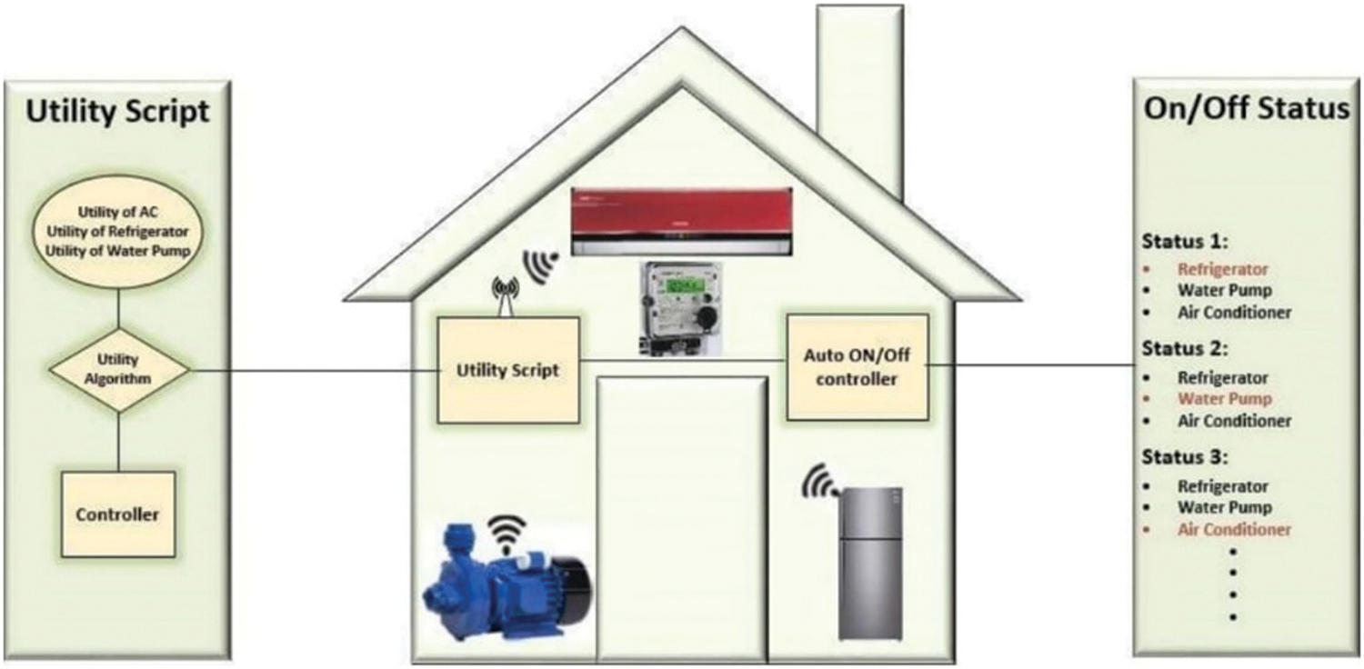
Figure 1: Proposed system model

3.1 Colored Power Algorithm

In [18], a Proto/Amorphous Cooperative Energy Management (PACEM) system for small cooperative residential users is proposed. The system is designed to address the challenges of consumer demand design through a simple qualitative interface for distributed control. In PACEM systems, the CPA has been proposed to reduce power consumption and thus manage demand shaping efficiently, but due to its fixed-priority nature, it increases user discomfort during peak periods. The functional plan is designed according to such colors. Fig. 2 shows the different color schemes. If the device is black, it will not be shut down at any time, red means it can only be shut down in an emergency, yellow means it can only be shut down at peak performance, green means it can be shut down or turned on at any time.

Figure 2: Overview of CPA system

Customers can participate in the system by assigning colors to their home appliances. The gateway device represents the home’s local demand management network, and the participating devices communicate with each other and with the gateway device. Feature plans are designed according to color with fixed priorities. If the device is black, it cannot be turned off at any time, red means it can only be turned off in an emergency, yellow means it can only be turned off at peak performance, and green means it can be turned off or turned on at any time. The technology has fixed priorities, so it cannot meet demand for certain devices, and targets a condition called “starvation”. Fig. 3 shows the Graphical User Interface (GUI) of CPA. The 6 houses show the implementation of CPA and users can assign different colors to the equipment according to their needs. We can see houses 2, 3, 4, 5 and 6, the device with the yellow icon is turned off during peak hours, even though the user needs it to function poorly, increasing consumer discomfort.

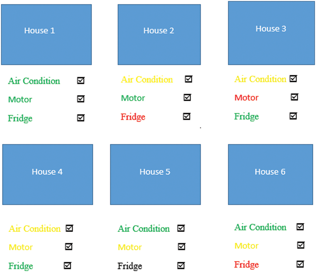
Figure 3: Graphical user interface of CPA system

3.2 Time Based Utility Control Function

Rather than fixing priorities or costing, we determine the value of equipment usage and allocate energy to the most needed equipment in descending order. We perform burn-in that produces a device time effect. In our proposed method, Time Based Utility Control Function (TUBCF), we find the consumption pattern of each device every 15 min, and then use the utility function to calculate the utility of each device. Turn on devices with high utility according to time preference.

Three main household appliances including AC, refrigerator, and water pump were used for experimental purposes. In the next section, a detailed description of our device and its implementation will be discussed. Eq. (1) represents the total utility of the device as follows,

While(allocated<supply)Allocated+={Load(i)|max[util(i))]}⇒∀i∈unallocated (1)

Fig. 4 shows the GUI of our proposed solution, which checks device availability every 15 min and decides to charge all devices based on our proposed mathematical model. When the supply is low, the device with the highest priority will be assigned according to the temporal preference in the assignment.

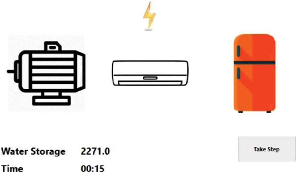
Figure 4: Graphical user interface of the proposed system

3.3 Experimental Setup

In our experimental phase, we had 6 houses with multiple appliances, but we only selected three appliances: water pump, air conditioner, and refrigerator. Let’s assume we have enough inventories to run one device at a time. Fig. 5 shows the constant power supply equal to 100 watts and the requirements for various devices. Refrigerator demand is greater than air conditioner and water pump. So the fridge suddenly asks for a cap.

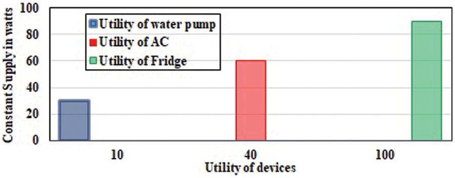
Figure 5: Supply and demand of different devices

3.3.1 Acceptable and Comfortable Parameters

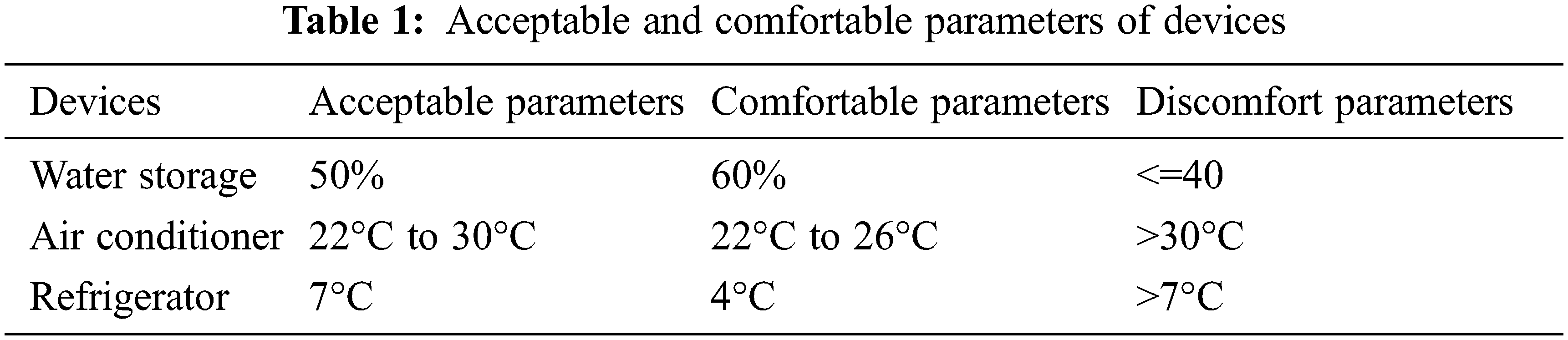
The main purpose of this study is to minimize user inconvenience, so in this section we will define the comfort and acceptable parameters for our three different devices: water motor, air conditioner and refrigerator. According to [19], a comfort zone is the situation, place or temperature in which you feel relaxed. The term acceptable level refers to conditions that are allowed or tolerated. For all equipment, we follow various comfort standards. A decision is underway on trends in vehicle water use. Refrigerator selection is based on the air conditioner’s decision on the target room temperature and compressor operating status. By replicating these patterns, we define acceptable and comfortable water storage parameters. With AC, the temperature of the room can be varied, which means comfortable housing.

The authors of [20] and [21] discuss the ideal comfort and acceptable room temperature for people in summer. Diet is an important part of our lives that allows us to have the energy to complete our daily tasks. In order to store food in the refrigerator, we need to know the correct temperature at which the food can be stored. According to the U.S. Food and Drug Administration (FDA) [22] guidelines for a temperature of 41°F to 135°F, stored food should be in a hazardous area. The United States Department of Agriculture (USDA) [23] defines this danger zone temperature as 40°F to 140°F. After a power outage, food will stay safe if the refrigerator temperature remains below 5°C (41°F). However, it is difficult to keep the temperature below 41°F when the unit is turned off. According to [24], at 10°C, stored food spoils much faster than at 5°C. The temperature danger zone describes the temperature range where bacteria grow faster, so try to keep your food out of the danger zone. Keep refrigerator temperature at or below 40°F per [22]. According to [23], the acceptable temperature for food is 7°C. See Tab. 1 for acceptable, comfort and discomfort parameters for different devices.

3.3.2 Water Pump

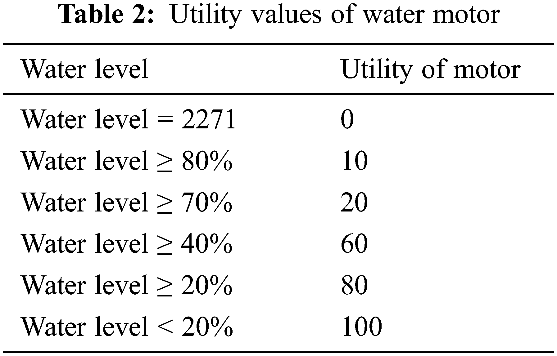
In our running example, our house has a water pump, which depends on the water consumption of a storage tank with a capacity of 2271 liters (600 gallons). To find the benefit of the water pump, we used the step function on this device. However, since the pedometer function has a constant value in certain intervals, the constant is different for each interval. In our case, the benefit is proportional to the water “use ∝ water level”. We compared the computational utility of each device. When the utility of the water pump is greater or higher than that of other equipment, start the engine. Tab. 2 shows the utility of the hydroelectric machine calculated using the step function.

3.3.3 Air Conditioner

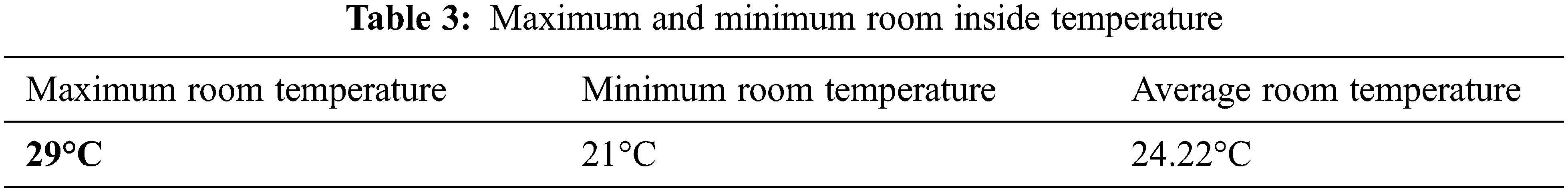
Air conditioning is a method of eliminating moisture and heat from the interior space of a living room to improve tenant comfort. To calculate the utility of alternating current, we use environmental variables such as indoor temperature and outdoor temperature. Eq. (2) represents the benefits of the Air Conditioner (AC), where “T” represents the temperature of the AC and the room temperature T inside, as follows,

AC(T)=eT(inside)1.72−14 (2)

We can use Eq. (2) to calculate the maximum and minimum room temperature. Tab. 3 gives the average to maximum and minimum temperatures.

3.3.4 Refrigerator

According to [24], refrigerators are the second largest electricity consumption (13.7%) after air conditioners (14.1%). Depending on their size, refrigerators use 100 to 400 watts, and large refrigerators use about 180 watts or 1575 kWh per year. These electricity rates do not depend on size, user behavior or occupancy [25]. Different electricity rates and refrigerator sizes are shown. In [26], the authors show that cooking activities, weekdays, weekends, and fasting also affect refrigerator energy consumption. When the refrigerator is placed in the kitchen and the oven is turned on for cooking, the room temperature will rise, which will affect the temperature of the refrigerator. The heating system must turn on the compressor to stabilize the internal temperature of the refrigerator. The energy consumption of a refrigerator depends on several variables as described in [26],

•   Number of doors opening

•   Duration of each door opening decision

•   Door opening speed

•   Ambient temperature

•   Thermostat setting position In this study, we consider these variables

•   Number of the door opening

•   Duration of the each door open

•   Thermostat setting position

•   How much heat is transferred each time when the door is open?

•   How much compressor time is required to run for a stable temperature?

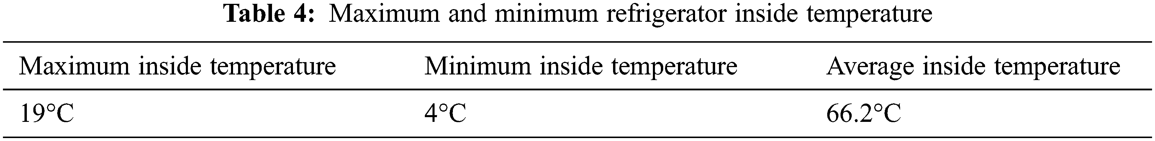
In [27], if the door of the refrigerator is not opened, the power is simply turned off and the refrigerator can only store cold food for 4 h. We only consider the door open decision, which is the main factor in increasing the compressor cycle. We open the refrigerator an average of 33 times a day. To find out how much heat is transferred every time the refrigerator door is opened, let’s do an experiment. In our experiments, we used a standard refrigerator with the refrigerator temperature set to 9°C and a meter with a sensor. We placed sensors inside the refrigerator and recorded its internal temperature at various intervals and each time the door was opened. Tab. 3 shows our results, in our experiments we found that the normal compressor cycle (turning hot to cold) is 5 min.

The compressor run time without opening the door depends on the thermocouple setting and the internal temperature. If the door is open for 5 min, the compressor cycle will increase from 5 to 7 min. We run this experiment every time the compressor cycles on and off. We put a sensor in the refrigerator when the compressor is on and get the internal temperature at different times. Tab. 4 shows the minimum, maximum and average internal temperatures of our refrigerators.

We can conclude that more doors open, more heat transfer and more compressors run time cycle and consume more electricity. The only reason the thermocouple turns on the compressor is for heat transfer. This can be caused by opening doors or placing food. But our focus is on opening the door. Eq. (3) represents the utility of the refrigerator as follows,

Fridge(T)={eTt(inside)2.61−4⇒ifT(inside)>60⇒Othersise (3)

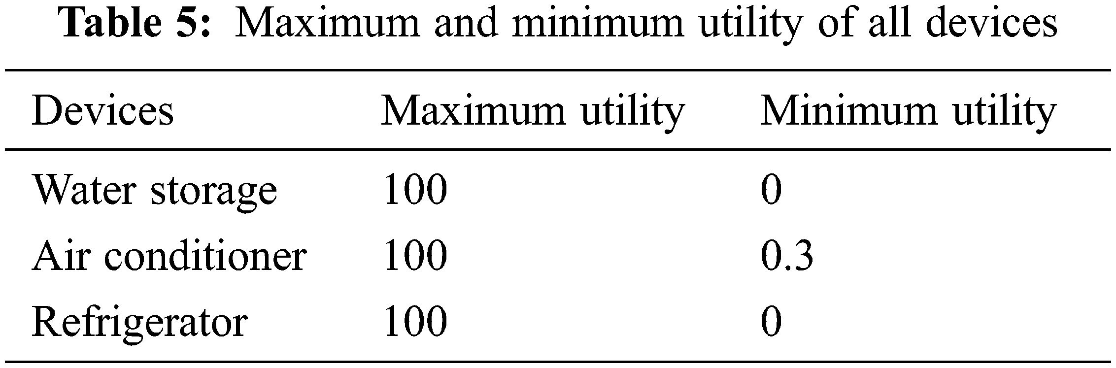
Tab. 5 shows our maximum and minimum utilities of all devices after performing the calculation.

4  Results and Discussion

To our knowledge, no other researchers have considered time-based preferences for these devices. State-of-the-art algorithms have fixed priorities, so starvation occurs. In this section, we compare fixed-priority CPAs by assigning four different colors (green, yellow, red, and black) to devices that perform time-based aging and TUBCF. We implemented both techniques on Pakistani household data and compared the results from 19:00 to 23:00, the peak time in Pakistan from June to August. The results show that our proposed solution performs well compared to color performance algorithms due to the increased user discomfort due to fixed priorities. Our proposed solution minimizes user discomfort in a better way. Consider house number 6, where the user has designated the water motor as yellow (off during peak hours). Fig. 6 shows the results of CPA, where 0 means off state, 1 means engine on state, the user wants to turn on the water pump, but since yellow is assigned, the engine needs to be turned off during peak periods, increasing the user’s discomfort.

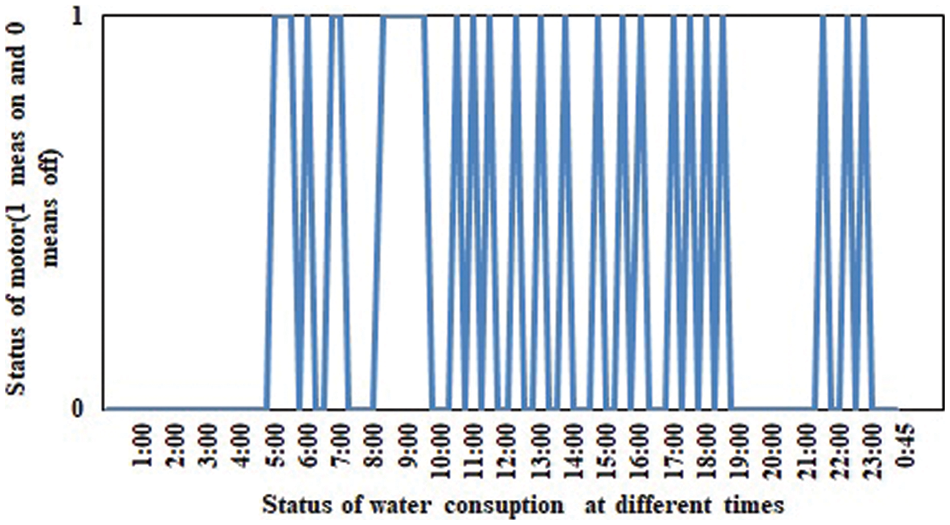
Figure 6: Motor status in peak hours

The results of our proposed solution TUBCF are shown in Fig. 7. Our utility script receives the consumption pattern of each device every 15 min and determines the usefulness of the device. Devices with high time priority are turned on. To calculate utility, we used Pakistani household data from three different devices in six different households. The utility of each device from six households is calculated every 15 min. Each device has a minimum or maximum number of benefits. In Fig. 7, the green line represents the water motor, and the motor state is on because it has the highest priority to the user in terms of time. We can see that although it is the peak time of Pakistan at 19:00 (19:00–22:00), the engine will be turned on according to the user’s time preference at that time, and it will be determined every 15 min to meet the needs of consumers during peak hours. Stop procrastinating, instead of permanently shutting down equipment during peak hours like with CPA.

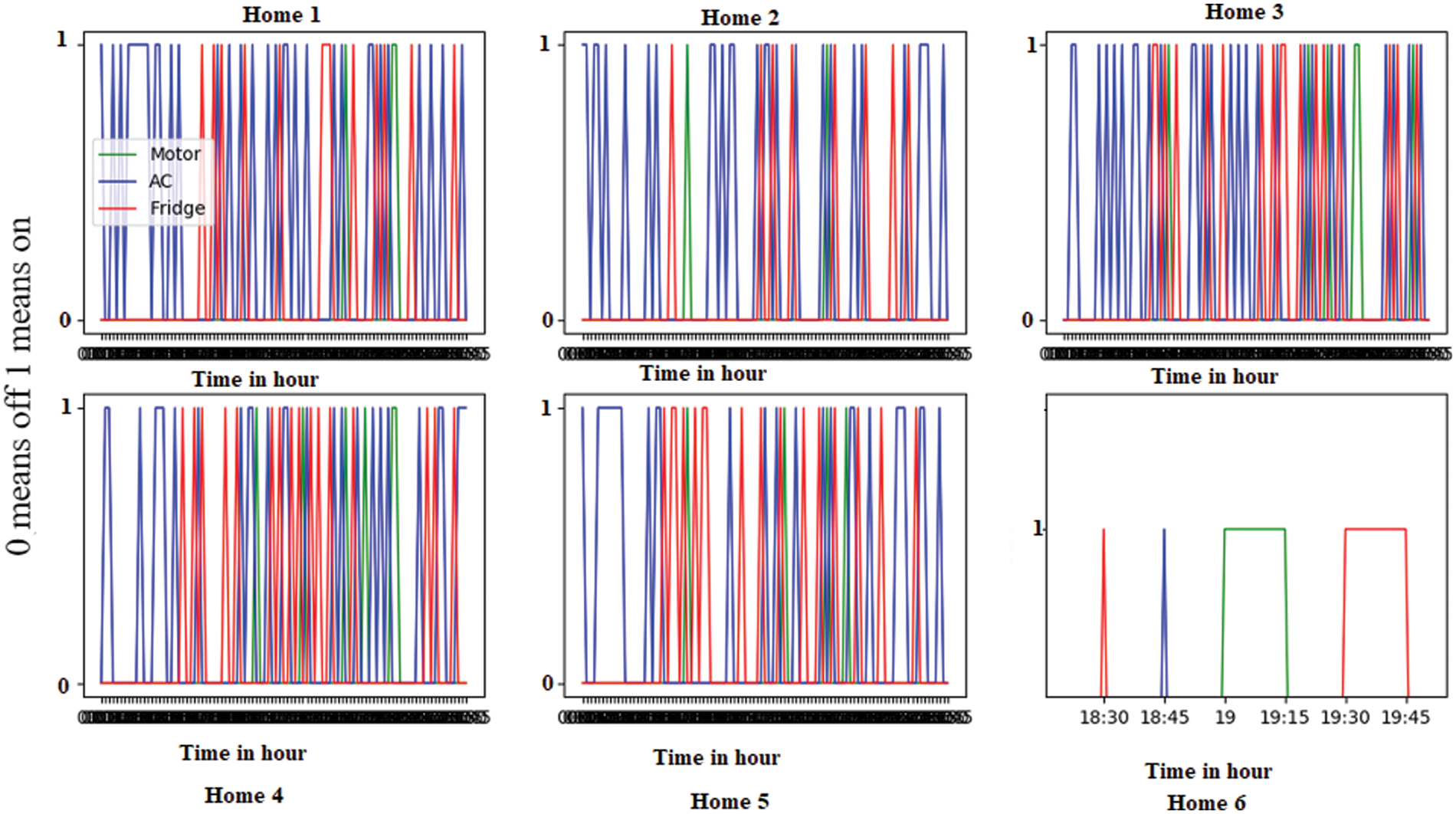
Figure 7: Result of TUBCF algorithm

4.1 Houses Implementation

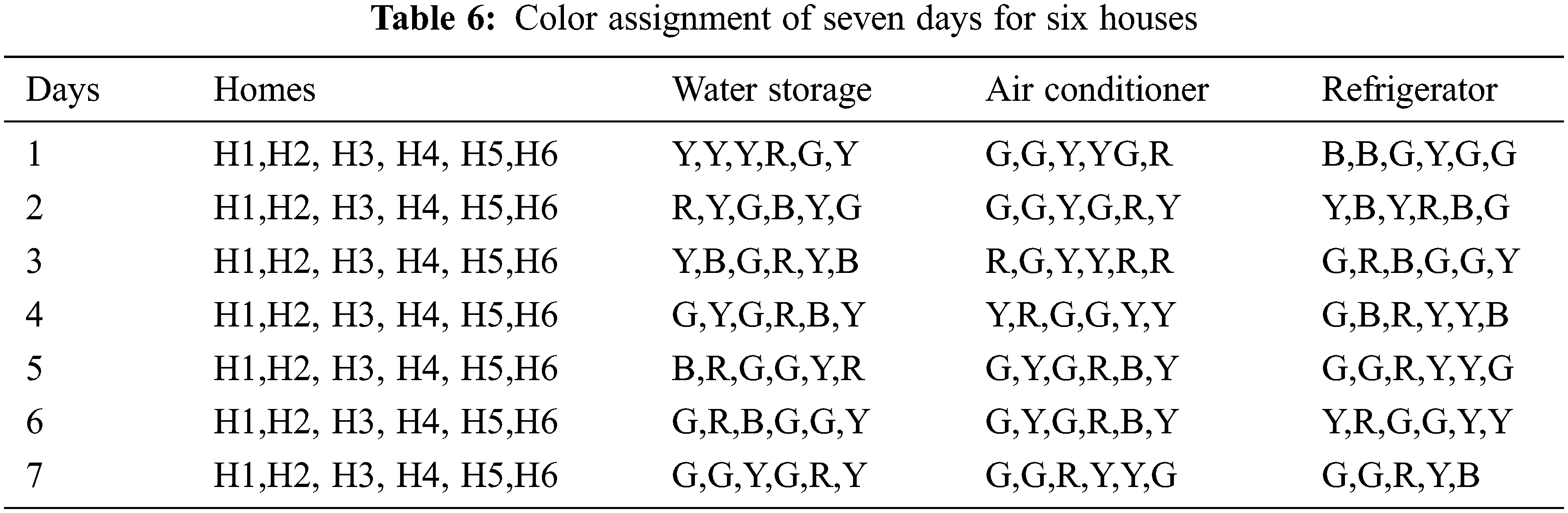
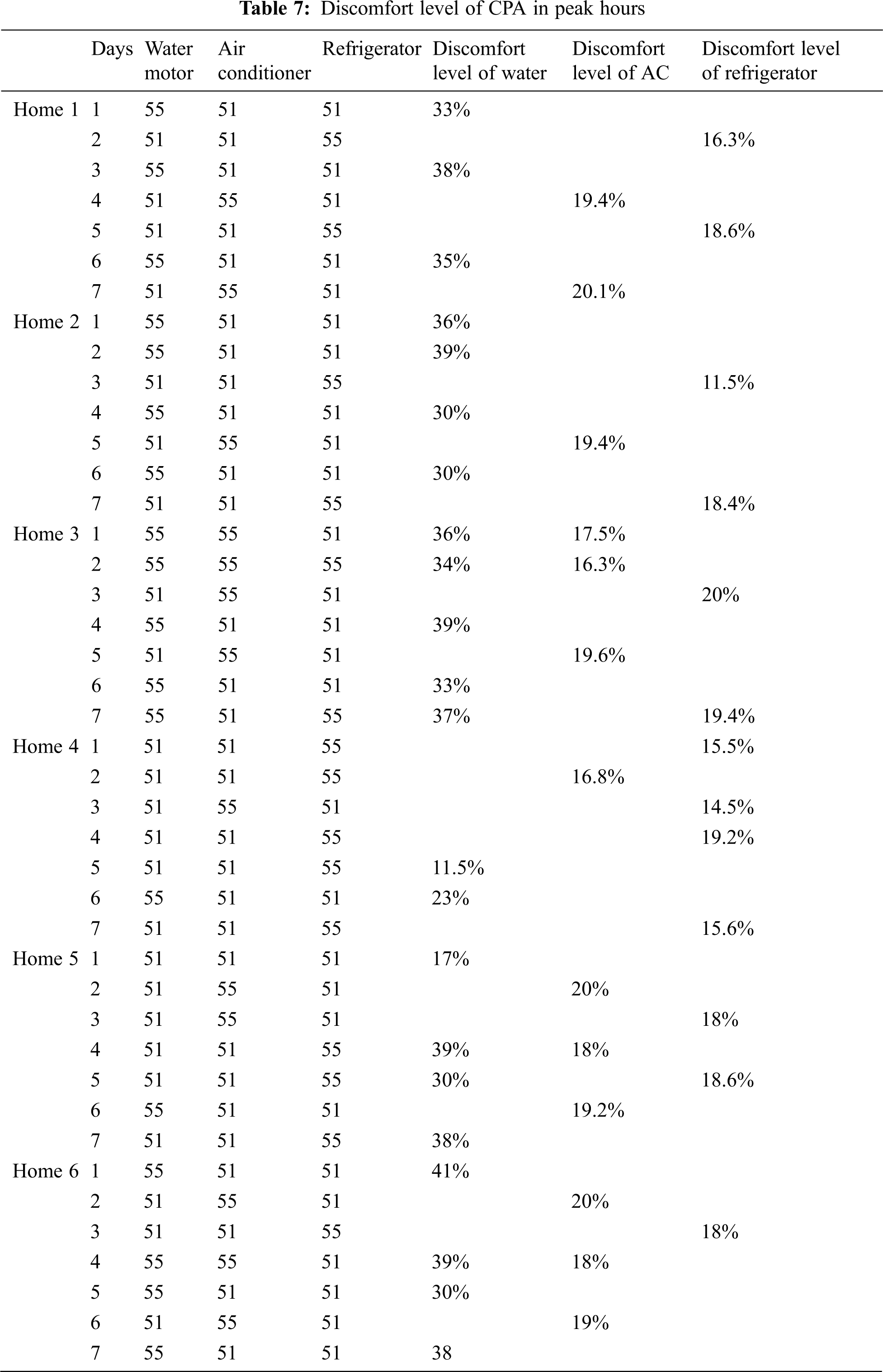
The CPA and TUBCF were implemented for 7 days on six households using the same equipment. The CPA assigned different devices to different colors for 7 days and found the discomfort level of each household after 15 min. For TUBCF, discomfort is calculated based on benefits. Tab. 6 shows the CPA implementation for 1 week for 6 houses, with 4 colors assigned to different devices. Yellow is (y) if the unit is yellow, it can only be closed during peak hours, green is (G) if the unit is green, it can be turned on and off at any time, red is (R) it can be in an emergency, black as (B) highlights cannot be closed at all costs. Tab. 7 shows the level of discomfort for each h.

4.2 Operating System Process Scheduling

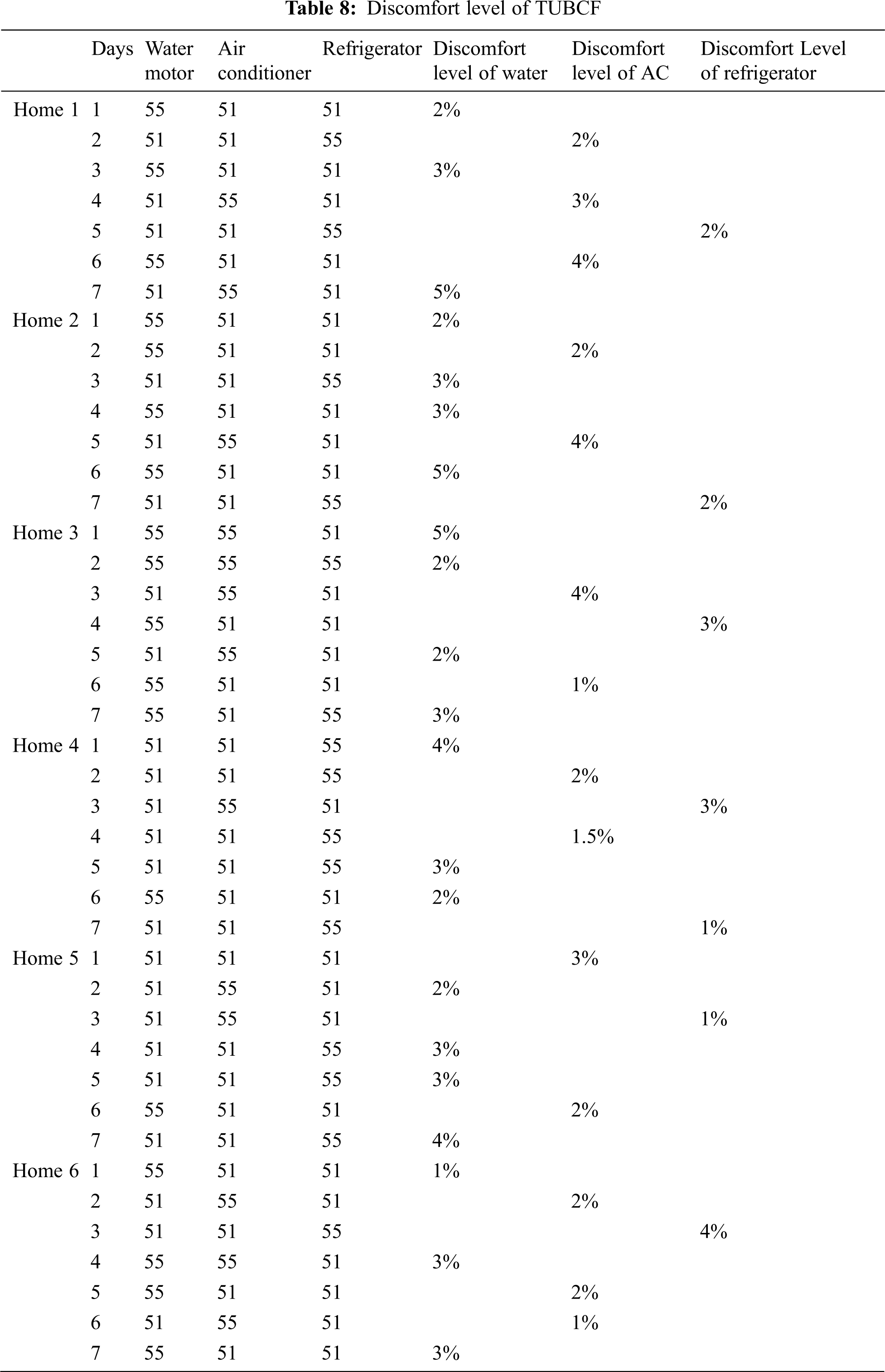
We implement a very well-known operating system concept of “CPU scheduling”, where processes are scheduled using different scheduling techniques (such as priority and round-robin) based on primitive and non-primitive properties. Therein, wait time, completion time and turnaround time will be calculated. We implement priority (non-primitive) on the CPA and TUBCF algorithms, and calculate latency, throughput time, and completion time. It is one of the most widely used scheduling methods in batch structure. Each is assigned a priority, and the process with the highest priority runs first. Since 3 devices are considered as 3 processes, we execute priority in descending order. Tab. 8 shows the level of discomfort of TUBCF algorithm.

4.3 CPA Process Scheduling

Tab. 9 details the process selection mechanism of home 6. We evenly distribute time slots equal to 15 seconds to all processes. Processes are scheduled according to descending priority, where p1 is black, p2 is red, p3 is yellow, and p4 is green. Processes arrive and are scheduled according to their priority. The main disadvantage of fixed priority is called starvation. Or block indefinitely, where processes that are ready to run the CPU can wait indefinitely due to their low priority. On a heavily loaded system, a continuous stream of high-priority processes can prevent low-priority operations from tying up the CPU forever. We find the waiting time of the device that the user has designated as yellow during peak periods.

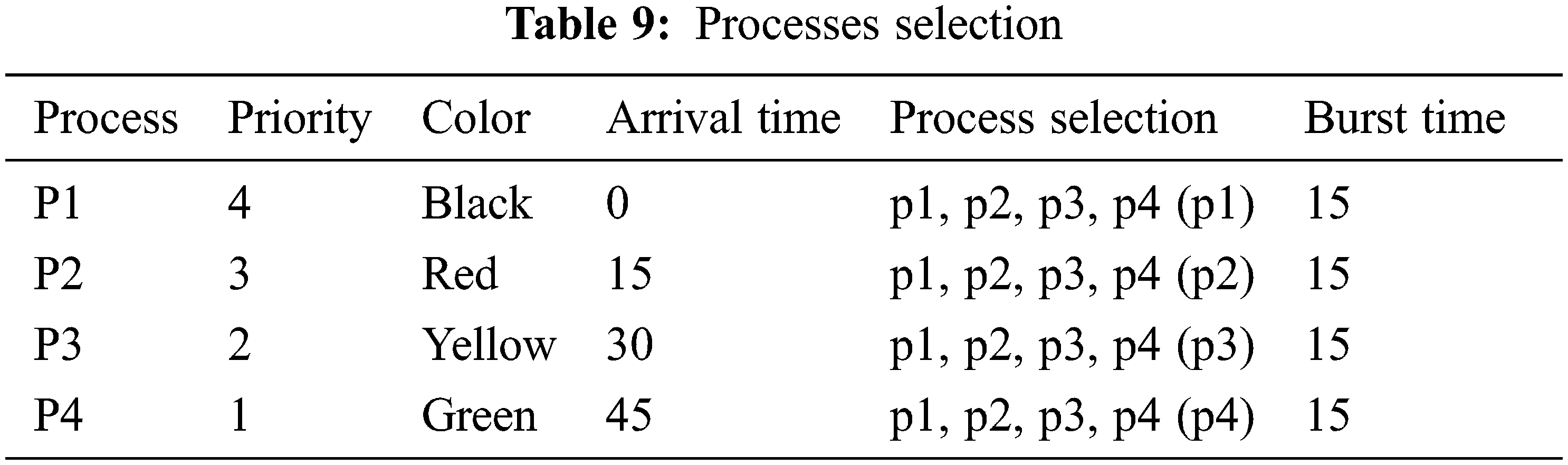
Fig. 8 shows the priority concept of CPA’s non-preemptive algorithm, during peak hours, the yellow device that has to be shut down during peak hours due to its fixed priority nature and wait time becomes longer and longer, which causes it to starve Status also increases user discomfort.

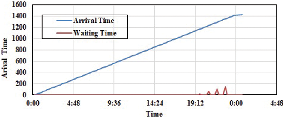
Figure 8: CPU scheduling of TUBCF algorithm

4.4 TUBCF Process Scheduling

The TUBCF process is planned according to the aging concept. Aging is a method of gradually increasing the priority of long-awaited processes in the system. For example, if the priority is between 127 and 0, we can increase the priority of the wait function by 1 every 15 min. A process with priority 127 will drop to priority 0 in less than 32 h. Likewise, in CPA, all processes are assigned the same time slot. The execution of this process depends on the time it takes for the process. If the process is not running in the first loop, increase the priority of the process. Therefore, the requirements of this process should be met and starvation issues should not appear on all devices. Fig. 9 shows that in the TUBCF case of House 6, the total device time is zero. This ensures that all devices execute without interruption and increases user convenience during busy periods.

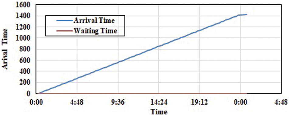
Figure 9: CPU scheduling of TUBCF

5  Conclusions

In this paper, we propose TUBCF for developing countries, a technology that can effectively reduce the inconvenience of smart grid household users equipped with smart devices during peak periods. TBUCA automatically schedules equipment according to user time requirements through aging, reducing the average peak ratio to 80%. Consumption of appliances (air conditioner, water pump and refrigerator) is charged every 15 min. For each device, we compute a utility function that selects the importance of the device in relation to the state of the system, such as temperature and water storage. After the win condition, the device with higher priority than the others will be turned on. We also implement the operating system’s scheduling concepts. A comparative analysis shows that the color performance algorithm has a longer delay for devices with user discomfort due to fixed priorities, while in our case; all devices have 0 delays due to aging, minimizing user discomfort. This work can be extended in many ways in the future. As in the context of demand response initiatives, fog and cloud-based environments can be developed to address energy management issues on dispatch to extend the comfort concept to other devices and incorporate it into the model. We can extend the experiments to different types of people and regions using different deep leering algorithms.

Acknowledgement: The authors extend their appreciation to King Saud University for funding this work through Researchers Supporting Project number (RSP-2021/387), King Saud University, Riyadh, Saudi Arabia.

Funding Statement: This work was supported by King Saud University through Researchers Supporting Project number (RSP-2021/387), King Saud University, Riyadh, Saudi Arabia.

Conflicts of Interest: The authors declare that they have no conflicts of interest to report regarding the present study.

References

 1.  D. Muthirayan, D. Kalathil, S. Li, K. Poolla and P. Varaiya, “Selling demand response using options,” IEEE Transactions on Smart Grid, vol. 12, no. 1, pp. 279–288, 2020. [Google Scholar]

 2.  M. Nizami, M. J. Hossain and K. Mahmud, “A nested transactive energy market model to trade demand-side flexibility of residential onsumers,” IEEE Transactions on Smart Grid, vol. 12, no. 1, pp. 479–490, 2020. [Google Scholar]

 3.  C. Utama, S. Troitzsch and J. Thakur, “Demand-side flexibility and demand-side bidding for flexible loads in air-conditioned buildings,” Applied Energy, vol. 285, no. 3, pp. 116418, 2021. [Google Scholar]

 4.  R. Morsali, G. S. Thirunavukkarasu, M. Seyedmahmoudian, A. Stojcevski and R. Kowalczyk, “A relaxed constrained decentralised demand side management system of a community-based residential microgrid with realistic appliance models,” Applied Energy, vol. 277, no. 11, pp. 115626, 2020. [Google Scholar]

 5.  H. R. Rocha, I. H. Honorato, R. Fiorotti, W. C. Celeste, L. J. Silvestre et al., “An artificial intelligence based scheduling algorithm for demand-side energy management in smart homes,” Applied Energy, vol. 282, no. 1, pp. 116145, 2021. [Google Scholar]

 6.  F. Naqvi, S. Iqbal and Q. U. Ain, “Energy optimization in smart buildings using intelligent fuzzy ventilation,” in Proc. ICECCE, Swat, Pakistan, pp. 1–7, 2019. [Google Scholar]

 7.  F. Javed and N. Arshad, “ADOPT: An adaptive optimization framework for large-scale power distribution system,” in Proc. ICSASS, San Francisco, CA, USA, pp. 254–264, 2009. [Google Scholar]

 8.  M. A. Arshad, S. Hasnain and N. Arshad, “A novel demand side management (DSM) technique for electric rids with high renewable energy mix using hierarchical clustering of loads,” in Proc. ICSCGICTS, Heraklion, Crete, Greece, pp. 137–142, 2019. [Google Scholar]

 9.  U. Ali, Z. A. Rana, F. Javed and M. M. Awais, “EnerPlan: Smart energy management planning for home users,” in Proc. ICNIP, Berlin, Heidelberg, Springer, pp. 543–550, 2012. [Google Scholar]

10. M. M. Hossain, K. R. Zafreen, A. Rahman, M. A. Zamee and T. Aziz, “An effective algorithm for demand side management in smart grid for residential load,” in Proc. ICAEE, Dhaka, Bangladesh, pp. 336–340, 2017. [Google Scholar]

11. A. U. Mahin, M. A. Sakib, M. A. Zaman, M. S. Chowdhury and S. A. Shanto, “Developing demand side management program for residential electricity consumers of Dhaka city,” in Proc. IEECCE, Cox’s Bazar, Bangladesh, pp. 743–747, 2017. [Google Scholar]

12. N. Kumaraguruparan, H. Sivaramakrishnan and S. S. Sapatnekar, “Residential task scheduling under dynamic pricing using the multiple knapsack method,” in Proc. ISGT, Washington DC, USA, pp. 1–6, 2012. [Google Scholar]

13. A. Barbato, A. Capone, G. Carello, M. Delfanti, M. Merlo et al., “House energy demand optimization in single and multi-user scenarios,” in Proc. IEEE ICSGC, Brussels, Belgium, pp. 345–350, 2011. [Google Scholar]

14. Z. Zhao, W. C. Lee, Y. Shin and K. B. Song, “An optimal power scheduling method for demand response in home energy management system,” IEEE Transactions on Smart Grid, vol. 4, no. 3, pp. 1391–1400, 2013. [Google Scholar]

15. C. Vivekananthan, Y. Mishra, G. Ledwich and F. Li, “Demand response for residential appliances via customer reward scheme,” IEEE Transactions on Smart Grid, vol. 5, no. 2, pp. 809–820, 2014. [Google Scholar]

16. S. Al-Rubaye and B. J. Choi, “Energy load management for residential consumers in smart grid networks,” in Proc. ICCE, NV, USA, pp. 579–582, 2016. [Google Scholar]

17. I. Shafi, N. Javaid, Y. Amir, A. Tahir, K. Naseem et al., “Home energy management using optimization techniques,” in Proc. CCISIS, Cham, Springer, vol. 772, pp. 12–24, 2018. [Google Scholar]

18. V. V. Ranade and J. Beal, “Distributed control for small customer energy demand management,” in Proc. IICSSS, Budapest, Hungary, pp. 11–20, 2010. [Google Scholar]

19. T. M. Dobrzykowski, “Feeling comfortable: A human becoming perspective,” Nursing Science, vol. 30, no. 1, pp. 10–16, 2017. [Google Scholar]

20. X. Fu, “Recommended air conditioner temperature based on probabilistic power flow considering high-dimensional stochastic variables,” IEEE Access, vol. 7, pp. 133951–133961, 2019. [Google Scholar]

21. F. Tartarini, P. Cooper, R. Fleming and M. Batterham, “Indoor air temperature and agitation of nursing home residents with dementia,” American Journal of Alzheimer’s Disease & Other Dementias, vol. 32, no. 5, pp. 272–281, 2017. [Google Scholar]

22. M. Masson, J. Delarue and D. Blumenthal, “An observational study of refrigerator food storage by consumers in controlled conditions,” Food Quality & Preference, vol. 56, no. 3, pp. 294–300, 2017. [Google Scholar]

23. R. R. Boyer and J. M. McKinney, “Food storage guidelines for consumers,” in Proc. VTB, Virginia, USA, pp. 348–960, 2018. [Google Scholar]

24. A. Lewandowska, P. Kurczewski, K. Joachimiak-Lechman and M. Zabłocki, “Environmental life cycle assessment of refrigerator modelled with application of various electricity mixes and technologies,” Energies, vol. 14, no. 17, pp. 5350, 2021. [Google Scholar]

25. M. M. Almenta, D. J. Morrow, R. J. Best, B. Fox and A. M. Foley, “Domestic fridge-freezer load aggregation to support ancillary services,” Renewable Energy, vol. 87, no. 3, pp. 954–964, 2016. [Google Scholar]

26. A. Kashif, J. Dugdale and S. Ploix, “Behavior for energy waste reduction in dwellings: A multiagent methodology,” Advances in Complex Systems, vol. 16, pp. 1350022, 2013. [Google Scholar]

27. M. Khan, H. M. Afroz, M. A. Rohoman, M. Faruk and M. Salim, “Effect of different operating variables on energy consumption of household refrigerator,” International Journal of Energy & Engineering, vol. 3, no. 4, pp. 144–150, 2013. [Google Scholar]