Multiple Extreme Learning Machines Based Arrival Time Prediction for Public Bus Transport

1  Introduction

The public delivery system is an important aspect of city transportation systems. From the perspective of the passengers, precise real-time arrival and departure information are critical to any logical transportation method as indicated by Wang et al. [1]. Electronic displays at bus stops and mobile navigation apps are two common methods for providing this information to passengers. Accurate arrival and departure information provide for shorter wait times at stations and more efficient route planning. Furthermore, accurate arrival data is required to improve the characteristics of public transportation operations in order to alter traffic movements on time via dispatch services. More individuals would use this mode of public transportation if service efficiency and wait times were improved, reducing traffic congestion on the highways. Public transportation authorities will profit from such implementations and make it easier to organize routing and scheduling activities.

The time it takes to arrive at a stop is determined by a number of factors, including the amount of time it takes to travel along segments of the transportation network, the amount of time spent waiting at stops, and delays at crossings. That is the reason why arrival time maybe taken into consideration as stochastic. Also, traffic jams, accidents, and weather situations cause additional delays. Taking into account all of the above factors, it is tough to create a version that can accurately account for various space-time elements and predicted appearance times as suggested by Islam et al. [2].

As a result, indigenous methodologies are necessary for reliable vehicle trip time predictions mentioned by Xu et al. [3]. The majority of bus journey time/arrival time prediction studies assume uniform traffic conditions. With its variability and lack of lane discipline, traffic conditions in nations like India are unique making it difficult to anticipate bus arrival times. The route considered for prediction is a 64 km long route connecting the headquarters of two districts in the southernmost part of Kerala. The intermittent places are hosts of Universities, Medical Colleges, Hospitals, Engineering/Polytechnic Colleges, Sports Centers, Courts, Arts Colleges and many Government offices. So regular commuters travel on this route up to a distance of 64 km in the morning for work and in the evening back to their residence and vice versa. The transit vehicles consist of local buses, fast/nonstop passenger buses and even luxury buses with limited stops to increase transport utility. At present, a passenger waiting at an intermediate stop has no facility to see when the bus of his choice would turn up or even whether a particular bus in the route is plying that day or not. After a long wait for a particular bus, one will rely on some local buses to reach the destination. Even if the bus of one’s choice is getting delayed, there is no way to track the late arrival. The probability is that you get a bus of your choice or may not get it. Hence as far as the utility of time is considered, it is a big question. So many passengers resort to their own means of transport increasing cost, traffic and more vehicles on the road leading to pollution and congestion. There are three intermediate bus stations in this 64 km route. Even if approaching a bus station, a person has no means to track the bus. Hence, boards displaying the bus id and arrival time of the buses at bus stations will be of great use to transit passengers. Kerala State Road Transport Corporation (KSRTC) buses are the main transport means for the public on this route. Buses start from Thiruvananthapuram central station, end their trips at Kollam and ply back to Thiruvananthapuram. There are long-distance buses to other parts of the state for which this route forms a middle part. KSRTC is the backbone of the public transportation system of Kerala. This is established by the fact that the number of passengers utilizing the public transportation system from different bus stations under Thiruvananthapuram district alone is 9,151,898 during this period 2015–2018 as analyzed by Leejiya et al. [4].

The nature of the bus pattern is that there maybe two or three buses starting from the origin within a gap of say 5 min and after that subsequent buses around 15 min later. This gap of 15 min will change the whole traffic scenario as far as morning peak time from 8 to 10 am and evening peak time from 4 to 6 pm is considered. Hence, the significance of bus arrival prediction. Regular passengers will have their buses of choice. One waiting after work at a particular bus stop can search his mobile App for a particular bus by entering the bus id. For instance, the bus can be 10 km away that day/time. The GPS unit on the bus will regularly send the bus location details to the server. On receiving a request from the user, the server calculates the time it takes for the transport to reach that place considering the present data and how the traffic will be from the historical data for the day of the week and weather conditions for which the network is trained. The predicted arrival time can be displayed to the user in his mobile App or through SMS. Also, display boards at major bus stations can be updated with the arrival times of approaching buses so that one can plan their trips accordingly. The accuracy of bus predictions depends on many factors. Even if an approaching bus is 5km away, it may take (1 min to travel 500 m), say 10 minutes in the early morning to cover this distance. The same distance can only be covered in 20 min in the morning peak and evening peak hours. This delay can be included in the prediction only by considering the traffic pattern obtained from the historical data. Hence, the need for prediction.

In public transportation networks, many ITS technologies have been widely deployed. Machine learning algorithms are helpful for determining bus travel times when the associations between travel time and traffic parameters involved are nonlinear and obtained through ICTs. The trip duration of buses varies significantly due to the varying traffic flow and the impact of signals at the intersection, reducing the stability of public transportation. For greater accuracy of timetable operation, a number of alternatives are presented, tested, and compared. Passengers are informed of bus arrival times, allowing for consistency in passenger waiting times.

The structure of the paper is as follows. In Section 2, the related works in this area are explained. In Section 3, the proposed work is explained with the block diagram scientifically. The results and discussion with numerical analysis and tables are explained in Section 4. Section 5 concludes the paper.

2  Related Works

Previously numerous works have been proposed to perform the arrival time prediction. Arrival time prediction is done by considering various linear and nonlinear route parameters. Numerous classification and prediction algorithms are used to perform an efficient determination of accuracy. Some of the prior works which are done to perform the arrival time prediction are explained as follows.

According to Zhang et al. [5] bus arrival time is commonly forecasted to assess future bus operation conditions (e.g., bus bunching and transit service reliability) and can then be used to inform present control actions, particularly for real-time control systems. The time of travel and traffic scenario are the most important components in forecasting, yet most previous techniques have only looked at the impact of signal control on delay in travel time. Using data from actual studies in Jinan City between bus stops with signalized junctions, the observed bus journey time is compared to the predicted trip time. According to the findings, this model has a low mean relative error.

The arrival time of public vehicles to transportation stops, according to Agafonov et al. [6] is critical for travel planning since it aids in reducing halt wait times and selecting the best alternate route. This study investigates the LSTM neural network’s capacity to predict the arrival time of public transportation. This method considers diverse information about the transportation situation by including statistical and actual traffic flow data. The model is being evaluated using data from bus routes in the Russian city of Samara. Chen et al. [7] suggested an Arrival Time Prediction Method (ATPM) based on Random Neural Networks (RNN). The average accuracies of RNNs for highway and urban routes, respectively, were found to be 94.75 and 78.22 percent in trials. Furthermore, the proposed ATPM has higher accuracy than earlier data mining approaches.

To increase the accuracy of real-time public transportation information, Cai [8] presented a prediction model based on physical systems architecture. The overall bus trip time was split into three components in the model: running time, dwell time, and intersection delay time, with data divided into three categories: historical data, static data, and real-time data. In the collaborative layer, real-time data from the perceptual layer was combined with past data from the collaboration layer to compute the bus arrival time. When comparing the model findings to the actual results, it was shown that the model can meet the criteria for bus arrival prediction.

Jiber et al. [9] conducted a road traffic forecast study in Morocco using data from the Moroccan center for road studies and research. They merged Ensemble-based ELM approaches based on the number of neurons in the hidden layer. According to the study, the technique is more accurate than ELM alone in terms of providing value.

Zhao [10] developed a forecasting model for distributing passenger flows over multiple routes and trains. The method presented in this research is used to analyze the Shenzhen metro system. The first form of data used is smart card transaction data, which is received when a passenger taps their smart card to pass through an entrance or departure gate, and train operating details, which are created when a train arrives or exits a station. Maximum likelihood estimation was also used to calculate two types of time-dependent polynomial distributions.

Multiple hidden layers ELM network structure, according to Xiao et al. [11] improves the average accuracy of prediction in comparison with ELM and two hidden layered ELM structures. This method uses a component of the TELM algorithm, which uses the inverse activation function to produce hidden layer parameters, and inherits the feature of standard ELM, which randomly initializes the weights and bias. The real hidden layer output is then compared to the expected hidden layer output, and the actual output is calculated using the parameters established above. This method reduces the MSE (mean square error) in regression issues.

Above mentioned techniques have both advantages and disadvantages. The major disadvantages of the previous works are the complex real-time data collection process and the feature extraction process. The main purpose of this work is to overcome the shortcomings of the previous work.

•   To reduce the complexity of the data collection and updating of corresponding datasets.

•   To improve the accuracy of the prediction process maintaining the minimum feature extraction technique.

•   To reduce the complexity of the arrival time prediction and increase the capability of the real-time testing process.

Detailed information on the implementation of the proposed technology is presented in the following sections.

3  Bus Arrival Time Prediction Using MELM

The ELM has the potential to handle big data. ELM is implemented completely automatically as there is no necessity for iterative tuning and external intervention is not required. Hence ELM has the advantage of fast learning speed.

The number of hidden nodes, including weights between the input layer and the hidden layer and the bias of the hidden layer neurons can be assigned independently. The hidden layer output matrix is estimated and finally obtains the weight between the hidden layer and the output layer [12]. Thus, the output weights of the network can be analytically calculated by the simple generalized inverse operation. It can be represented as a (n × m) matrix with n < m, which need not be a square matrix. Here we have more unknowns than we have equations.

In these conditions, there are many possible values for x that make Ax = y. We need to find such a solution x of minimum (weighted) Euclidean norm, i.e., of minimum ∣∣x∣∣. Pseudo-inverse is basically an inverse of any type of matrix (square or non-square).

Fig. 1 shows the ELM structure which includes d input layer neurons, L hidden layer neurons, and m output layer neurons. First, consider the training sample {X, Y} = {xi, yi–} (i– = 1, 2,…., Q), and there is an input feature X = [xi1, xi2, …., xiQ] and the desired matrix Y = [yj1, yj2, …., yjQ] comprised of the training samples. Second, the output of the hidden layer can be represented as an activation function H,

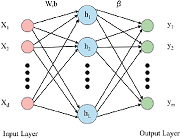
Figure 1: Structure of ELM

H=g(wX+b) (1)

where H represents the hidden layer output, w represents the weights between the input layer neurons and hidden layer neurons and b is the bias of the hidden layer neurons randomly assigned.

Third, the ELM assumes β as the weights between the hidden layer and the output layer neurons. We get

Hβ=T′ (2)

where T′ is the transpose of T. In order to obtain the unique solution with minimum error, we use the least square method to calculate the weight matrix values of β.

β=H+T′ (3)

In order to generalize the network and make the results more stable, we add a regularization term β. In the case where the number of hidden layer neurons is smaller than the number of training samples,

β=(1/λ+HTH)−1HTH′ (4)

If the number of hidden layer nodes is greater than the number of training samples,

β=H(1/λ+HHT)−1T′ (5)

ELM may not reach the optimal classification limit since the nodes remain unchanged during the training process. Therefore, samples closest to the classification limit may not be classified correctly. ELM has been able to improve sorting performance, reduce the number of misclassified samples, and reduce variation between different implementations.

For a learning set, the number of hidden layers can be varied between 80 and 360 to determine the optimum performance. Increasing the number of hidden nodes in an ELM leads to the development of excessive overfitting in the model. Another critical factor that influences the performance of the ELM is the accuracy with which the output weight is calculated. Attempts have been made to increase the resilience and stability of ELM as a consequence of these two features. In order to avoid overfitting in ELM, Biased Drop Connect and Biased Dropout regularization can be used as suggested by Jieand et al. [13]. As a consequence, it is crucial to choose an ELM that is appropriate for the number of hidden nodes present according to Zhao et al. [14].

A) Block Diagram

Multiple ELMs (MELM) are proposed to predict the arrival time for public transportation based on bus parameters and road parameters. The block diagram consists of three databases such as trajectory, dynamic and road databases. Trajectory data is the sequence of information about the route where each data point represents the GPS location of the stop, the GPS location of the traffic signal post and the arrival time of the bus at the bus stop according to He et al., [15]. Dynamic data contain the data from the cloud server which has to be updated for example the weather data and traffic data from the cloud. The road data is the static data that holds the information about the road such as the number of curves and up’s and down’s that are present in the particular route of the road.

Three separately trained ELM classifiers are used to process these data for highly accurate results. The block diagram in Fig. 2 shows the overall workflow of the proposed bus arrival time prediction using MELM.

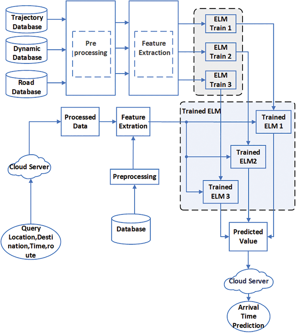
Figure 2: Block diagram of bus arrival time prediction

B) Parameters Considered

▪ Distance (D)

▪ Waiting Time at Stops (WTS) or Dwell Time

▪ Red signal Duration at Traffic Signal (RSD)

▪ Traffic Density (TD)

▪ Turning Density (TRD)

▪ Rush hours (RH)

▪ Weather conditions (WC)

▪ Number of passengers on the bus (NP)

▪ Type of day

▪ Road Type (RT)

▪ Average Vehicle Speed limit (AVSL)

▪ Current vehicle speed

Bus parameters are data acquired from the bus such as average vehicle speed and number of passengers. Route parameters are data collected from the route such as the number of stops, road type and rush hour information. Also, traffic density along different bus line segments for distinct times of travel varies and hence, traffic density has an important impact on arrival time prediction. The approach takes into account dwell time at stops also.

C) Data Preparation

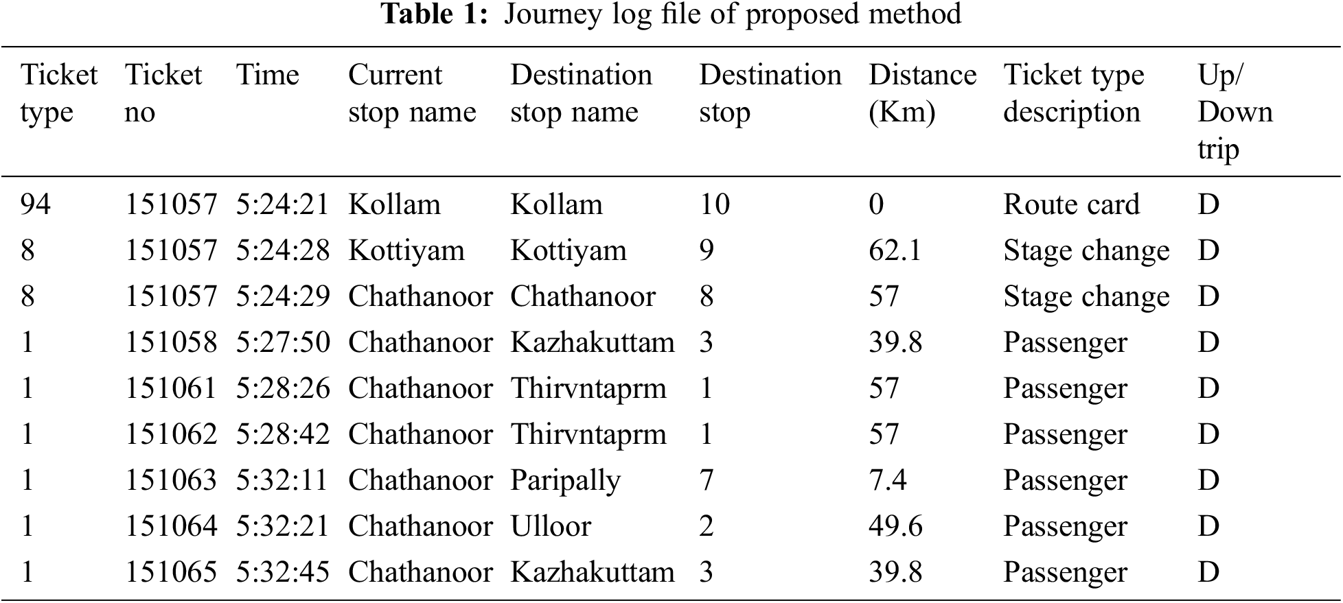
The tests are being carried out on the road network between Kollam and Thiruvananthapuram, which comprises signal and road trajectory sections. The data from live bus arrivals and departures is merged to produce a bus path dataset. The suggested approach was built using bus trajectory data from 1st March to 31st March, 2021. The journey log file used in the proposed approach is shown in Table 1, and it contains passengers with a current time-based stop to destination stop.

The use of road network is used to determine the position of junctions and the number of traffic lights along a certain trip route. The ID (a three-digit number) of each bus stop in sequential order, as well as the GPS position (latitude and longitude) of each bus stop, are included in the bus route information. It is possible to create a bus trajectory dataset using real-world bus arrival time data.

The dataset for training with bus route number 515 is depicted in Fig. 3. The real-time data set from KSRTC obtained comprising of the desired parameters is depicted in it. The data acquired for the period from 1st March 2021 to 31st March 2021 is used for training the MELM, and the data from 1st June 2021 to 7th June 2021 is used for comparison with the predicted results.

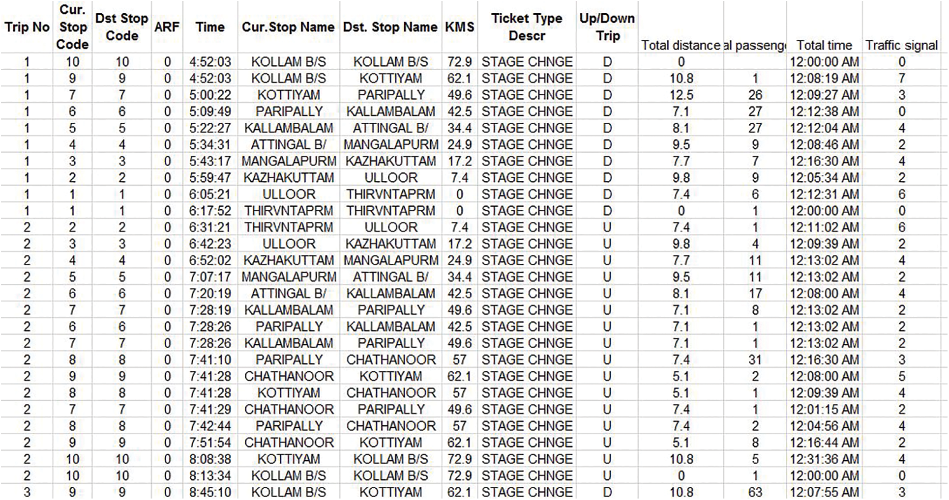
Figure 3: Data set for MELM training

D) Feature Extraction and Analysis

Feature extraction extracts the parameters that influence the bus trip time on the selected bus line. All of the important parameters that boost prediction performance are deduced here. When a collection of bus routes is generated, each collection comprises routes that cover a different day of the week than the one before it. This is done to prevent routes from being duplicated between groups. Time is divided into one-hour pieces for each group, and travel time is estimated by averaging all trajectories whose journey start time falls inside the groups given time period. Trips that begin at different times of the day on the same day have dramatically varied travel schedules. As a result, the trip time distribution differs between weekdays and weekends, with Sunday having the best travel conditions compared to other days.

i) Prediction on Waiting Time

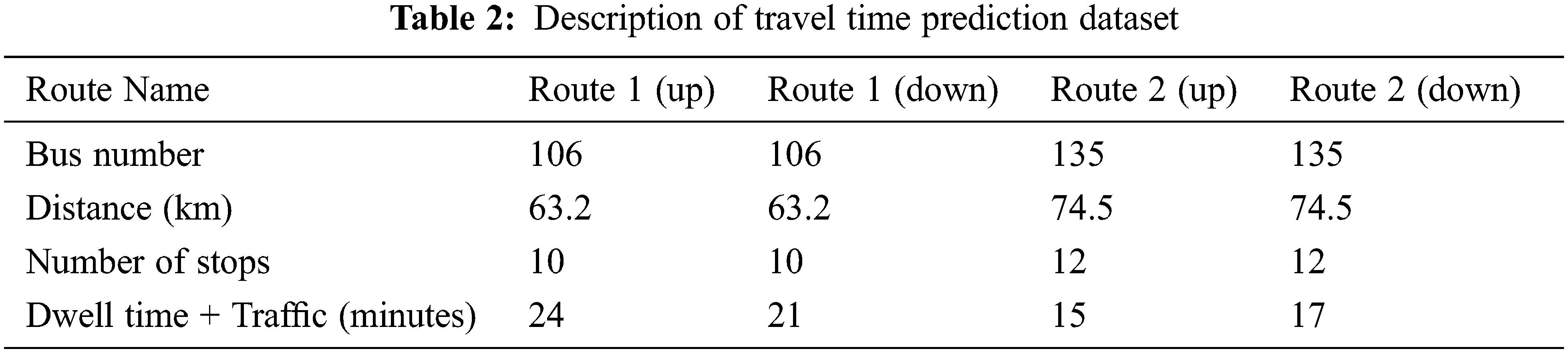
The overview of the travel time prediction dataset with route details such as traffic intensity, distance and the number of stops is provided in Table 2. With increasing journey length, the values of the above components appear to become more stable, leading to greater accuracy in prediction of the outcome.

ii) Performance Metrics

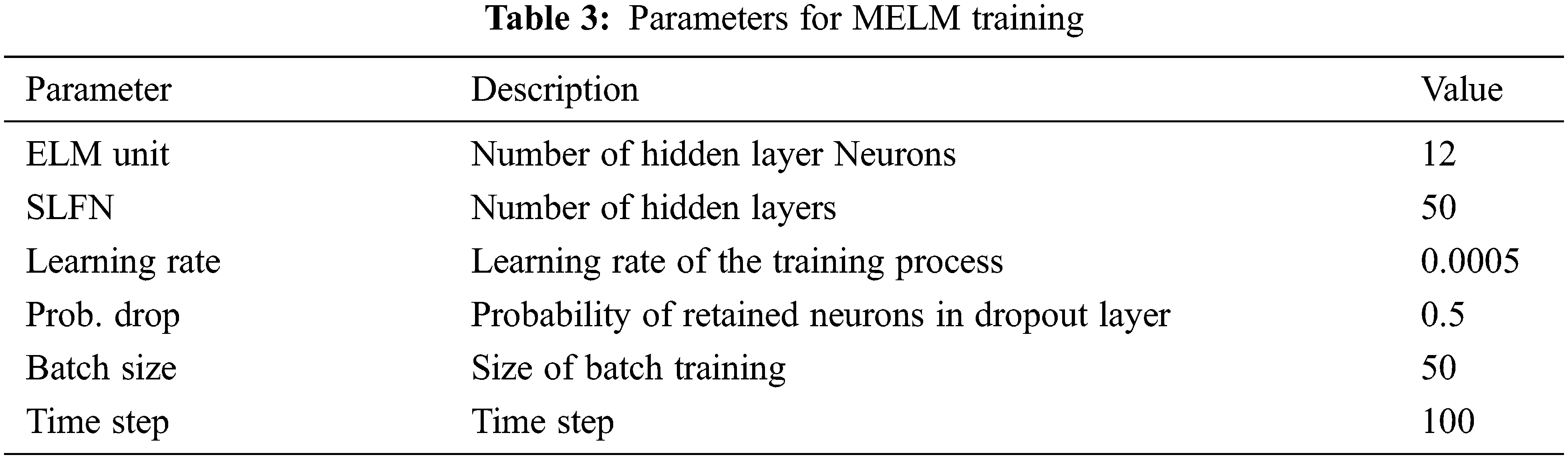
The MELM is trained with historical data obtained from KSRTC and simulations are carried out using MATLAB R2021a. The parameters considered for MELM training are depicted in Table 3. The ELMs used for structuring the MELM consist of 12 hidden layer neurons. The model is tested with 50 hidden layers. To prevent overfitting the dropout is set at 0.5. This is done for each of the ELM layers. The training process is repeated for fifty epochs. The output layer yields the predicted output.

4  Results and Discussion

The suggested method proposes a novel strategy for processing various aspects impacting traffic for bus arrival time prediction that employs multiple ELMs. All twelve elements that have a major impact on bus arrival times are analyzed. MAE, MAPE, and accuracy are used to assess the situation. The discrepancy of actual time from MELM’s expected arrival time was calculated using error values.

A. Performance Measures

The performance measures used are Mean Absolute Error (MAE) and Mean Absolute Percentage Error (MAPE). Besides MAE and MAPE, also the average error is calculated for travel time per km (MAE/distance).

Mean Absolute Error (MAE): MAE between matched sets of data that reflect the same event is a statistical measure of error. Comparisons between planned and observed data, as well as measurement procedures are made.

MAE=∑I=1N⁡|YI−XI|N (6)

where YI is the predicted value, XI the true value and N is the number of samples.

Mean Absolute Percentage Error (MAPE): It is a statistical measure of a forecasting approach’s efficiency in predicting the future.

MAPE= 100N∑T=1N⁡|AT−FTAT|    (7)

where AT is the actual value and FT is the forecast value and N is the number of fitted points.

Historical Average (HA) is a prediction method representing the average value of physical quantity over a period of time and is a baseline for travel time prediction. The predicted travel time is the average of all historical travel records of the same period that have the same origin and destination, given the origin, destination and journey start time.

Table 4 shows the comparison of the absolute mean error, absolute mean percentage error concerning the different routes. The Proposed method shows fewer errors compared to the existing methods. Fig. 4 shows the performance comparison of the existing methods with the proposed method and the proposed method outperforms the existing methods.

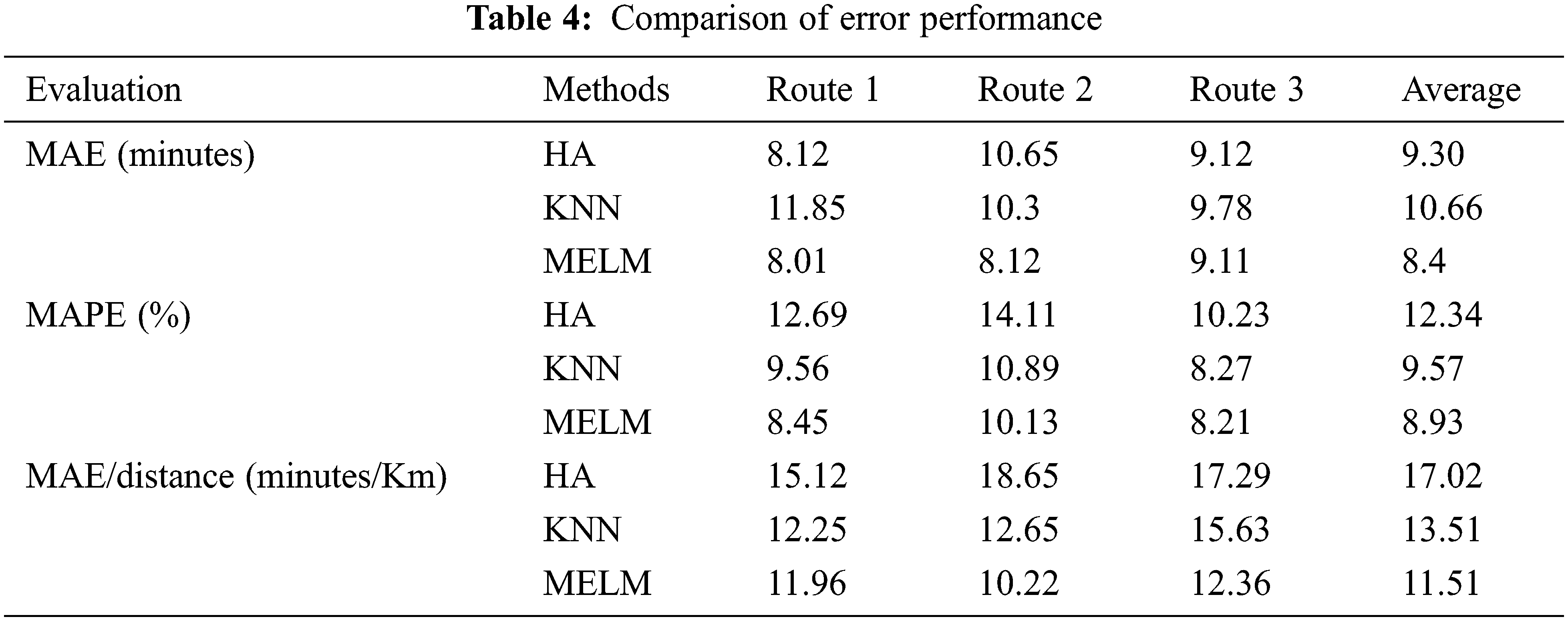
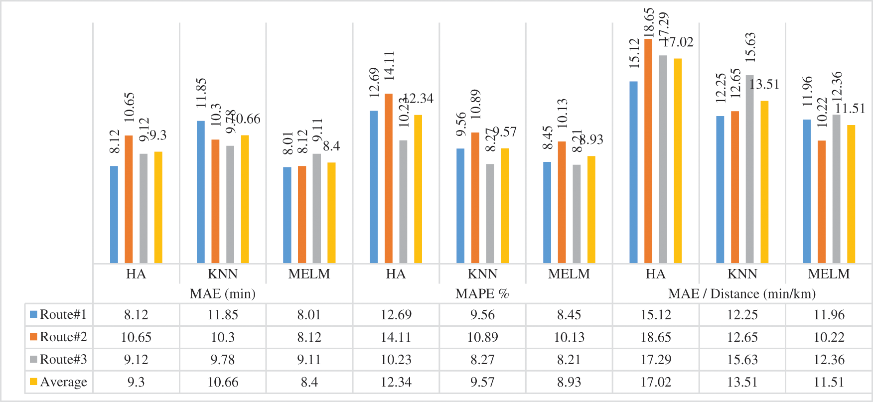
Figure 4: Performance comparison with existing methods

B. Performance Analysis based on simulations of Prediction using MELM

MATLAB R2021a was used to assess the MELM performance using real-time data from 1st March 2021 to 31st March 2021 for training and 1st June 2021 to 7th June 2021 for testing.

Fig. 5 shows the prediction performance of the suggested MELM with ELM.

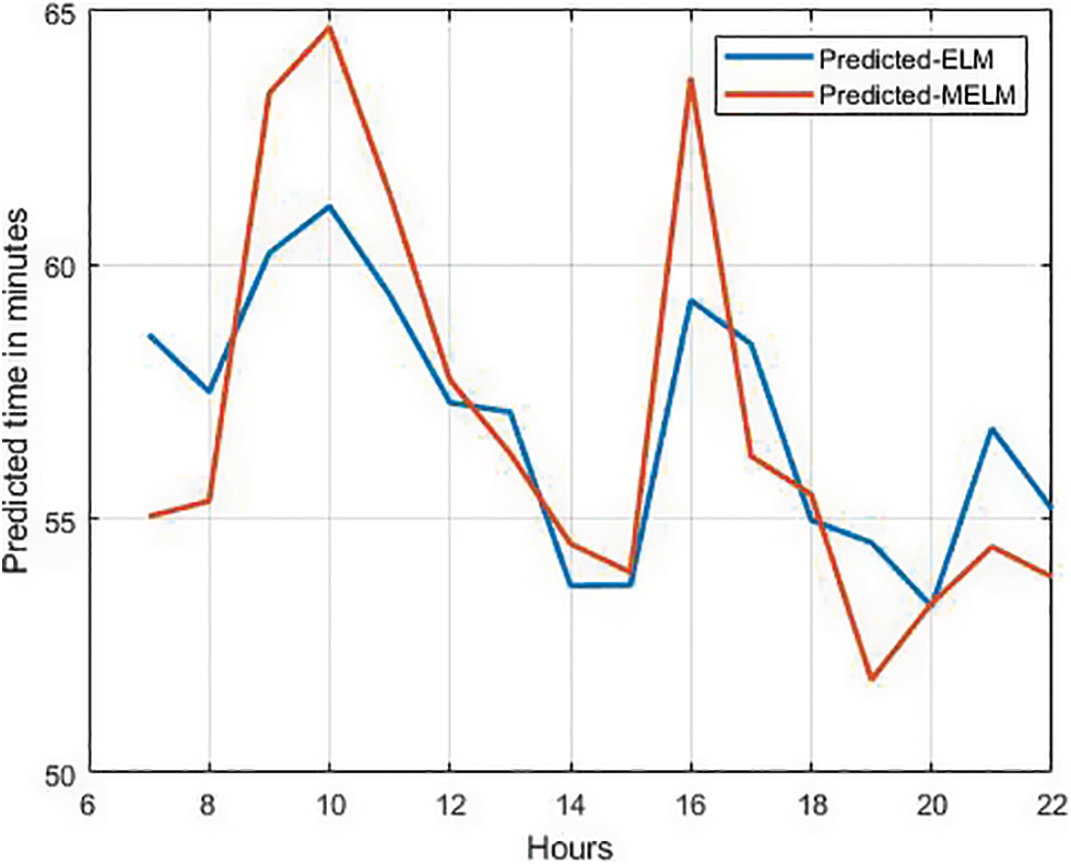
Figure 5: Performance comparison of ELM and MELM based on predicted time

MAE of ELM and MELM is compared in Fig. 6.

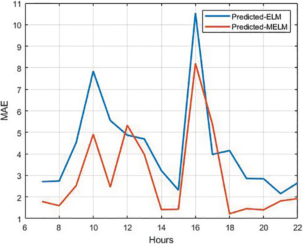
Figure 6: Performance comparison of ELM and MELM based on MAE (minutes)

Fig. 7 compares the percent MAPE performance of ELM and MELM.

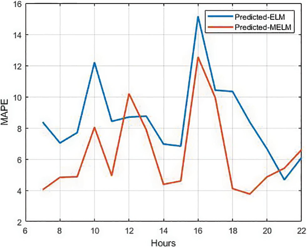
Figure 7: Performance comparison of ELM and MELM on % MAPE

Table 5 demonstrates the evaluation performance for various time periods based on simulations with ELM and MELM. Because journey times are connected with variable degrees of traffic uncertainty, travel needs at stops, and so on, MAE, MAPE, and accuracy vary significantly during different time periods of a day for both techniques. For the time period 9 to 11 am, MAE is less than half a minute (0.28 min) slower than MELM. MAE is as high as 4.67 min in the case of ELM prediction for the same period. The MAE of the ELM approach is still high compared to MELM on the test route with a travel time of 110 min. From the results, 2 to 6 pm is the interval in which MELM exhibits average results compared to other periods.

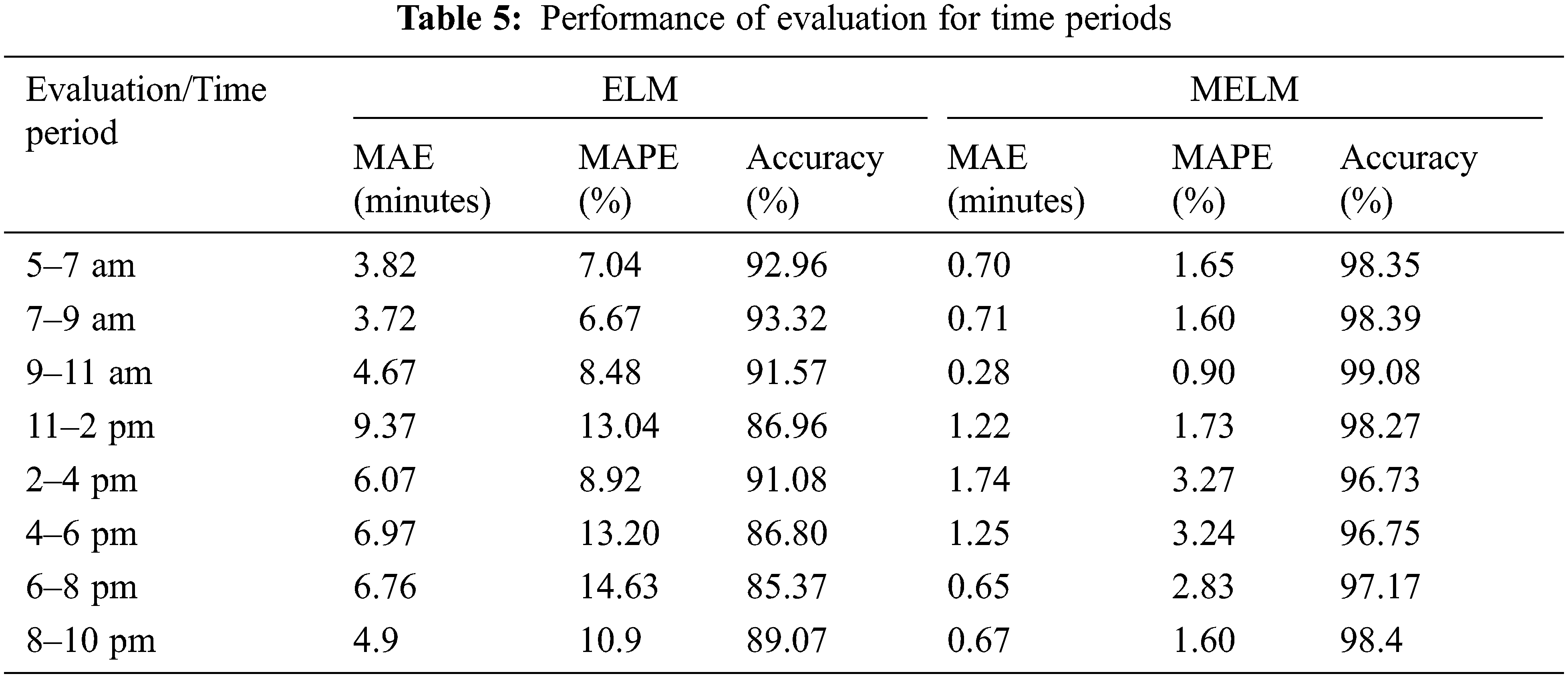
The average variation between anticipated times by ELM is between 3.82 and 9.37 min, according to the results. The average inaccuracy in MELM is only 0.28 to 1.74 min in both the up and down routes. The error in all MELM performance predictions is less than one minute, and the accuracy is up to 99 percent. As a result, the proposed strategy of using MELM to anticipate bus arrival time for public transportation networks is a better approach.

C. Performance Comparison of Proposed Method

The proposed MELM is used in a simulated investigation of accuracy prediction utilizing traditional approaches such as ANN, SVM, and ELM. Fig. 8 shows the simulation results for accuracy, which show that MELM has the best accuracy. From 11 am to 2 pm, accuracy is at its peak, ranging from 98.27 to 99 percent.

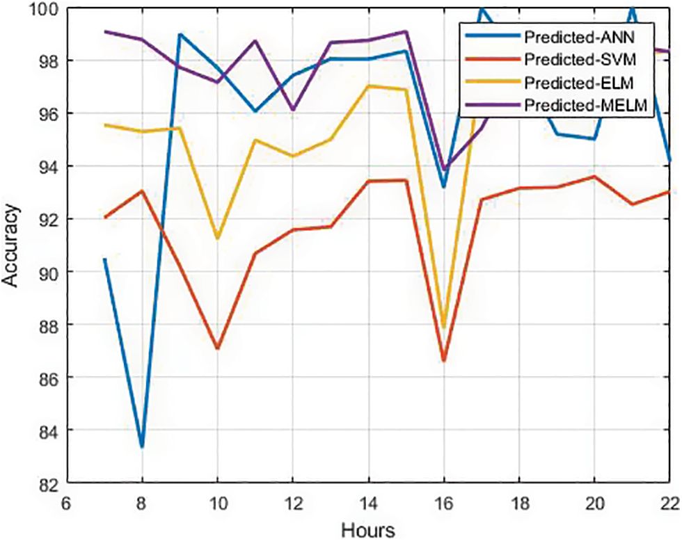
Figure 8: Accuracy comparison (%)

A comparison of MAE is done as displayed in Fig. 9. MAE varies between 0.28 to 5.7 min for MELM. There is significant variation in MAE for arrival time predictions with other approaches compared to MELM.

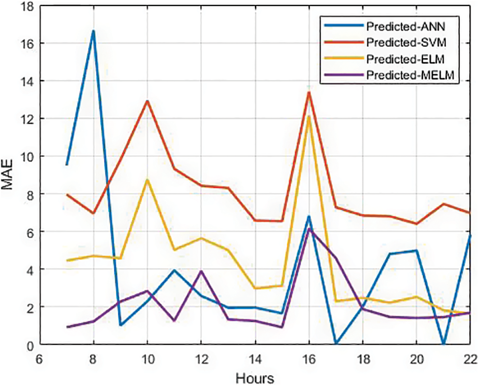
Figure 9: MAE comparison (minutes)

The performance of ELM and MELM predictions of this work was compared to that of ANN and SVM predictions performed in the research titled “Prediction of Bus Travel Time Over Unstable Intervals between Two Adjacent Bus Stops” by Mansur et al. [16] as shown in Fig. 10. The time between 9 and 11 am shows more relative errors, the proposed MELM method exhibits low error value compared to the other approach.

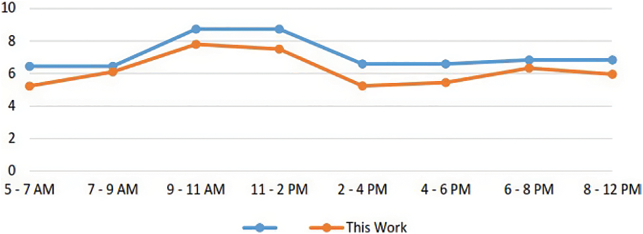
Figure 10: Comparison of arrival time with error (minutes) over unstable intervals of MELM with Mansur et al. [16]

Table 6 compares accuracy on normal days and weekends, while Table 7 compares accuracy on festival days and during rainy weather. The simulation methodologies for weekdays and weekends have considerable variances in accuracy. Weekday prediction accuracy is lower than weekend prediction accuracy with ELM. This is due to the enormous number of vehicles on the road and the stochastic nature of traffic. During weekends, the accuracy of ELM forecast has also improved. As seen in Fig. 11, the MELM technique has the best accuracy on weekdays. When comparing MELM to ELM for weekends, there is a corresponding increase in accuracy. In this prediction also accuracy is least for early afternoon with MELM.

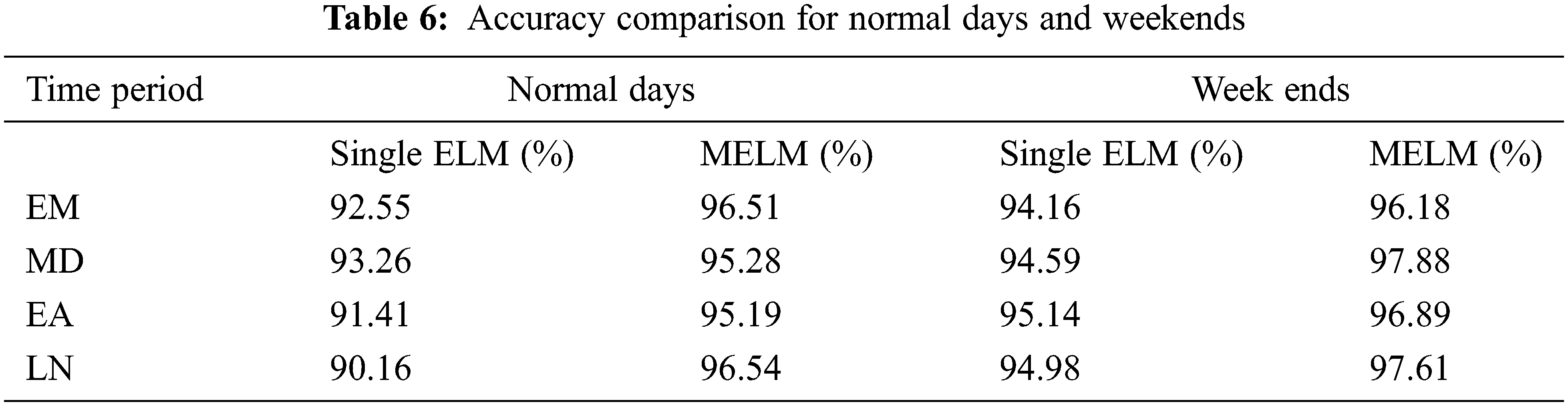
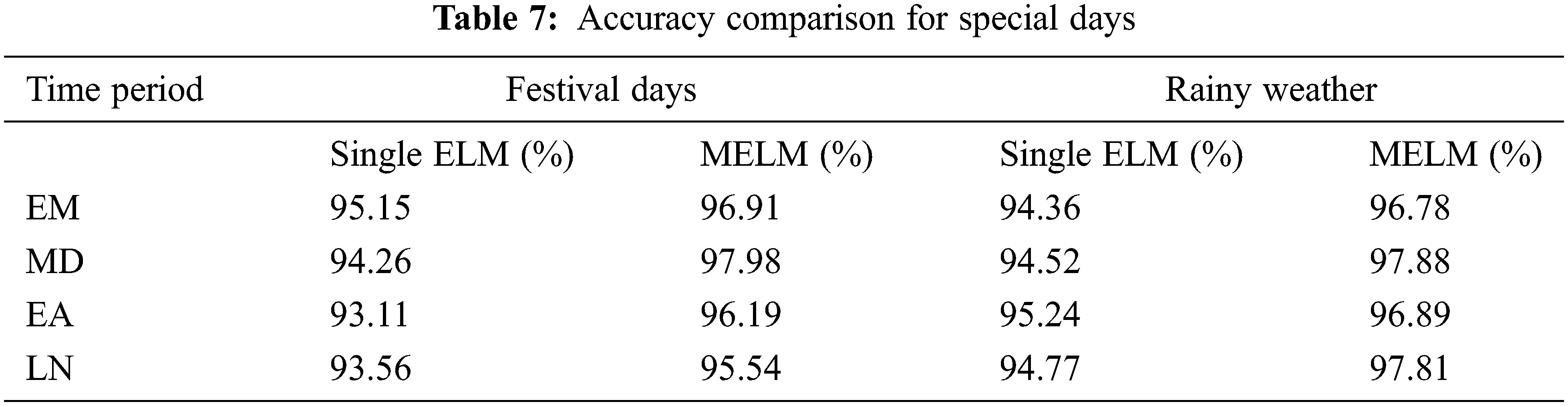
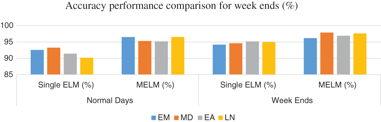
Figure 11: Accuracy comparison for normal days and weekend

Simulation comparison is also done for festival days and rainy weather conditions with the proposed approach. From Fig. 12 it is seen that MELM maintains its universal approximation capability even during adverse weather conditions.

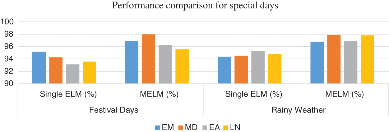
Figure 12: Accuracy comparison for special days

5  Conclusion

The study found that by combining current bus location with stochastic traffic information and variations in demand with time and day, the MELM technique can accurately predict bus arrival time. To address the trade-off that exists between different machine learning algorithms, improved prediction methods are offered. The proposed system has the advantage of higher accuracy and faster calculation with vast and complicated non-linear data. The value of public transportation systems is increased by including dynamic and accurate travel information systems.

The suggested model takes advantage of ELM’s viability and application in the area of trip time forecasting. According to the findings, bus utilization can be anticipated, and daily bus travel can be predicted with more accuracy. In comparison to other methodologies, research has shown that MELM is superior in terms of accuracy and error for arrival time forecasts. With an MAE of less than one minute, the suggested MELM achieves an accuracy of up to 99 percent. As a result, MELM is the most effective method for predicting bus arrival times in public transportation systems. The estimated trip time can be utilized to deliver real-time bus arrival information to the general public via web pages, smartphone apps, and public display boards.

Funding Statement: The authors received no specific funding for this study.

Conflicts of Interest: The authors declare that they have no conflicts of interest to report regarding the present study.

References

1. L. Wang, Z. Zhongyi and F. Junhao, “Bus arrival time prediction using RBF neural networks adjusted by online data,” Procedia-Social and Behavioral Sciences, vol. 138, no. 1, pp. 67–75, 2014. [Google Scholar]
2. M. R. Islam, M. Hadiuzzaman and M. Banik, “Bus service quality prediction and attribute ranking: A neural network approach,” Public Transport, vol. 8, no. 1, pp. 295–313, 2016. [Google Scholar]
3. H. Xu and J. Ying, “Bus arrival time prediction with real-time and historic data,” Cluster Computing, vol. 20, no. 4, pp. 3099–3106, 2017. [Google Scholar]
4. J. Leejiya and A. Jisha, “Performance evaluation of kerala state road transport corporation,” International Journal of Engineering Research & Technology, vol. 8, no. 6, pp. 1–15, 2019. [Google Scholar]
5. H. Zhang, S. Liang and R. Leng, “A prediction model for bus arrival time at bus stop considering signal control and surrounding traffic flow,” IEEE Access, vol. 5, no. 1, pp. 127672–127681, 2020. [Google Scholar]
6. A. Agafonov and A. S. Yumaganov, “Bus arrival time prediction using recurrent neural network with LSTM architecture,” Optical Memory and Neural Networks, vol. 28, no. 3, pp. 222–230, 2019. [Google Scholar]
7. H. Chen and C. Hua, “An arrival time prediction method for bus system,” IEEE Internet of Things Journal, vol. 5, no. 5, pp. 4231–4232, 2018. [Google Scholar]
8. X. S. Cai, “Collaborative prediction for bus arrival time based on CPS,” Journal of Central South University, vol. 21, no. 3, pp. 1242–1248, 2014. [Google Scholar]
9. M. Jiber and A. Mbarek, “Road traffic prediction model using extreme learning machine: The case study of Tangier, Morocco,” Information, vol. 11, no. 12, pp. 542–551, 2020. [Google Scholar]
10. J. Zhao, “Estimation of passenger route choice pattern using smart card data for complex metro systems,” IEEE Transaction on Intelligence Transport System, vol. 18, no. 4, pp. 790–801, 2017. [Google Scholar]
11. D. Xiao and B. Li, “A multiple hidden layers extreme learning machine method and its application,” Mathematical Problems in Engineering, vol. 1, no. 8, pp. 1–10, 2017. [Google Scholar]
12. G. B. Huang, Q. Y. Zhu and C. K. Siew, “Extreme learning machine: Theory and applications,” Neurocomputing, vol. 70, no. 1, pp. 489–501, 2006. [Google Scholar]
13. L. Jieand and W. Xiaodan, “BD-ELM: A regularized extreme learning machine using biased dropconnect and biased dropout,” Mathematical Problems in Engineering, vol. 11, no. 9, pp. 72–85, 2020. [Google Scholar]
14. X. Zhao and Z. Zhen, “A novel recommendation system in location-based social networks using distributed ELM,” Memetic Computing, vol. 10, no. 3, pp. 321–331, 2018. [Google Scholar]
15. P. Qingwen and G. Ling, “Travel-time prediction of bus journey with multiple bus trips,” IEEE Transactions on Intelligent Transportation Systems, vol. 20, no. 11, pp. 4192–4205, 2018. [Google Scholar]
16. A. Mansur, M. Tsunenori and Y. Tsubasa, “Prediction of bus travel time over unstable intervals between two adjacent bus stops,” International Journal of Intelligent Transportation Systems Research, vol. 18, no. 1, pp. 53–64, 2020. [Google Scholar]
Cite This Article
Copyright © 2023 The Author(s). Published by Tech Science Press.
This work is licensed under a Creative Commons Attribution 4.0 International License , which permits unrestricted use, distribution, and reproduction in any medium, provided the original work is properly cited.
Downloads
Citation Tools