Backstepping Sliding Mode Control Based on Extended State Observer for Hydraulic Servo System

1  Introduction

Hydraulic servo system has become increasingly popular in modern industrial automation and has been used in many fields [1–3], including aircraft actuators [4], rolling mills [5] and load simulators [6]. Compared to their electrical or pneumatic counterparts, hydraulic system demonstrates excellent superiorities of high precision, fast response, large power density, and compact structure [7–9]. However, precision motion control of hydraulic servo system is very hard due to inherent nonlinearities, time-variant loads, parametric uncertainties and uncertain disturbances [10–12]. In view of these drawbacks, how to achieve high precision control of hydraulic servo system has attracted great attentions in both academia and industries over the last decade. Although the traditional constant-gain controllers based on linear model are relatively mature, their global stability and tracking accuracy can hardly meet the real-time control requirements of modern industries [13]. Therefore, it is indispensable to build a dynamic mathematical model and design an advanced controller to improve the tracking performance and anti-interference ability of hydraulic servo system.

To obtain satisfactory control performance, many control methods have been developed, such as PID control [14], adaptive control [15], robust control [16], sliding mode control [17], fuzzy logic control [18] and backstepping control [19]. The classical PID control is widely used in hydraulic servo system for its simple structure, clear function and easy realization. Nevertheless, strong nonlinearity and parameter uncertainty reduce the control performance when the operating point of the system changes [20]. Concerning that PID controller fails to solve the parameter variation and external disturbance, adaptive control is proposed to cope with variable working conditions due to its excellent online learning ability [21]. However, it is difficult for adaptive control to guarantee the system stability because the uncertain parameters of hydraulic servo system need to be linearized before they are processed [22]. That is to say, the nonlinear system is first transformed into the equivalent linear system by canceling out the nonlinear terms using feedback method [23]. Then, the mature linear control methods can be used in the nonlinear system. To further solve nonlinearities and uncertainties that cannot be presented in a linear parameter form, function approximation and fuzzy rules are adopted to approximate the matched and mismatched uncertainties [24–26]. However, the heavy computation burden and complicated convergence analysis restrict the practical application of adaptive control [27]. In order to effectively reduce the chattering of sliding mode control, the discontinuous sign function can be replaced by continuous functions, such as saturation functions, hyperbolic functions and switching functions [28–30]. The robust controller can guarantee a prescribed transient tracking performance and final tracking accuracy in existence of both modeled and unmodeled dynamics. However, the robust term adopting fixed boundaries rather than specific dynamic boundaries to roughly compensate for unmodeled dynamics makes the robust controller too conservative [31].

Compared to other control methods, backstepping control has attracted great interests due to its robustness to external disturbances and low sensitivity to parameter variations. As backstepping control implies, the high-order nonlinear system is decomposed into multiple first-order systems. The variables at the next step are taken as virtual input and acted on the current subsystem, and the Lyapunov function is established according to the system at the upper step to achieve system stability. Until the last step, the true control expression and the actual update law are obtained. To avoid the differential explosion of traditional backstepping method, Guo et al. used dynamic surface control to ease the computation burden and system singularity [32]. There are many researches on nonlinear control systems with various state observers, but they have limitations on disturbances, such as assumption uncertainties bounded and accurate expressions of disturbances [33]. Yang et al. proposed a neuroadaptive learning control scheme for electro-hydraulic servo constrained nonlinear system with disturbance, where the neural network was used to estimate the uncertainties and disturbances on-line and meanwhile compensate for them by using adaptive law [34]. In this paper, the disturbance of the hydraulic servo system is estimated by extending state observer and compensating them in a feedforward way by the backstepping method. The main contributions can be described as follows: (1) it has fewer design parameters and convenient parameters adjustment process. (2) it reduces the computational load and achieves excellent tracking performance in the case of various disturbances. (3) Owing to the designed extended state observer, the unmodeled disturbances are compensated actively. (4) The proposed controller is continuous and chattering-free, which is beneficial to practical applications.

The rest of this paper is organized as follows. Section 2 depicts the hydraulic servo system and presents the dynamical mathematical model. Section 3 provides the design of backstepping sliding mode controller based on extended state observer. Meanwhile, the stability analysis and convergence proof of the proposed controller are given respectively. Simulation and experiment results for the desired trajectory tracking control are given in Sections 4 and 5, respectively. Finally, some conclusions are drawn in Section 6.

2  Dynamical Mathematical Model of Hydraulic Servo System

The hydraulic servo systems are mainly composed of the electrical part, the hydraulic part and the mechanical part. The coupling between these parts deteriorates the nonlinear behaviors and modeling uncertainties [35]. The schematic diagram of the hydraulic servo system studied in this paper is shown in Fig. 1. The pump delivers hydraulic fluid oil from the oil tank to hydraulic cylinder by servo valve. The accumulator acts as an auxiliary source of energy when additional power is suddenly required. The relief valve limits the maximum operating pressure and automatically regulates that the pressure does not exceed the specified value. The actuator drives the load to generate the desired torque/force outputs. The servo valve controls the direction of the actuator by adjusting the position of its spool.

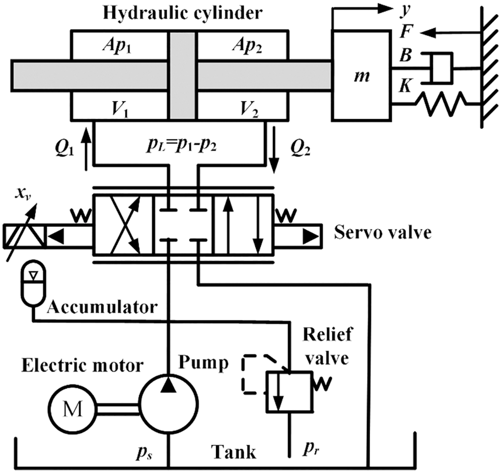
Figure 1: Schematic diagram of hydraulic servo system

Due to the fact that the dynamics of servo valve are much faster than the rest parts of system such that the dynamics can be neglected without loss of significance control performance. Thus, the dynamic equation of servo valve can be simplified as [36]

xv=ksvu (1)

where xv is the displacement of servo valve, ksv is the gain constant of servo valve, u is the control signal.

The flow rate of servo valve is controlled by the valve orifice. Regardless of the leakage, the load flow equation of servo valve is given as

QL=CdwxvPs−sign(u)PLρ (2)

where QL = (Q1 + Q2) is the real-time flow rates, where Q1 is the supply flow and Q2 is the return flow; Cd is the flow discharge coefficient; w is the area gradient of servo valve spool; ρ is the fluid oil mass density; Ps is the supply pressure; PL = P1 − P2 is the differential pressure of actuator, where P1 and P2 are the pressures in each side of the cylinder. The sign function represents the change in the direction of flow fluid through the servo valve, which is the main nonlinear factors.

According to the flow conservation law, the flow-pressure equation of hydraulic cylinder is described as follows

QL=Ay˙+CtPL+Vt4βeP˙L (3)

where A is the pressure area of the piston; y is the displacement of the cylindrical piston; Ct is the total leakage coefficient of the hydraulic actuator; Vt is the total volume of the actuator; βe is the effective bulk modulus of the hydraulic fluid.

The piston of hydraulic servo system can be modeled as the classical mass-spring-viscous system. According to Newton’s second law, the force balance equation of hydraulic actuator can be described by

APL=my¨+By˙+Ky (4)

where m is the mass of inertia load; K is the stiffness constant of spring; B is the damping coefficient of damper.

Define the system state variables x=[x1,x2,x3]T=[y,y˙,APL/m]T , then the state space representation of the hydraulic servo system can be formulated as

x˙1=x2x˙2=x3−Bmx2−Kmx1x˙3=4βeACdwksvmVtPs−sign(u)(mx3/A)ρu−4βeA2mVtx2−4βeCtVtx3 (5)

For hydraulic servo systems, the parameters Cd, ρ, K, B, βe and Ct are unknown positive constants. Considering nonlinear behaviors and modeling uncertainties, the state space model Eq. (5) can be rewritten as

x˙1=x2x˙2=x3+f¯2(x1,x2)+d2(x1,x2)x˙3=g¯3(x3,u)u+f¯3(x2,x3)+d3(x1,x2,x3) (6)

where f¯2(x1,x2)=−(B¯/m)x2−(K¯/m)x1 ; f¯3(x2,x3)=−(4β¯eA2/(mVt))x2−(4β¯eC¯t/Vt)x3 ; g¯3(x3,u)=(4β¯eAC¯dwksv/(mVtρ¯))Ps−sign(u)(mx3/A) , B¯,K¯,β¯e,C¯d,ρ¯,C¯t are nominal values of uncertain parameters respectively; d2(x1,x2) and d3(x1,x2,x3) are the lumped uncertain hydraulic parameters and unknown external loads respectively. d2 and d3 are bounded by |d2|≤d2max and |d3|≤d3max .

3  Controller Design

The control objective is to design a controller to let the x1 track the desired trajectory yd as closely as possible in the presence of nonlinear behaviors and modeling uncertainties.

3.1 Extend State Observer Design

Extend d2 as an additional state variable by defining xe1=d2 , and d3 as an additional state variable by defining xe2=d3 , then the state variable is extended to x=[x1, x2, xe1, x3, xe2] . Define h1(t) and h2(t) as the time derivative of xe1 and xe2 respectively. Then the system state representation can be rearranged as

x˙1=x2x˙2=x3+f¯2(x1,x2)+xe1x˙e1=h1(t)x˙3=g¯3(x3,u)u+f¯3(x2,x3)+xe2x˙e2=h2(t) (7)

The goal of the observer design is to estimate the lumped disturbances xe1 and xe2 for controller compensation in real time. Define x^ as the estimation of x and x~=x−x^ as the estimation error. From the extended system model Eq. (7), the extended state observers are constructed as

x^˙1=x^2+3ω1(x1−x^1)x^˙2=x^3+f¯2(x1,x2)+3ω12(x1−x^1)x^˙e1=ω13(x1−x^1)x^˙3=g¯3(x^3,u)u+f¯3(x2,x3)+2ω2(x1−x^1)x^˙e2=ω22(x1−x^1) (8)

where ω1>0 and ω2>0 are tunning parameters of the observer, which can be viewed as the bandwidths of the observer.

Combined with Eqs. (7) and (8), the dynamics of the state estimation errors can be written as

x~˙1=x~2−3ω1(x1−x^1)x~˙2=x~3+f~2(x1,x2)−3ω12(x1−x^1)x~˙e1=h1(t)−ω13(x1−x^1)x~˙3=g~3(x~3,u)u+f~3(x2,x3)−2ω2(x3−x^3)x~˙e2=h2(t)−ω22(x3−x^3) (9)

where f~2(x1,x2)=f2(x1,x2)−f2(x^1,x^2) , g~3(x~3,u)=g3(x3,u)−g3(x^3,u) , f~3(x2,x3)=f3(x2,x3)−f3(x^2,x^3) .

Define γ=[γ1,γ2,γ3]=[x~1,x~2/ωo1,x~e1/ωo12] , η=[η1,η2]=[x~3,x~e2/ωo2] , then Eq. (9) can be represented as

γ˙=ωo1A1γ+B1h1(t)ωo12η˙=ωo2A2γ+B2h2(t)ωo22 (10)

where

A1=[−3   1   0−3   0   1−1   0   0],B1=[001],A2=[−2   1−1   0],B2=[01] (11)

Note that A1 and A2 are Hurwitz, so there exists positive definite matrixes P11 and P12 satisfying the following equations

A1TP11+P11A1T=−I,A2TP22+P22A2T=−I (12)

Define a positive definite function Vo as

Vo=12γTP11γ+12ηTP22η (13)

The time derivative of Vo can be obtained as

V˙o=12[γ˙TP11γ+γTP11γ˙]+12[ηTP22η+ηTP22η]   =−12ωo1‖γ‖2+γTP11B1h1(t)ωo12−12ωo2‖η‖2 + ηTP22B2h2(t)ωo2 (14)

The upper bound of Eq. (14) can be achieved by

V˙o≤−12(ωo1−‖P11B1‖ωo14)‖γ‖2−12(ωo2−‖P22B2‖ωo22)‖η‖2+|h1|max2+|h2|max22 (15)

Define h0=(|h1|max2+|h2|max2)/2 , κ=min{ωo1−‖P11B1‖/ωo14,ωo2−‖P22B2‖/ωo22} , then the Eq. (15) can be rewritten as

V˙o≤−λV0+h0 (16)

where λ=0.5λmin{1,1/λmax(P11),1/λmax(P22)} .

Integrating Eq. (16), V˙o yields

Vo≤exp⁡(−λt)V0+h0λ[1−exp⁡(−λt)] (17)

According to Eq. (17), it can be indicated that state estimation and tracking error estimation are guaranteed to be bounded. Moreover, the extended state error can be regulated arbitrarily small by increasing the bandwidth tunning parameters.

3.2 Controller Design

Define sliding surface for each state variable

si=xi−αi−1 (18)

where i = 1,2,3, αi−1 is the estimation of xi , and si can converge to zero by the proper selection of αi−1 . In particular, α0=yd .

The sliding mode surface for the first subsystem is defined as s1=x1−yd , then

s˙1=x˙1−y˙d=x2−y˙d=s2+α1−y˙d (19)

Choose the virtual control item α1 as α1=−k1s1+y˙d . The Lyapunov function for the first subsystem is designed as

V1=12s12 (20)

where k1 is positive definite. Then the derivative of V1 can be derived as

V˙1=s1s˙1=s1(s2+α1−y˙d)=s1(s2−k1s1+y˙d−y˙d)=−k1s12+s1s2 (21)

The sliding mode surface for the second subsystem is defined as s2=x2−α1 , then the time derivative of s2 can be written as

s˙2=x˙2−α˙1 =x3+f¯2(x1,x2)+d2(x1,x2)−∂α1∂x1x˙1−∂α1∂ydyd(2)   =s3+α2+f¯2(x1,x2)−∂α1∂x1x2−∂α1∂ydyd(2)+d2(x1,x2) (22)

In order to make the second subsystem to reach the sliding mode surface, the virtual control item is defined as

α2=−k2s2−s1−f¯2(x1,x2)+∂α1∂x1x˙1+∂α1∂ydyd(2)−d2(x1,x2)μ2s2s22+ϵ22 (23)

where k2 is positive definite, μ2>1 and 0<ε2<1 are positive performance constants.

The Lyapunov function for the second subsystem is given by

V2=V1+12s22 (24)

Thus, the time derivative of V2 can be derived as

V˙2=V˙1+s2s˙2≤−k1s12+s1s2+s2s˙2 (25)

Substituting Eqs. (22) and (23) into Eq. (25)

V˙2≤−k1s12−k2s22+s2s3−d2(x1,x2)μ2s22s22+ε22+s2d2(x1,x2)   ≤−k1s12−k2s22+s2s3−|s2|d2(x1,x2)μ2|s2|s22+ε22+|s2|d2(x1,x2)   =−k1s12−k2s22+s2s3−|s2|d2(x1,x2)(μ2|s2|s22+ε22−1) (26)

To ensure the stability of the second subsystem, |s2|>ε2/μ22−1 . Then the Eq. (24) can be rewritten as

V˙2=V˙1+s2s˙2≤−k1s12−k2s22+s2s3 (27)

Similarly, the sliding mode surface for the third subsystem is defined as s3=x3−α2 , then the time derivative of s3 can be written as

s˙3=x˙3−α˙2 = g¯3(x3,u)+f¯3(x1,x2,x3)+d3(x1,x2.x3)−∑j=12∂α2∂xjx˙j−∑k=12∂α2∂yd(k)yd(k+1)  = g¯3(x3,u)+f¯3(x1,x2,x3)−∂α2∂x1x2−∂α2∂x2(x3+f¯2(x1,x2))−∂α2∂ydyd(2)−∂α2∂yd(2)yd(3)−∂α2∂x2d2(x1,x2)+d3(x1,x2.x3) (28)

Now, choosing the real control signal as

ub=1g¯3(x3,u)(−k3s3−s2−f¯3(x1,x2,x3)+∂α2∂x1x2+∂α2∂x2(x3+f¯2(x1,x2)))      +1g¯3(x3,u)(∂α2∂ydyd(2)+∂α2∂yd(2)yd(3)−(d3(x1,x2,x3)−∂α2∂x2d2(x1,x2))sgn(s3)) (29)

where k3 is positive definite. The candidate Lyapunov function for the third subsystem is given by

V3=V2+12s32 (30)

The first-order differential of the candidate Lyapunov function is given as

V˙3=V˙2+s3s˙3    ≤−k1s12−k2s22+s3s2+s3(−k3s3−s2−dΔ3sgn(s3)+d~Δ3)    ≤−k1s12−k2s22−k3s3−|s3|d¯Δ3+s3d~Δ3    ≤−k1s12−k2s22−k3s32 (31)

where dΔ3=∑j=12∂α2∂xjdj(x¯j)+d3(x¯3) , |dΔ3|≤d¯Δ3 , d¯Δ3 is a positive constant, d~Δ3=d¯Δ3−d^Δ3 .

According to Lyapunov theory, the dynamic system is globally asymptotically stable, which implies that the error will converge to zero even in the face of nonlinear behaviors and modeling uncertainties.

4  Simulation Results

The comparative simulations are conducted in MATLAB/Simulink software. The parameters of hydraulic system are selected as: m = 300 kg, Vt = 9 × 10−5m3, ρ = 900 kg/m3, A = 3.14 × 10−4m2, K = 1500 N/m, B = 1200 N·s/m, Ct = 4 × 10−3, ksv = 5.9 × 10−7 m/V, Cd = 0.62, βe = 6.9 × 108 Pa. In order to verify the effectiveness of the proposed controller, PID and backstepping controllers are tested for comparison. (1) PID: the control gains are set as Kp = 200, Ki = 80, Kd = 0.01, which is adjusted by a heuristic tunning method for small steady-state error and good transient response. (2) Backstepping: the constants are set as k1 = k2 = k3 = 2, μ2 = 1.5, ε2 = 0.6. (3) Presented controller: the bandwidths are set as ωo1=400 , ωo2=600 , the constants are set as k1 = k2 = k3 = 5, μ2 = 1.5, ε2 = 0.6. In particular, the parameters of these three controllers are well tuned with many times trial-and-error procedure to obtain satisfactory performance.

To simulate the nonlinear characteristics and external disturbances, the measurement noise of the displacement sensor and the input noise are 0.2% and 0.5% of the maximum ranges, respectively. The comparative tracking performance for sine motion with amplitude 10 mm and frequency 1 Hz is shown in Fig. 2. It can be seen that the presented controller can eliminate or attenuate the influence of lumped uncertainties better than the PID controller and backstepping controller. The tracking errors of different controllers are shown in Fig. 3. It is noted that the tracking errors of PID and backstepping have large chattering due to the lumped uncertainties and measurement noise. However, the presented controller achieves better disturbance compensation and smaller tracking error than the other two controllers. Specifically, the maximum trajectory error for PID and backstepping is 1.1 and 0.8 mm, respectively. The tracking error of presented controller is relatively very small, mostly within the 0.4 mm, which verifies the effectiveness of the presented control strategy.

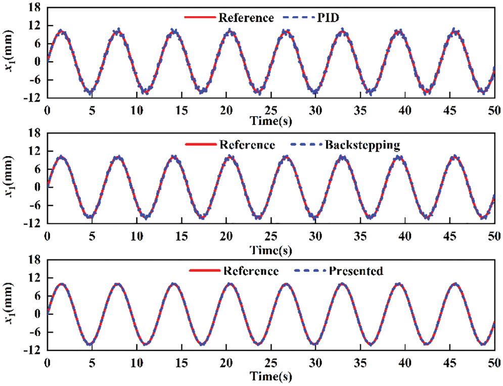
Figure 2: Comparative tracking performance for sine motion

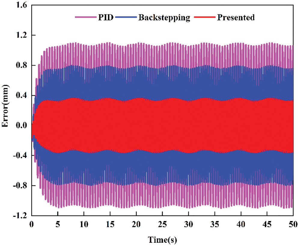
Figure 3: Comparative tracking errors for sine motion

Both the estimations xe1 and xe2 are shown in Fig. 4. The estimated states track the actual states quite well, which means that the observer has better tracking performance for the extend state although the system is subjected to external disturbance. Fig. 5 shows control input of three controllers. The proposed controller is free of chattering, which implies that it can successfully tackle the chattering problem and is easy to implement.

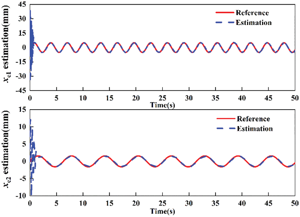
Figure 4: External disturbance estimation of presented controller

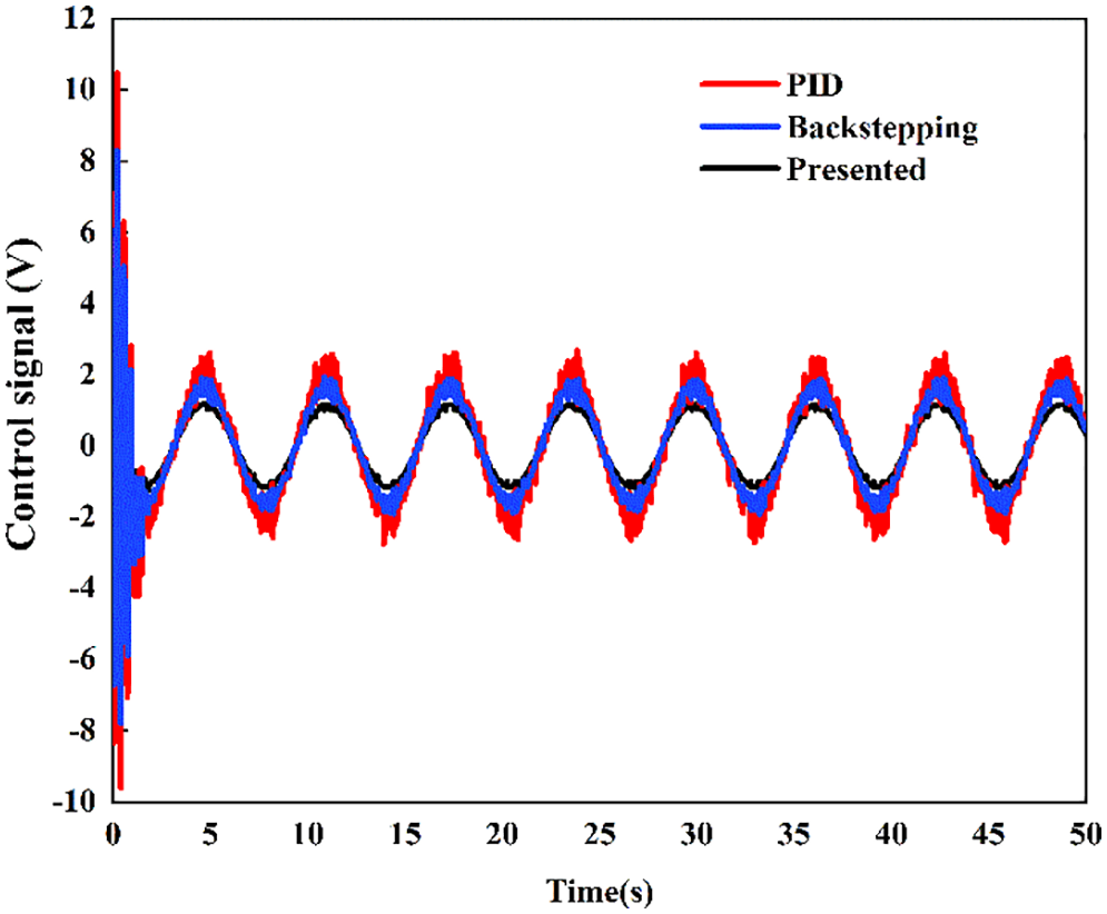
Figure 5: Control signal of presented controller

To quantitatively evaluate the tracking performance of different controllers, three error indices mean value of the absolute error, standard deviation of absolute error and integral of time multiplied by absolute error are defined as follows

{μ=1N∑i=1N|e1(i)|σ=1N∑i=1N(|e1(i)|−μ)2E=1N∑i=1NiTs|e1(i)| (32)

The performance indices of the different controllers are given in Table 1. For PID controller, the absolute error is about 0.6879 mm. For backstepping controller, the absolute error is reduced to 0.488 mm. For the presented controller, the absolute error is reduced to only 0.2156 mm. It can be seen that the proposed controller outperforms the other two controllers in terms of the other two performance indices, which means that the proposed control scheme is very helpful to alleviate the effects of nonlinear characteristics and external disturbance in hydraulic servo system.

5  Experiment Results

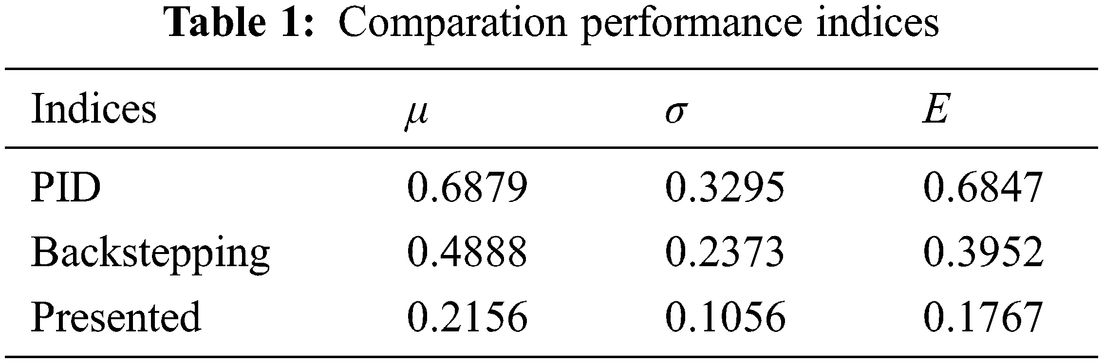
Fig. 6 shows the control scheme block diagram of hydraulic servo system. The host PC can monitor and send the command signal to the signal conditioner, where the control program is built by Matlab/Simulink. The DAC interface transforms digital signal into analogue signal. The power amplifier is used to enlarge the control signal and then drive the hydraulic actuator. The measured displacement and pressure signals acquired by sensors are sent to signal conditioner. The control objective of hydraulic servo system is to keep the actuator reproduce the desired signal as closely as possible. It should be noted that the parameters of the controller are consistent with those of simulation.

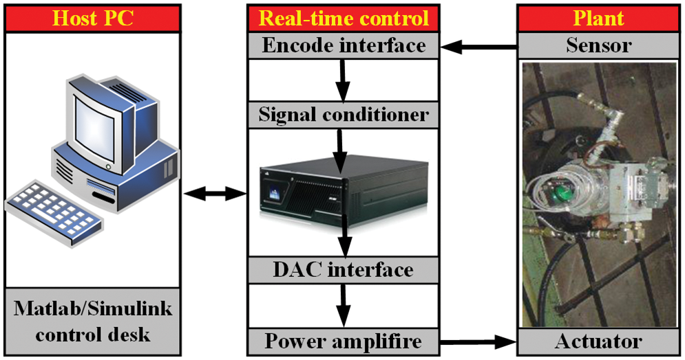
Figure 6: Control scheme block diagram of hydraulic servo system

The position comparative tracking performance for sine signal is given in Fig. 7 and their tracking errors are shown in Fig. 8. The experimental results show that the PID controller has maximum tracking error. The presented controller has a better tracking performance in terms of both disturbance compensation and error aspect than PID controller. Backstepping controller has an intermediate tracking error as compared to the presented controller and PID controller. Fig. 9 shows the control signal generated by controller, which is sent to servo valve of hydraulic system. When the PID controller is subjected to an external disturbance, a larger control signal is obviously produced. Whereas, the presented controller generates a low amplitude and fairly smooth control signal, which is critical to control system for energy minimization. The main reason why the proposed controller is more excellent compared with those controllers is that ESO is used to estimate lumped uncertainties and achieve active compensation.

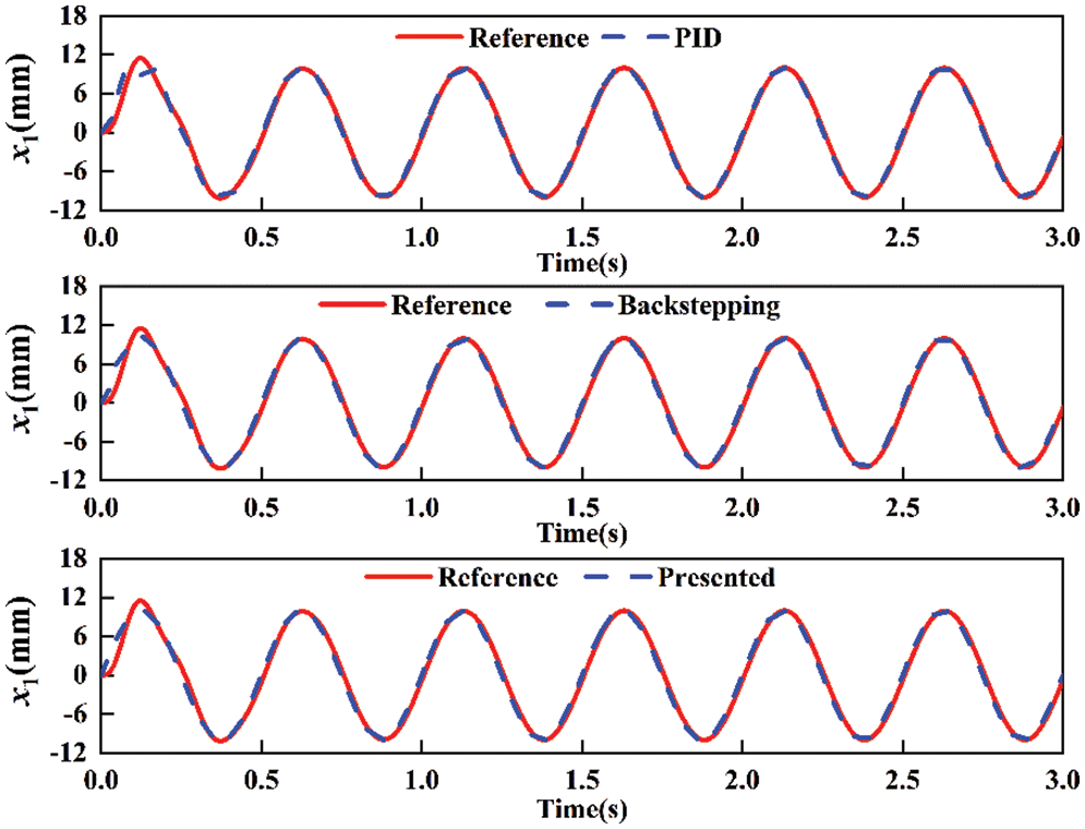
Figure 7: Comparative tracking performance for sine signal

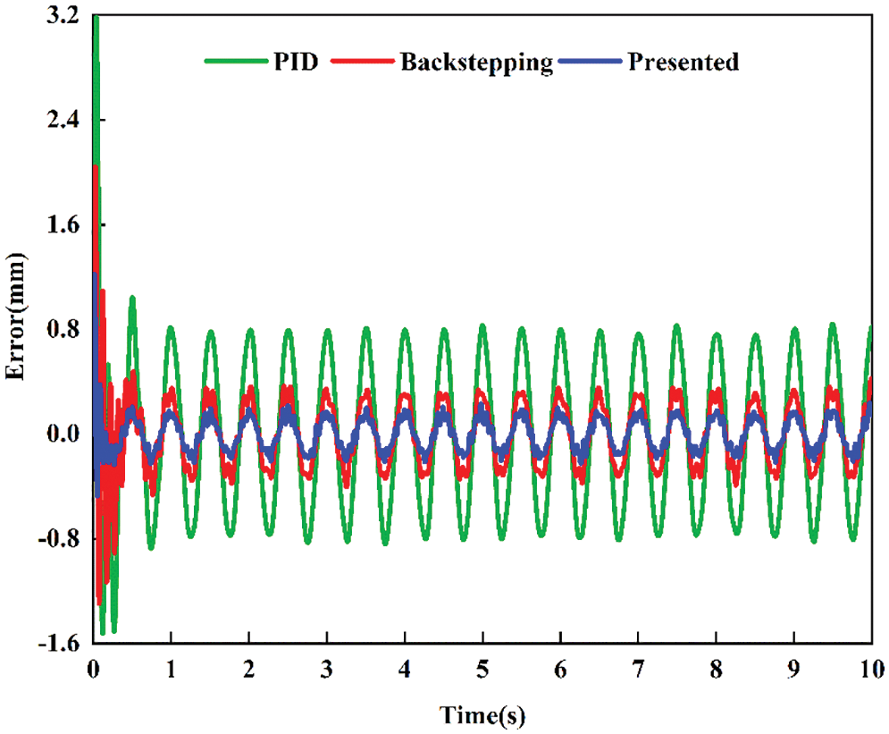
Figure 8: Comparative tracking error for sine signal

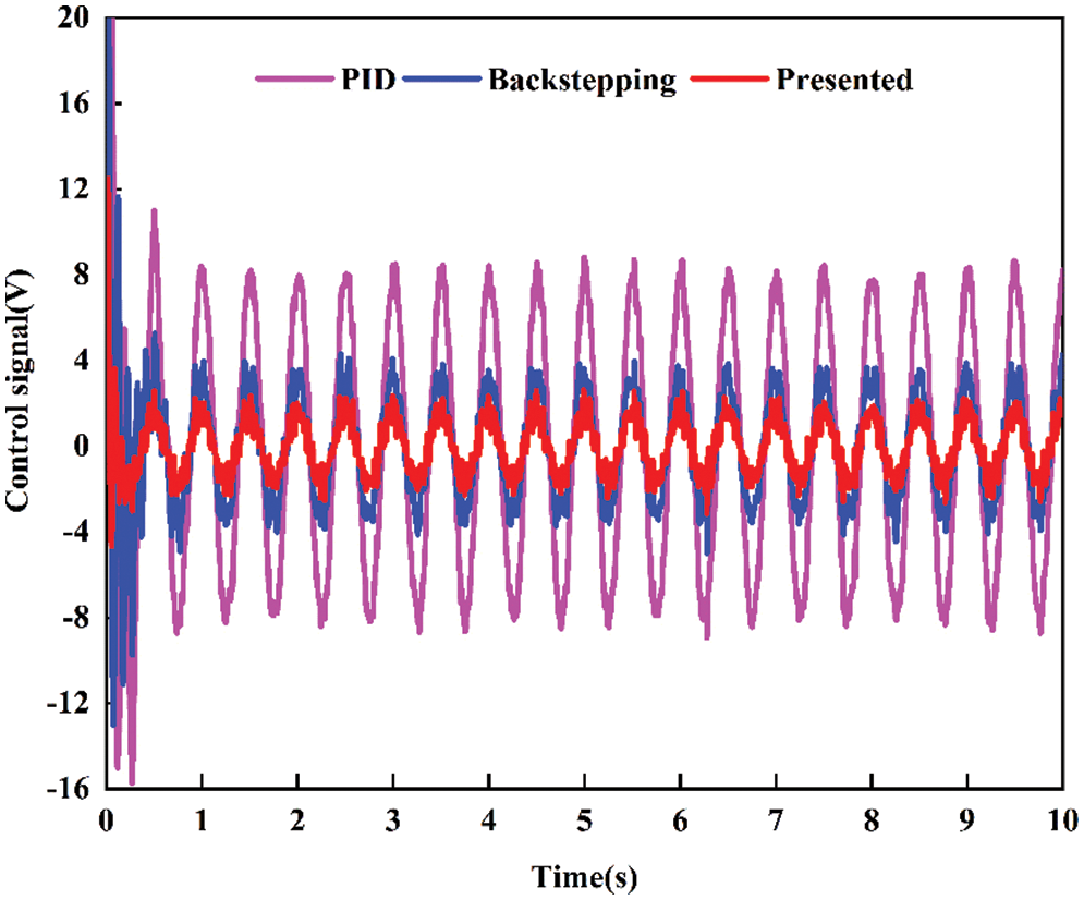
Figure 9: Comparative control signal for sine signal

The comparative tracking performance of the above controllers for square signal is shown in Fig. 10, and the tracking error curve is presented in Fig. 11. Obviously, the backstepping controller exhibits better performance than the PID controller. The maximum tracking error of backstepping is 0.6 mm; conversely, the PID controller has maximum error of 1 mm. However, the maximum position tracking error for the presented controller is only 0.4 mm.

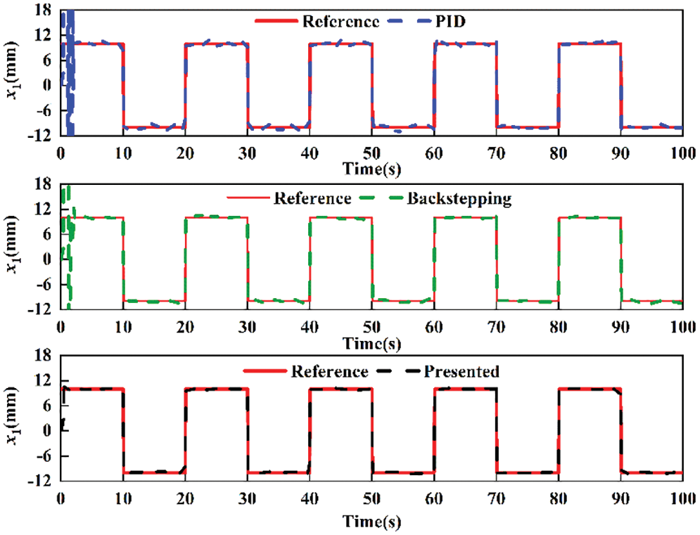
Figure 10: Comparative tracking performance for square signal

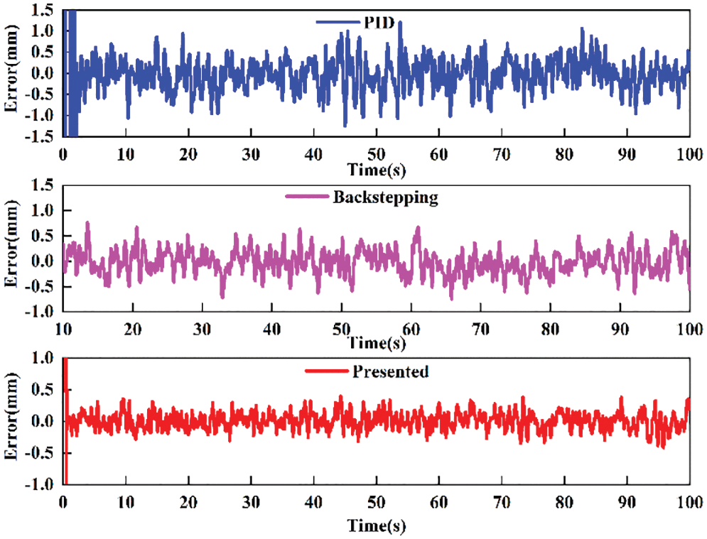
Figure 11: Comparative tracking error for square signal

The comparisons of position tracking and position tracking error for multi-frequency sine signal are shown in Figs. 12 and 13. The standard deviation of absolute error of PID, backstepping and proposed controllers is 0.3123, 0.1738 and 0.1351 mm, respectively. The results indicate that the proposed controller can track the desired signal well, while PID controller and backstepping controller do not realize good tracking performance.

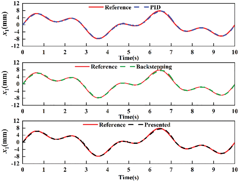
Figure 12: Comparative position tracking for multi-frequency sine signal

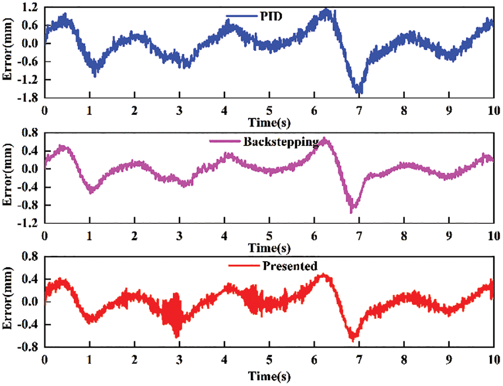
Figure 13: Comparative tracking error for multi-frequency sine signal

The concerned performance indices of different controllers for sine signal, square signal and multi-frequency sine signal are summarized in Fig. 14. For sine input signal, the μ of three controllers is about 0.5199, 0.2073 and 0.1047 mm. It is shown that the proposed controller outperforms the other two controllers again in terms of tracking precision. For square input signal, the σ of PID controller is about 0.2307 mm, the σ of backstepping controller is reduced to 0.1467 mm, the σ of presented controller is reduced to only 0.0826 mm. The smaller σ indicates the smoother tracking response, which is important for the steady-state performance of hydraulic servo system. For multi-frequency sine signal, the E of PID controller, backstepping controller and proposed controller is 0.3273, 0.1749 and 0.1438 mm, respectively. It is also found that the proposed method has the smallest three tracking errors and highest control precision. For three typical input signals, the proposed controller has better tracking performance than the other two controllers.

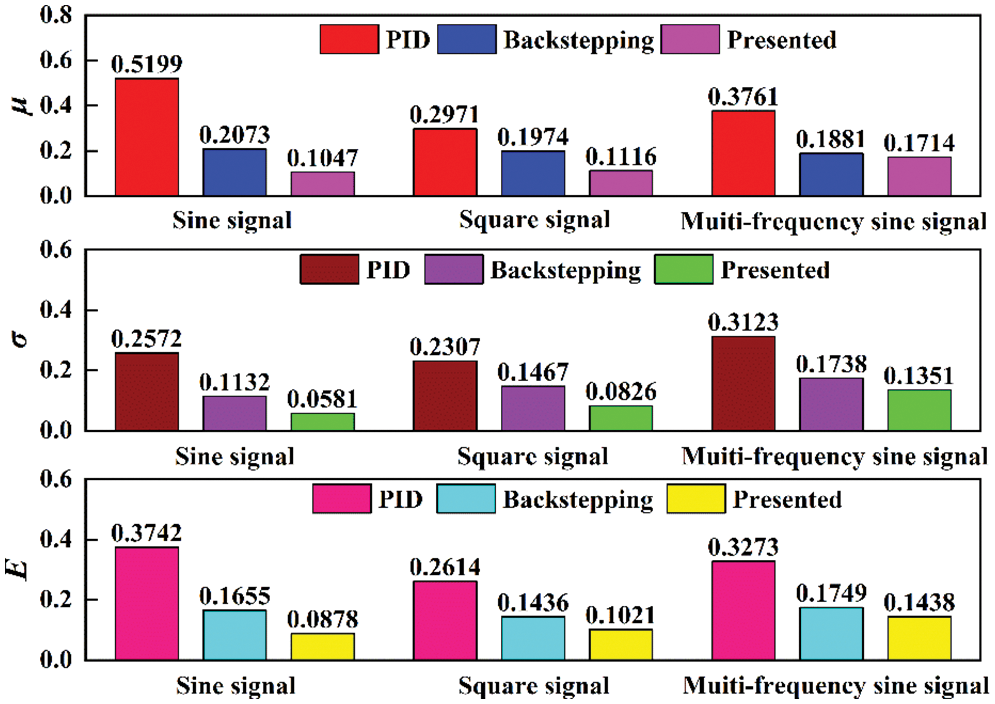
Figure 14: Comparation performance indices for different input signal

6  Conclusion

In this paper, a backstepping sliding mode control based on extended state observer is developed for the high precision tracking control of hydraulic servo system. The dynamic mathematical model of state space representation considering nonlinear characteristics and external disturbances is first constructed. Then, the extended state observation is introduced to estimate the lumped uncertainties. The controller is capable of forcing the position of the hydraulic servo system to track the desired trajectory in finite time and has robust behavior. The system stability is verified by Lyapunov criteria. Simulation and experimental comparative results validate the effectiveness of the proposed controller as compared to the PID controller and backstepping control.

Acknowledgement: The authors thank their families and colleagues for their continued support.

Funding Statement: The work is supported by the Key Science and Technology Program of Henan Province (Grant No. 222102220104), the Science and Technology Key Project Foundation of Henan Provincial Education Department (Grant No. 23A460014) and the High Level Talent Foundation of Henan University of Technology (Grant No. 2020BS043).

Conflicts of Interest: The authors declare that they have no conflicts of interest to report regarding the present study.

References

1. K. Guo, M. Li, W. Shi and Y. Pan, “Adaptive tracking control of hydraulic systems with improved parameter convergence,” IEEE Transactions on Industrial Electronics, vol. 69, no. 7, pp. 7140–7150, 2022. [Google Scholar]

2. X. W. Yang, W. X. Deng, J. Y. Yao and X. L. Liang, “Asymptotic adaptive tracking control and application to mechatronic systems,” Journal of the Franklin Institute-Engineering and Applied Mathematics, vol. 358, no. 12, pp. 6057–6073, 2021. [Google Scholar]

3. Z. L. Chen, Q. Guo, H. Y. Xiong, D. Jiang and Y. Yan, “Control and implementation of 2-DOF lower limb exoskeleton experiment platform,” Chinese Journal of Mechanical Engineering, vol. 34, no. 1, pp. 1–17, 2021. [Google Scholar]

4. Z. B. Xu, G. L. Qi, Q. Y. Liu and J. Y. Yao, “ESO-based adaptive full state constraint control of uncertain systems and its application to hydraulic servo systems,” Mechanical Systems and Signal Processing, vol. 167, no. 3, pp. 108560, 2022. [Google Scholar]

5. Y. Tang, Z. C. Zhu, G. Shen, G. C. Rui, D. Cheng et al., “Real-time nonlinear adaptive force tracking control strategy for electrohydraulic systems with suppression of external vibration disturbance,” Journal of the Brazilian Society of Mechanical Sciences and Engineering, vol. 41, no. 7, pp. 278, 2019. [Google Scholar]

6. J. S. Zhao, G. Shen, C. F. Yang, W. D. Zhu and J. Y. Yao, “A robust force feed-forward observer for an electro-hydraulic control loading system in flight simulators,” ISA Transactions, vol. 89, no. 1, pp. 198–217, 2019. [Google Scholar] [PubMed]

7. G. Palli, S. Strano and M. Terzo, “Sliding-mode observers for state and disturbance estimation in electro-hydraulic systems,” Control Engineering Practice, vol. 74, no. 9, pp. 58–70, 2018. [Google Scholar]

8. W. C. Sun, H. J. Gao and B. Yao, “Adaptive robust vibration control of full-car active suspensions with electrohydraulic actuators,” IEEE Transactions on Control Systems Technology, vol. 21, no. 6, pp. 2417–2422, 2013. [Google Scholar]

9. X. Li, Z. C. Zhu and G. Shen, “A switching-type controller for wire rope tension coordination of electro-hydraulic-controlled double-rope winding hoisting systems,” Proceedings of the Institution of Mechanical Engineers Part I-Journal of Systems and Control Engineering, vol. 230, no. 10, pp. 1126–1144, 2016. [Google Scholar]

10. M. Fallahi, M. Zareinejad, K. Baghestan, A. Tivay, S. M. Rezaei et al., “Precise position control of an electro-hydraulic servo system via robust linear approximation,” ISA Transactions, vol. 80, no. 11, pp. 503–512, 2018. [Google Scholar] [PubMed]

11. D. Won, W. Kim and M. Tomizuka, “High-gain-observer-based integral sliding mode control for position tracking of electrohydraulic servo systems,” IEEE-ASME Transactions on Mechatronics, vol. 22, no. 6, pp. 2695–2704, 2017. [Google Scholar]

12. J. Park, B. Lee, S. Kang, P. Y. Kim and H. J. Kim, “Online learning control of hydraulic excavators based on echo-state networks,” IEEE Transactions on Automation Science and Engineering, vol. 14, no. 1, pp. 249–259, 2017. [Google Scholar]

13. M. E. M. Essa, M. A. S. Aboelela, M. A. M. Hassan and S. M. Abdrabbo, “Model predictive force control of hardware implementation for electro-hydraulic servo system,” Transactions of the Institute of Measurement and Control, vol. 41, no. 5, pp. 1435–1446, 2019. [Google Scholar]

14. G. Wrat, M. Bhola, P. Ranjan, S. K. Mishra and J. Das, “Energy saving and fuzzy-PID position control of electro-hydraulic system by leakage compensation through proportional flow control valve,” ISA Transactions, vol. 101, no. 5, pp. 269–280, 2020. [Google Scholar] [PubMed]

15. S. Chen, Z. Chen, B. Yao, X. C. Zhu, S. Q. Zhu et al., “Adaptive robust cascade force control of 1-DOF hydraulic exoskeleton for human performance augmentation,” IEEE-ASME Transactions on Mechatronics, vol. 22, no. 2, pp. 589–600, 2017. [Google Scholar]

16. T. A. Davis, Y. C. Shin and B. Yao, “Adaptive robust control of machining force and contour error with tool deflection using global task coordinate frame,” Proceedings of the Institution of Mechanical Engineers Part B-Journal of Engineering Manufacture, vol. 232, no. 1, pp. 40–50, 2018. [Google Scholar]

17. C. Cheng, S. Y. Liu and H. Z. Wu, “Sliding mode observer-based fractional-order proportional-integral-derivative sliding mode control for electro-hydraulic servo systems,” Proceedings of the Institution of Mechanical Engineers Part C-Journal of Mechanical Engineering Science, vol. 234, no. 10, pp. 1887–1898, 2020. [Google Scholar]

18. W. M. Bessa, M. S. Dutra and E. Kreuzer, “Sliding mode control with adaptive fuzzy dead-zone compensation of an electro-hydraulic servo-system,” Journal of Intelligent and Robotic Systems, vol. 58, no. 4, pp. 3–16, 2010. [Google Scholar]

19. Q. Guo, Y. Zhang, B. G. Celler and S. W. Su, “Backstepping control of electro-hydraulic system based on extended-state-observer with plant dynamics largely unknown,” IEEE Transactions on Industrial Electronics, vol. 63, no. 11, pp. 6909–6920, 2016. [Google Scholar]

20. G. P. Liu and S. Daley, “Optimal-tuning PID controller design in the frequency domain with application to a rotary hydraulic system,” Control Engineering Practice, vol. 8, no. 9, pp. 1045–1053, 2000. [Google Scholar]

21. Z. Chen, F. H. Huang, C. N. Yang and B. Yao, “Adaptive fuzzy backstepping control for stable nonlinear bilateral teleoperation manipulators with enhanced transparency performance,” IEEE Transactions on Industrial Electronics, vol. 67, no. 1, pp. 746–756, 2020. [Google Scholar]

22. J. Jiang, J. Guo, B. Yao and Q. W. Chen, “Adaptive robust control of mobile satellite communication system with disturbance and model uncertainties,” Journal of Systems Engineering and Electronics, vol. 23, no. 5, pp. 761–767, 2012. [Google Scholar]

23. Z. B. Xu, D. W. Ma, J. Y. Yao and N. Ullah, “Feedback nonlinear robust control for hydraulic system with disturbance compensation,” Proceedings of the Institution of Mechanical Engineers Part I-Journal of Systems and Control Engineering, vol. 230, no. 9, pp. 978–987, 2016. [Google Scholar]

24. T. Gao, Y. J. Liu, L. Liu and D. Li, “Adaptive neural network-based control for a class of nonlinear pure-feedback systems with time-varying full state constraints,” IEEE-CAA Journal of Automatica Sinica, vol. 5, no. 5, pp. 923–933, 2018. [Google Scholar]

25. Y. J. Liu, Q. Zeng, L. Liu and S. C. Tong, “An adaptive neural network controller for active suspension systems with hydraulic actuator,” IEEE Transactions on Systems Man Cybernetics-Systems, vol. 50, no. 12, pp. 5351–5360, 2020. [Google Scholar]

26. Z. K. Yao, Y. P. Yu and J. Y. Yao, “Artificial neural network-based internal leakage fault detection for hydraulic actuators: An experimental investigation,” Proceedings of the Institution of Mechanical Engineers Part I-Journal of Systems and Control Engineering, vol. 232, no. 4, pp. 369–382, 2018. [Google Scholar]

27. Z. H. U. Dachang, “Sliding mode synchronous control for fixture clamps system driven by hydraulic servo systems,” Proceedings of the Institution of Mechanical Engineers Part C-Journal of Mechanical Engineering Science, vol. 221, no. 9, pp. 1039–1045, 2007. [Google Scholar]

28. K. Shao, J. C. Zheng, K. Huang, H. Wang, Z. H. Man et al., “Finite-time control of a linear motor positioner using adaptive recursive terminal sliding mode,” IEEE Transactions on Industrial Electronics, vol. 67, no. 8, pp. 6659–6668, 2020. [Google Scholar]

29. J. Y. Yao, W. X. Deng and Z. X. Jiao, “RISE-based adaptive control of hydraulic systems with asymptotic tracking,” IEEE Transactions on Automation Science and Engineering, vol. 14, no. 3, pp. 1524–1531, 2017. [Google Scholar]

30. K. Shao, J. H. Zheng, H. Wang, X. Q. Wang and B. Liang, “Leakage-type adaptive state and disturbance observers for uncertain nonlinear sytems,” Nonlinear Dynamics, vol. 105, no. 3, pp. 2299–2311, 2021. [Google Scholar]

31. J. Y. Yao, Z. X. Jiao and B. Yao, “Robust control for static loading of electro-hydraulic load simulator with friction compensation,” Chinese Journal of Aeronautics, vol. 25, no. 6, pp. 954–962, 2012. [Google Scholar]

32. Q. Guo, Y. L. Liu, D. Jiang, Q. Wang, W. Y. Xiong et al., “Prescribed performance constraint regulation of electrohydraulic control based on backstepping with dynamic surface,” Applied Sciences-Basel, vol. 8, no. 1, pp. 76, 2018. [Google Scholar]

33. M. J. Li, J. H. Wei, J. H. Fang, W. Z. Shi and K. Guo, “Fuzzy impedance control of an electro-hydraulic actuator with an extended disturbance observer,” Frontiers of Information Technology & Electronic Engineering, vol. 20, no. 9, pp. 1221–1233, 2019. [Google Scholar]

34. G. Yang, J. Y. Yao and Z. Dong, “Neuroadaptive learning algorithm for constrained nonlinear systems with disturbance rejection,” International Journal of Robust and Nonlinear Control, vol. 32, no. 10, pp. 6127–6147, 2022. [Google Scholar]

35. S. Wang, H. Yu, J. Yu, J. Na and X. Ren, “Neural-network-based adaptive funnel control for servo mechanisms with unknown dead-zone,” IEEE Transactions on Cybernetics, vol. 50, no. 4, pp. 1383–1394, 2020. [Google Scholar] [PubMed]

36. G. Shen, Z. C. Zhu, J. S. Zhao, W. D. Zhu, Y. Tang et al., “Real-time tracking control of electro-hydraulic force servo systems using offline feedback control and adaptive control,” ISA Transactions, vol. 67, no. 2, pp. 356–370, 2017. [Google Scholar] [PubMed]