Simulated Annealing with Deep Learning Based Tongue Image Analysis for Heart Disease Diagnosis

1  Introduction

Coronary heart disease (CHD) has become a crucial part of cardiovascular disease (CVD) and the leading factor which causes death and disability across the world. CHD is considered a major health issue which burdens medical treatment and society [1]. Improving the prevention level and treatment of CHD is highly significant because of the rising mortality of CHD in China [1]. Current research on TCM syndromes of CHD display that phlegm and blood stasis syndrome (PBSS) accounts for a rising percentage of CHD syndromes [1,2]. The most dominant disease of Traditional Chinese Medicine (TCM) is CHD, accumulating 2,000 years of treatment practice [2]. TCM contains unique benefits in CHD treatment and displays favourable efficiency. The worldwide demand for basic healthcare assistance and technology development allows the platforms for point-of-care (POC) diagnostics [3]. Despite the current advancements in automatic disease diagnosing tools, the requirement of blood serum through recognition time, inexperience, reliability, precision, and the need for a second confirmatory test were the problems that must be overtaken. Therefore, skin color, temperature, retinopathy, facial expressions, tongue diagnosis, and surface are vital variables for future smartphone-oriented clinical expert systems for attaining non-invasiveness, simplicity, automatic analysis, and immediacy [4].

Tongue diagnosis becomes an effectual non-invasive process to measure the inner organ condition of the patient. The diagnosis procedure is reliable based on experts’ opinions on visual inspection encompassing the tongue’s form, color, coating, motion, and substance [5]. Conventional tongue diagnosis was inclined to identify the syndrome instead of the abnormal appearance and disease of the tongue [6]. For example, the tongue coating’s yellow-dense and white-greasy appearance specify hot and cold syndromes, which can be linked with health conditions like endocrine disorders or immune, infection, stress, and inflammation, which can be 2 parallel but correlated syndromes from TCM. Abolishing the dependence on the subjective and experience-related valuation of tongue analysis might raise the scope for broader usage of tongue diagnosis globally, including in Western medicine [7]. Computerized tongue examination containing geometry study, color correction, image investigation, tongue segmentation, light estimation, etc., is a potential tool for diagnosing disease targeting to overcome such concerns.

The benefit of tongue diagnosis, it is a non-invasive and simple method. But it becomes hard to gain a standardized and objective examination. Variations in inspection conditions, like light sources, influence outcomes significantly [8]. Furthermore, because the diagnosis depends on the knowledge and experience of the clinician, it becomes difficult to gain a standardized outcome. Currently, several research works are being conducted to solve such issues. This study summarises the advancement of current technologies and tongue diagnosis [9]. The general computerized tongue diagnosis procedure is classified into 2 methods. Firstly, the conventional machine learning (ML) technique. This technique generally segregates the raw tongue image, extracts features like shape, color, spectrum, and texture from the tongue image segmented and chooses the classifier to attain tasks like recognition and classification at the end [10]. Secondly, the deep learning (DL) technique generally utilizes raw data for feature extraction and training by convolution functions.

This manuscript introduces a novel Simulated Annealing with Transfer Learning based Tongue Image Analysis for Disease Diagnosis (SADTL-TIADD) model. The presented SADTL-TIADD model focuses on detecting and classifying diseases using tongue images, namely CVD and pneumonia. To accomplish this, the SADTL-TIADD model was initially Bilateral Filter (BF) based pre-processing and CLAHE-based contrast enhancement. Next, the presented SADTL-TIADD technique employed an EfficientNet-based feature extractor to generate useful feature vectors. The SA with the extreme learning machine (ELM) model enhances classification efficiency for disease detection and classification. To ensure the improved performance of the SADTL-TIADD system, a wide-ranging set of simulations can be performed.

2  Related Works

The author in [11] utilises deep transfer learning (DTL) to analyse tongue images. First, tongue features are extracted using the pre-trained networks (Inception_v3 and ResNet), and later modification of the resultant layer of the original network with fully connected (FC) and global average pooling layers to output classification result. In [12], a lightweight segmentation method for tongue images is developed under the elementary encoding-decoding architecture. MobileNet v2 is accepted as the backbone network because of its lower computational complexity and fewer parameters. The lower-level positional and higher-level semantic data are combined to identify the tongue-body boundary. Then, the dilated convolutional operation is implemented on the last feature map of networks to expand the receptive field, capturing rich global semantic data.

In [13], the authors presented a Chinese Medicine based diabetes diagnosis dependent upon examining the extracting feature of the panoramic tongue image, namely texture, colour, shape, fur, and tooth markings. The extracting feature can be performed using Convolutional Neural Network (CNN)—ResNet50 model, and the classifier can be done using the presented Deep RBFNN approach based on an autoencoder (AE) learning module. Zhou et al. [14] developed an end-to-end mechanism for multi-task learning of tongue segmentation and localization, termed TongueNet, where pixel-level previous data is exploited for supervised training Deep CNN (DCNN). A feature pyramid network (FPN) is primarily introduced based on the context-aware residual block for extracting multiscale tongue features. Next, the tongue candidate’s region of interest (ROI) is positioned in the extracting feature map. Lastly, finer segmentation and localization of the tongue body were carried out based on the feature map of ROI.

In [15], the authors developed a computer-aided intelligent decision support mechanism. The CNN and DenseNet architecture was applied to identify the tongue images’ essential features, namely the fur coating, colour, texture, red spots, and tooth markings. The classifier support vector machine (SVM) has been applied to enhance the accuracy of the SVM parameter is tuned using the PSO algorithm. The authors in [16] proposed a 2-stage methodology dependent upon tongue landmarks and tongue region recognition through DL. Initially, a cascaded CNN is introduced for simultaneously detecting the tongue region and tongue landmark to maximize discriminatory data and minimize the redundancy data explicitly. Next, the identified region and landmark of the tongue are sent to a fine-grained classifier system for the last detection.

Wang et al. [17], an AI architecture with DCNN for detecting the tooth-marked tongue. Firstly, a larger dataset with 1548 tongue images is applied. Next, ResNet34 CNN infrastructure is used for extracting features and implementing classifiers. Mansour et al. [18] designed an automatic IoT and synergic DL-based tongue colour image (ASDL-TCI) investigation mechanism to classify and diagnose diseases. Initially, we used the IoT device to capture the human tongue image and transferred it to the cloud for detailed examination. Moreover, SDL-based feature extraction techniques and median filtering (MF) based image pre-processed is executed. In addition, DNN-based classification was employed to define the presence of diseases. Finally, enhanced black widow optimization (EBWO) based parameter tuning is performed to improve the detection accuracy. Though several ML and DL models for tongue image analysis are available in the literature, it is still needed to enhance the classification performance. Owing to the continual deepening of the model, the number of parameters of ML and DL models also increases quickly, which results in model overfitting. Since the trial and error method for parameter tuning is tedious and erroneous, metaheuristic algorithms can be applied. Therefore, in this work, we employ the SA algorithm for the parameter selection of the ELM model.

3  The Proposed Model

This study introduced a novel SADTL-TIADD approach to detect and classify diseases utilizing tongue images. To accomplish this, the SADTL-TIADD approach initially BF-based pre-processing and CLAHE-based contrast enhancement. Next, the presented SADTL-TIADD technique employed an EfficientNet-based feature extractor to generate useful feature vectors. For disease detection and classification, the SA with the ELM model is applied, and using SA enhances the classification efficiency. Fig. 1 depicts the block diagram of the SADTL-TIADD approach.

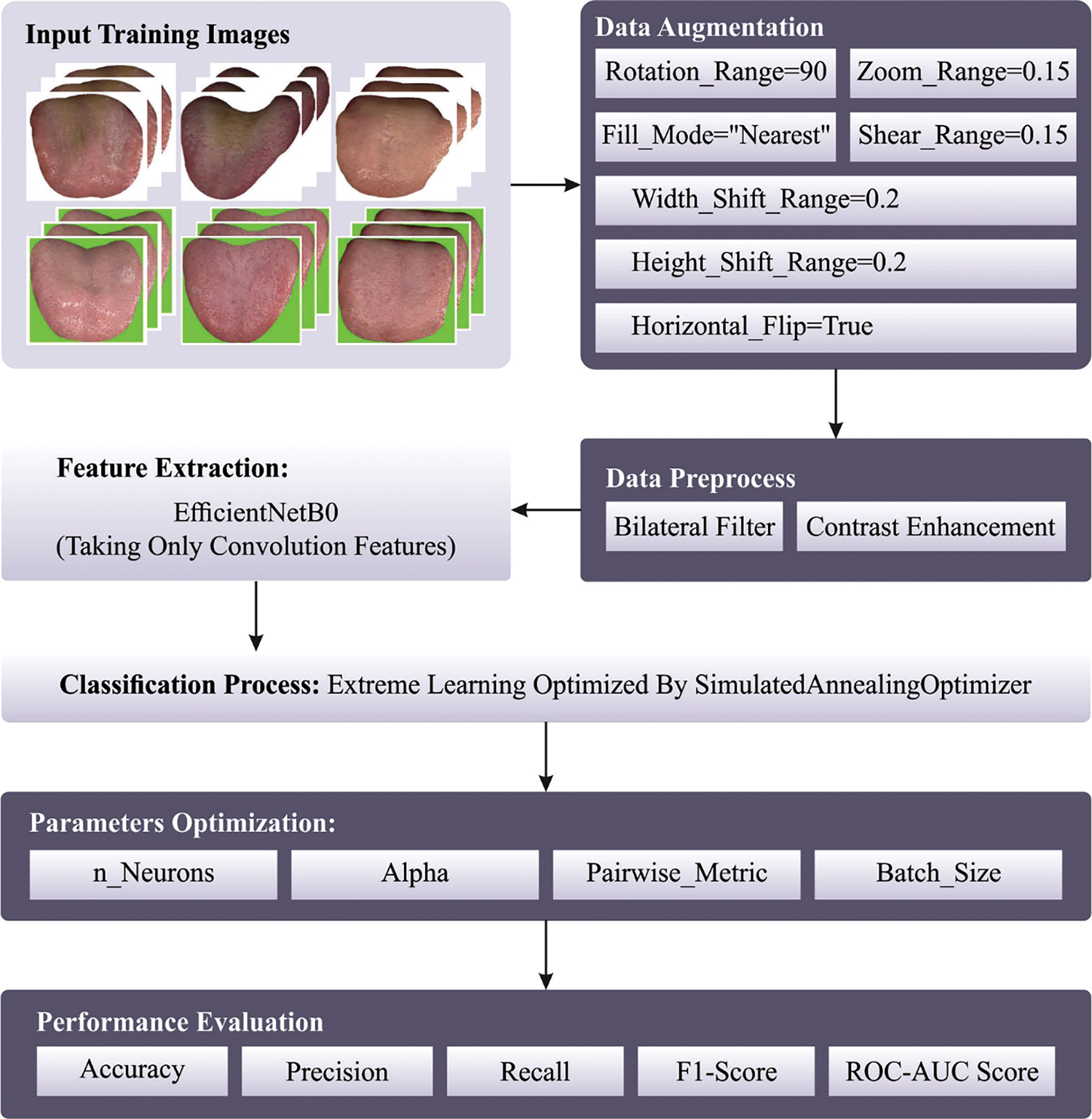
Figure 1: Block diagram of SADTL-TIADD approach

3.1 Image Pre-Processing

Primarily, the SADTL-TIADD model follows BF-based pre-processing and CLAHE-based contrast enhancement. Consider the BF employed to a 2D grayscale image x. Where p∈Z2 shows the location of the objective pixel and xp∈R1 denotes their pixel intensity, and q∈𝒩p represents an adjacent pixel of p, let 𝒩p⊂Z2 be the set of adjacent pixels at p, viz., a rectangular domain reinforced in a filter window [19]:

BF(p):=∑qϵNpws(p,q)⋅wr(gp,gq)⋅xq∑qϵNpws(p,q)⋅wr(gp,gq).(1)

In Eq. (1), gp refers to the objective pixel in a guide image, and gq is among their adjacent pixels. The description is similar to the original BF once it can be self-guided, i.e., gp=xp and gq=xq.

The previous weight ws(p,q) demonstrated the location of the pixel region was represented as the spatial kernel. The last weight wr(GP,gq), which represents the pixel domain's intensity, was denoted as the range kernel. They set as even-symmetric unimodal operation, for instance, a Lorentzian or Gaussian function:

ws(p,q):=exp⁡(−12σs2‖p−q‖22),(2)

wr(gp,gq):=exp⁡(−12σr2(gp−gq)2)

The BF smooths an objective image using the adjacent pixel with the same intensity value that the objective pixel xp, as demonstrated in Eq. (1). This process might prevent smoothing edges equivalent to individuals of guide images since the colours or intensities nearby the edge region changes dramatically. CLAHE is a type of Adaptive Histogram Equalization (AHE) technique [20]. The CLAHE resolves the over-amplification problems of traditional AHE through the number of tiles parameters and the clip limit. CLAHE splits the image as MxN local tiles. For all the tiles, the histogram has been separately calculated. The histogram first evaluates each region's average number of pixels for computers.

NA=NX×NYNG(3)

Here, Na represents the average count of pixels, Nx indicates the count of pixels from the X dimensional, NY shows the count of pixels from theY dimensional, and NG shows the number of gray levels. Next, determine the clip limit from Eq. (4) for clipping the histogram.

NCL=NA×NNCL(4)

In the following, NCL denotes the clip limit, and NNCL shows the normalization clip limit between zero and one. Then, for all the tiles, the clip limit was employed for the height of the histogram.

Hi={NCLif Ni≥NCLNielsei=1,2,…,1−1(5)

Let, Hi be the height of the histogram of i-th tiles, Ni shows the histogram of i-th tiles, and L indicates the number of grey levels. The overall number of clipped pixels is calculated as follows.

Nc=(NX×NY)−∑i=0L−1Hi(6)

where NC indicates the count of clipped pixels. After computing NC, redistribute the clipped pixel. The pixel is redistributed uniformly/non-uniformly. Calculating the count of pixels that redistribute is as follows.

NR=NCL(7)

where NR denotes the count of pixels that redistribute. Afterwards, the clipped histogram was normalized as follows.

Hi={NCLif Ni+NR≥NCLNi+NRelsei=1,2,…,1−1(8)

Eqs. (6) and (7) compute the number of un-distributed pixels. Eq. (8) is repeated until each pixel is redistributed. At last, the cumulative histogram of the context region is formulated as follows.

Ci=1(NX×NY)∑j=0iHj(9)

Afterwards, the calculation was done, and the histogram of context region corresponded with uniform, Rayleigh, or exponential possibility distribution that provides an attached brightness and visual quality. The pixel P(X,Y) with the value of s and 4 centre points belongs to the neighbouring tiles as R1, R2, R3, and R4. The weight sums are calculated over these 4 context regions. To the resultant image, tiles are combined, and the bilinear interpolation completes the removal of artefacts amongst the independent tiles; the novel value of s can be represented by s′ is attained by the following expression.

s′=(1−y)((1−X)×R1(s)+X×R2(s))+y((1−X)×R3(s)+X×R4(s)))(10)

Lastly, the enhanced image is attained.

3.2 Feature Extraction

At this stage, the presented SADTL-TIADD technique employed an EfficientNet-based feature extractor to generate useful feature vectors. The EfficientNet-B0 network exploits the recombination coefficient to automatically adjust the model's resolution, depth, and width and has features of high recognition accuracy and small parameters [21]. The input of EfficientNet-B0 is RGB (Red, blue, green) three-channel oil tea image with 224×224 pixel resolution, involving 2 convolution layers, 16 Mobile Inverted Bottleneck Convolution (MBConv) modules, 1 classification layer, and 1 global average pooling layer. MB Conv uses a drop connect rather than a conventional dropout, which plays a major role in preventing the model from overfitting.

EfficientNet-B0 scaling tries to extend the resolution (Hi,Wi), length (Li), and width (Ci) of the network without changing Fj predetermined in the baseline network and restrict the uniform scaling of each layer at a constant ratio to decrease the design space. To obtain the maximum model accuracy under any given resource constraints, the target is expressed through the following optimization problem:

maxd,w,rAccuracy(N(d,w,r))

s.t.N(d,w,r)=⨀i=1,…sF^id⋅L^i(X⟨r⋅Hi,^r⋅Wi^w⋅C^i})(11)

Memory (N)≤tar−memory

Flops(N)≤tar−flops

In Eq. (11), w and r denote the scaling network’s depth, width, and resolution coefficients. Furthermore, F^i,Li^, and C^i refer to the predetermined network architecture, predetermined layers, and channels correspondingly, and Hi^ and Wi^ denotes predetermined resolutions. Furthermore, <H^i,w^i, C^j> signifies the shape of input tensor X corresponding to layer i, Memory (N) and Flops (N) are the parameters and floating point of the network operation, correspondingly. Lastly, tar-flops and tar-memory are floating points of the operation and the threshold of the parameter correspondingly.

In EfficientNet-B0, the compound coefficient φ is used for uniformly scaling the resolution, depth, and width of the network to obtain better accuracy and efficiency and balance the relationships between the three dimensions in the following:

d=αϕ,w=βϕ,r=γϕ

s.t.  α⋅β2⋅γ2≈2(12)

α≥1,β≥1,γ≥1

Let ϕ be a user-defined coefficient controlled based on available resources. Instinctively, β and γ represent the resource control coefficient that determines how to correspondingly assign the resource to the resolution, depth, and width.

3.3 Image Classification

For disease detection and classification, the SA with the ELM model enhances classification efficiency. ELM is an ML system that depends on an FFNN with an individual layer [22]. In ELM, computing the hidden state parameter is the method to determine the output weight, and the hidden state is stochastically constructed. This architecture approaches have a fast convergence rate and low computation difficulty. Also, it has benefits in generalization performance and fitting ability that of conventional gradient-based learning model. The typical ELM three-layer architecture has been demonstrated in Fig. 2.

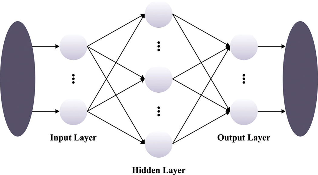
Figure 2: ELM structure

The complete overview of the ELM traffic flow forecasting method is shown in the following. Firstly, the traffic flow at a measurement position at the i-th time interval is represented by μi(a). Next, we employed {(e(i),t(i))}i=1N for demonstrating N traffic flow training instances. Then, the traffic flow at the historical and existing ν−1 time interval is fixed to e(i)=[μi−ν+1(a),…,μi(a)]a=1A, while A indicates the number of measurement positions and ν indicates the time lag. Then, the factual dataset of the i specimen for the traffic flow predictive method is characterized as f(i)=[μi+1(a)]a=1A. The FFNN with a w0 hidden nodes are shown below:

Hβ=T,(13)

Now H=(gij)i=1,…N,j=1,…w0 designates the output matrix of hidden state. Amongst them, gij=f(χjTei+ωj) means the resultant of jth hidden nodes concerning ei. The input node and j-th hidden neurons are connected through a weighted vector χj= [χj1,χj2,…,χjn]T. ωj signifies the bias of jth hidden neurons. The matrix of output weight is stated as β=[β1,β2,…,βw0]T, and connected the output node and the equivalent jth hidden neurons through the weighted vector j=1, …, w0. The objective matrix is signified by T=[t1,t2,…,tN]T. The functioning method of ELM is to modify the input weight and hidden deviance randomly. Next, a rational activation function is selected for ascertaining the matrix H. Then, by estimating the linear scheme’s least square (LS) solution that performs a role in FFNN training, the output weight ψ is evaluated as follows.

β^=H†T,(14)

Here H† signifies the Moore-Penrose (MP) generalized inverse of matrix H.

3.4 Hyperparameter Tuning

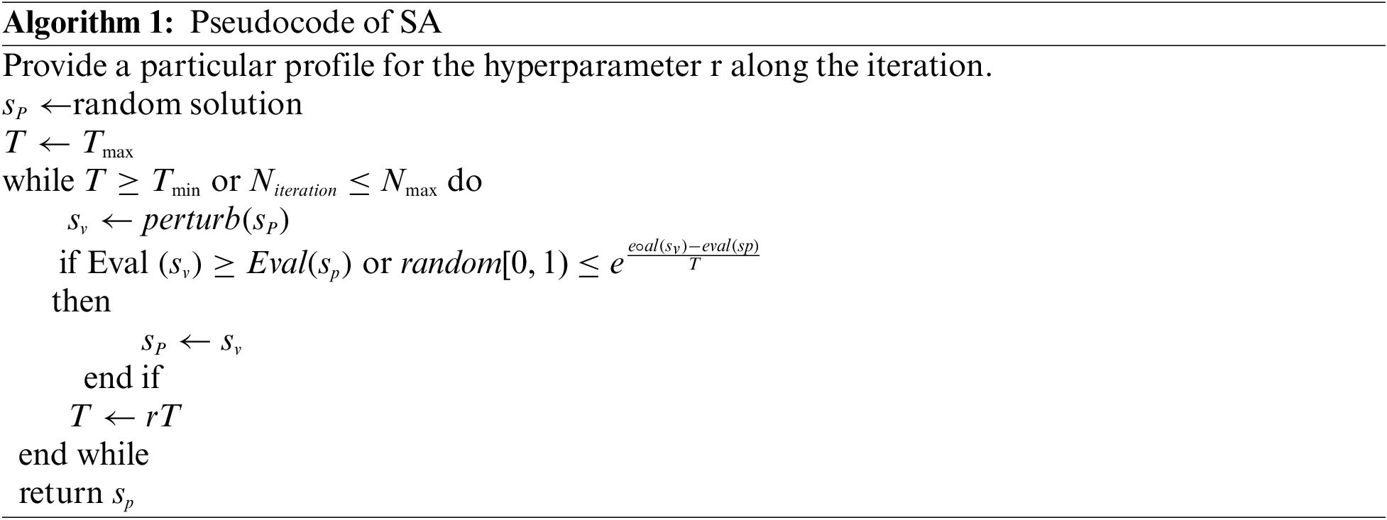
The SA is utilised in this work to optimally adjust the ELM parameters such as several neurons, alpha, pairwise metric, and batch size. A search algorithm describes a process for defining a solution for the problem while discovering a mathematically well-defined searching space. Hill Climbing (HC) or Steepest ascent is an example of this model. It initiates with a primary solution replaced iteratively through the best neighbour until no more improvement is possible. This algorithm is completed if there exists an assurance of the result, a possible solution, and an optimum when it is assurance for defining an optimum amongst each solution. HC is either optimal or complete. Another searching technique is the Random Walk; at each step, a novel solution has been completely sampled at arbitrary or as a blind perturbation of the existing solution. This process is optimal and whole and provides an immense quantity of computation resources.

The SA is the middle ground between the two techniques; the metallurgy's annealing process stimulates this technique. The gradual cooling assists the condition for reaching a lower energy state, so metallic alloy atomic composition generates solid alloys with various properties of interest to industry. Once the heating and cooling process takes place rapidly, the metal alloy, in the end, may become brittle and won’t have a better internal structure. On the other hand, a low temperature makes them hard to accept candidate solutions of the worst quality. Hence, if the temperature is high, the model performs a random search at an early stage. In the end, if the temperature is low, it becomes similar to HC.

Algorithm 1 defines the pseudocode for SA. The process begins by producing an arbitrary primary solution and assigning the maximum value (Tmax) for the current temperature. It iteratively attempts to increase the existing solution still the temperature reaches a value of Tminor until a specific amount of iterations is accomplished [23]. It employs a perturbation process to the present solution producing an adjacent solution. Once the novel solution is superior to the present one, it exchanges the present solution. Or else, assume a maximized problem, it exchanges the existing solution with probability

p=eeval(SV)−eval(sp)T,(15)

Let T be the current temperature, sP shows the existing solution, and sv indicates the candidate solution. The eval function measures the comparative quality of the presented. Lastly, the present temperature T is different by a factor r.

With a suitable temperature variation policy, the model can escape from local minima and progress to the best candidate solution, finally finding a better quality solution. To use the idea of annealing schedule and Genetic Programming (GP) to select amongst exchanging an individual parent with its children or not. In other words, the author uses SA to evolve the expression tree’s mathematical constant. The SA method would derive a fitness function (FF) for obtaining superior classifier results. It sets positive values for denoting superior outcomes of candidate solutions. During this article, the reduction of the classifier error rate has been regarded as the FF as provided below in Eq. (16). A good solution contains less error rate, and the worst one gains a higher error rate.

fitness(xi)=numberofmisclassifiedsamplesTotalnumberofsamples∗100(16)

4  Experimental Validation

The presented model is simulated using the Python tool. Before the experimental validation process, data augmentation was carried out to increase the size of the dataset. The proposed approach uses a benchmark tongue image dataset containing images under various 12 class labels. We have taken 78 images in this study under CHD, pneumonia, and health class.

Fig. 3 depicts some original sample images. During this work, the data augmentation takes place in different ways:

•   zoom_range = 0.15,

•   rotation_range = 90,

•   horizontal_flip = True,

•   height_shift_range = 0.2,

•   fill_mode = “nearest”,

•   shear_range = 0.15,

•   width_shift_range = 0.2

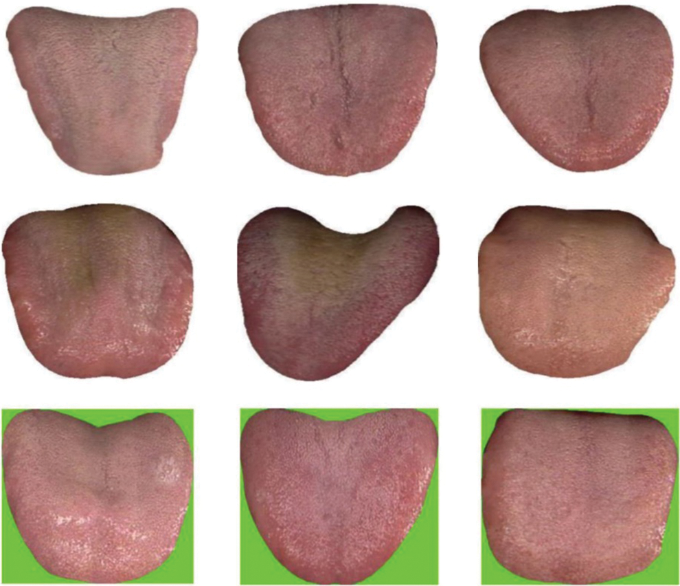
Figure 3: Original images

Figs. 4 and 5 demonstrate some sample pre-processing and extracted feature images.

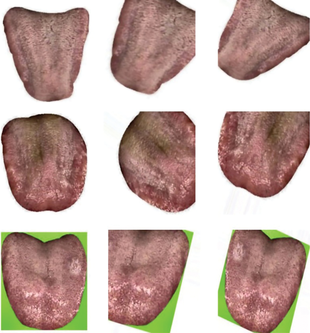
Figure 4: Pre-processed images

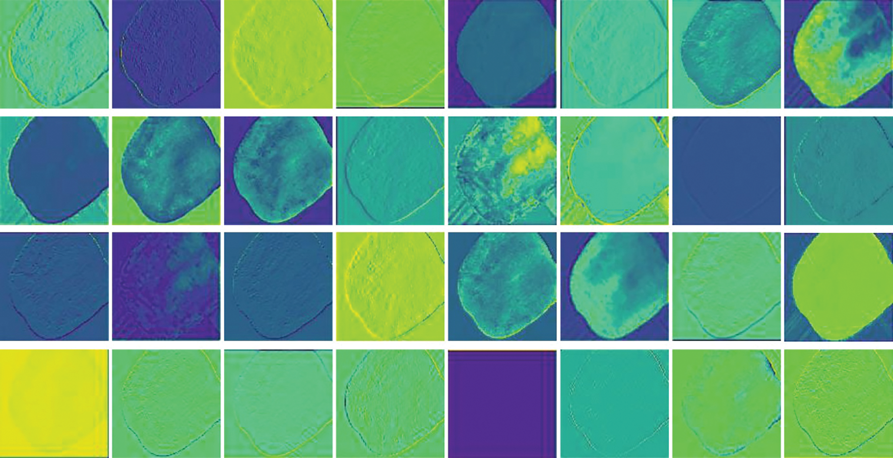
Figure 5: Extracted features

Table 1 provides the optimal parameter values of the ELM approach derived by the SA. The experimental values indicated different values obtained by the SA at the execution time. The optimal values are marked in bold font. The optimal ELM parameters are n_neurons: 0.0764, pairwise_metric: city block; batch size: 64, and score: 0.9859. Table 2 depicts a detailed description of the dataset.

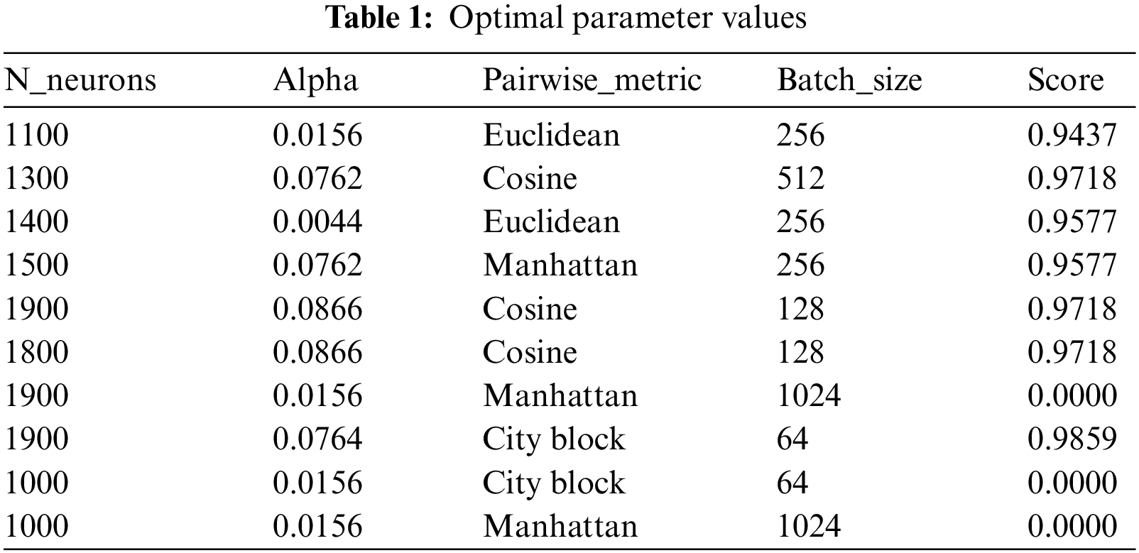
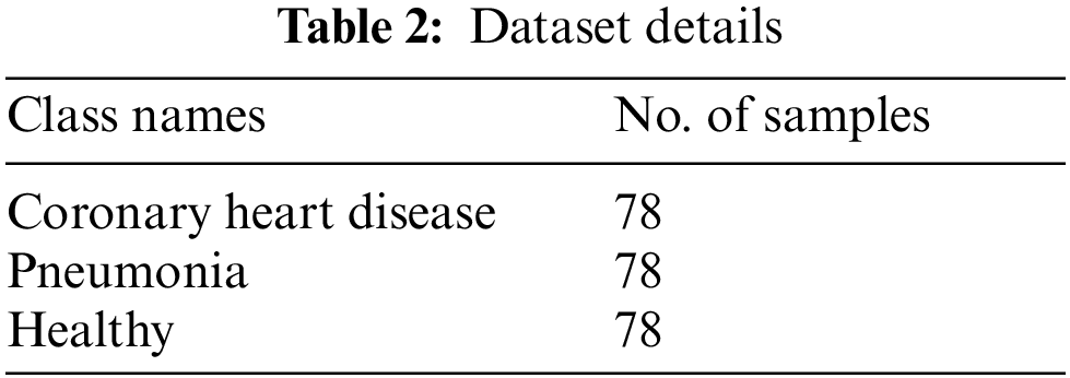
Fig. 6 represents a detailed investigation of the SADTL-TIADD approach during the Training phase. Fig. 6a portrays the confusion matrix offered by the SADTL-TIADD technique. The figure demonstrated that the SADTL-TIADD model had identified 54 instances under class 1, 57 instances under class 2, and 52 instances under class 3. Afterwards, Fig. 6b illustrates the precision-recall analysis of the SADTL-TIADD model. The figures stated that the SADTL-TIADD technique had obtained maximal performance over distinct classes. Lastly, Fig. 6c illustrates the ROC investigation of the SADTL-TIADD model. The figure revealed that the SADTL-TIADD technique had obtained superior ROC values under distinct class labels.

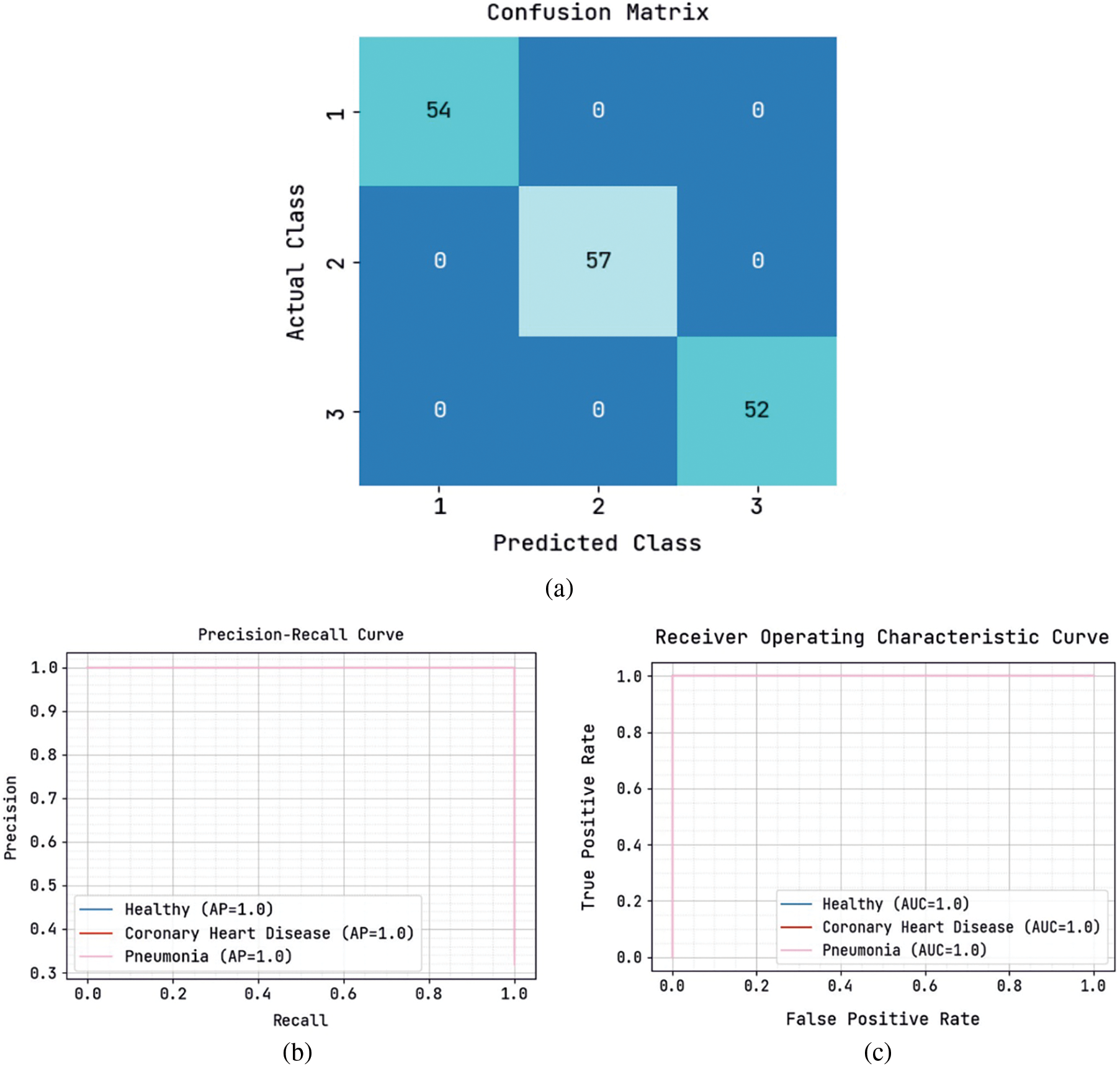
Figure 6: Classification analysis of SADTL-TIADD approach under training phase (a) confusion matrix, (b) precision-recall, and (c) ROC curve

Fig. 7 showcases a brief investigation of the SADTL-TIADD technique during the testing phase. Fig. 7a depicts the confusion matrix offered by the SADTL-TIADD system. The figure stated that the SADTL-TIADD methodology had identified 24 instances under class 1, 21 instances under class 2, and 25 instances under class 3. Next, Fig. 7b demonstrates the precision-recall analysis of the SADTL-TIADD approach. The figures reported that the SADTL-TIADD model had obtained higher performance over distinct classes. Finally, Fig. 7c depicts the ROC investigation of the SADTL-TIADD technique. The figure stated that the SADTL-TIADD model had obtained higher ROC values under distinct class labels.

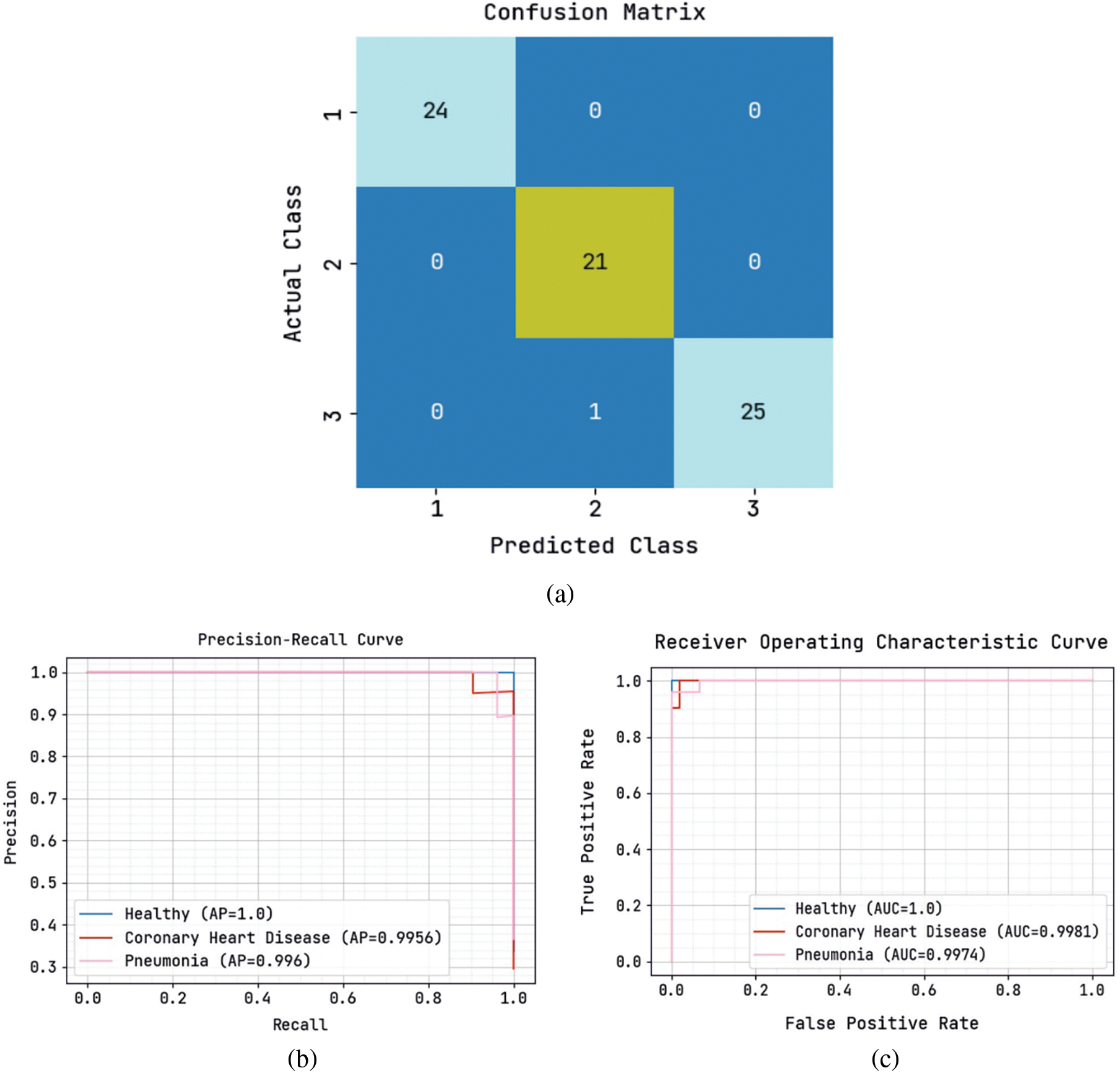
Figure 7: Classification analysis of SADTL-TIADD approach under testing phase (a) confusion matrix, (b) precision-recall, and (c) ROC curve

Table 3 provides comprehensive classification results offered by the SADTL-TIADD model. The experimental values indicate that the SADTL-TIADD approach has achieved effectual performance in all aspects.

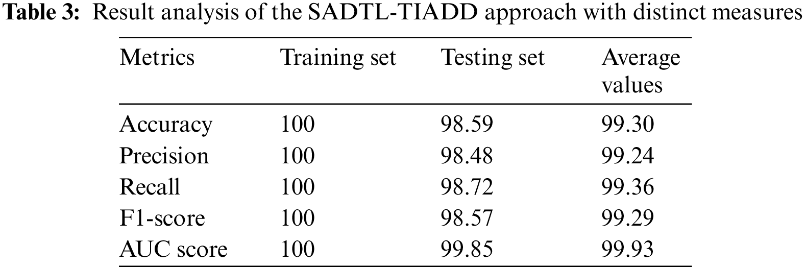
For sample, on the training set, the SADTL-TIADD model has achieved accuy of 100%, precn of 100%, recal of 100%, F1score of 100%, and AUCscore of 100%. At the same time, on the testing set, the SADTL-TIADD approach has accomplished accuy of 98.59%, precn of 98.48%, recal of 98.72%, F1score of 98.57%, and AUCscore of 99.85%.

To demonstrate the enhanced performance of the SADTL-TIADD approach, a brief comparison study with recent models is carried out in Table 4 [18]. The experimental values inferred that the GF, SVM, Geometric Features using Sparse Representation-based Classification (GF-SRC), and K-Nearest Neighbor (KNN) models had reported lower accuy values of 75.96%, 76.16%, 79.34%, and 74.69% respectively. Moreover, the GA-SVM model has reached a moderately improved accuy of 82.93%. Next, the Automated IoT and Synergic Deep Learning based Tongue Color Image (ASDLTCI) model has resulted in a reasonable accuy of 97.93%.

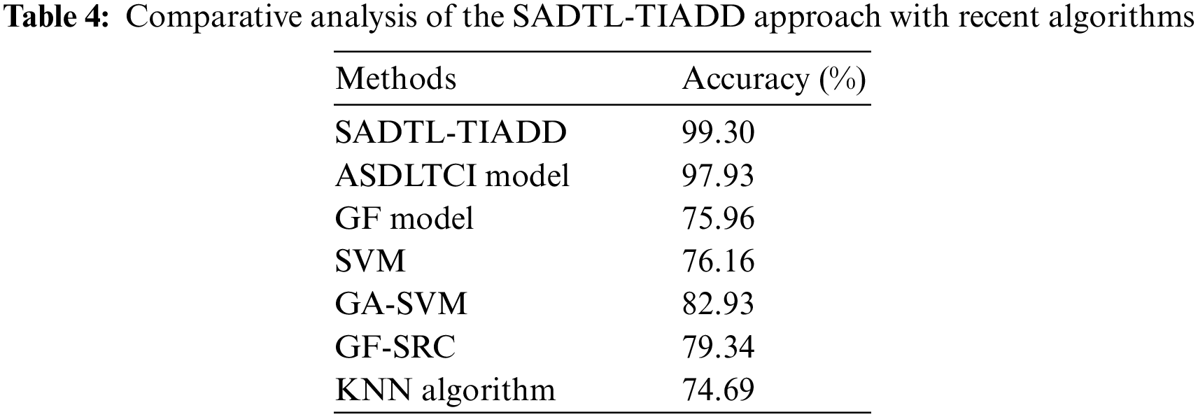
However, the presented SADTL-TIADD model outperformed the other models with a higher accuy of 99.30%. From the detailed results and discussion, it can be confirmed that the SADTL-TIADD model has shown enhanced performance over other models.

5  Conclusion

This study established a novel SADTL-TIADD system for detecting and classifying diseases using tongue images. To accomplish this, the SADTL-TIADD approach initially BF-based pre-processing and CLAHE-based contrast enhancement. Next, the presented SADTL-TIADD technique employed an EfficientNet-based feature extractor to generate useful feature vectors. For disease detection and classification, the SA with the ELM model is applied, and using SA enhances the classification efficiency. A wide-ranging set of simulations was performed to ensure the improved performance of the SADTL-TIADD system. The experimental outcomes highlighted the superior of the presented SADTL-TIADD algorithm over the compared methods. Therefore, the SADTL-TIADD technique can be employed for productive tongue image analysis. In the future, the SADTL-TIADD methodology's performance will be enhanced using feature reduction techniques.

Funding Statement: The authors received no specific funding for this study.

Conflicts of Interest: The authors declare they have no conflicts of interest to report regarding the present study.

References

1. T. Jiang, X. J. Guo, L. P. Tu, Z. Lu, J. Cui et al., “Application of computer tongue image analysis technology in the diagnosis of NAFLD,” Computers in Biology and Medicine, vol. 135, no. 1, pp. 1–12, 2021. [Google Scholar]

2. E. Vocaturo, E. Zumpano and P. Veltri, “On discovering relevant features for tongue colored image analysis,” in Proc. of the 23rd Int. Database Applications & Engineering Symp., Athens Greece, pp. 1–8, 2019. [Google Scholar]

3. J. Hu, Z. Yan and J. Jiang, “Classification of fissured tongue images using deep neural networks,” Technology and Health Care, vol. 30, no. 8, pp. 271–283, 2022. [Google Scholar] [PubMed]

4. S. Dalam, V. Ramesh and G. Malathi, “Tongue image analysis for COVID-19 diagnosis and disease detection,” International Journal of Advanced Trends in Computer Science and Engineering, vol. 9, no. 5, pp. 7924–7928, 2020. [Google Scholar]

5. Q. Xu, Y. Zeng, W. Tang, W. Peng, T. Xia et al., “Multi-task joint learning model for segmenting and classifying tongue images using a deep neural network,” IEEE Journal of Biomedical and Health Informatics, vol. 24, no. 9, pp. 2481–2489, 2020. [Google Scholar] [PubMed]

6. H. Li, G. Wen and H. Zeng, “Natural tongue physique identification using hybrid deep learning methods,” Multimedia Tools and Applications, vol. 78, no. 6, pp. 6847–6868, 2019. [Google Scholar]

7. J. Li, Q. Chen, X. Hu, P. Yuan, L. Cui et al., “Establishment of non-invasive diabetes risk prediction model based on tongue features and machine learning techniques,” International Journal of Medical Informatics, vol. 149, no. 1, pp. 1–7, 2021. [Google Scholar]

8. D. C. Braz, M. P. Neto, F. M. Shimizu, A. C. Sá, R. S. Lima et al., “Using machine learning and an electronic tongue for discriminating saliva samples from oral cavity cancer patients and healthy individuals,” Talanta, vol. 243, pp. 123327, 2022. [Google Scholar] [PubMed]

9. J. Heo, J. H. Lim, H. R. Lee, J. Y. Jang, Y. S. Shin et al., “Deep learning model for tongue cancer diagnosis using endoscopic images,” Scientific Reports, vol. 12, no. 1, pp. 1–10, 2022. [Google Scholar]

10. S. Balu and V. Jeyakumar, “A study on feature extraction and classification for tongue disease diagnosis,” in Intelligence in Big Data Technologies—Beyond the Hype. Singapore: Springer, pp. 341–351, 2021. [Google Scholar]

11. C. Song, B. Wang and J. Xu, “Classifying tongue images using deep transfer learning,” in 2020 5th Int. Conf. on Computational Intelligence and Applications (ICCIA), Beijing, China, pp. 103–107, 2020. [Google Scholar]

12. X. Huang, L. Zhuo, H. Zhang, X. Li and J. Zhang, “Lw-TISNet: Lightweight convolutional neural network incorporating attention mechanism and multiple supervision strategy for tongue image segmentation,” Sensing and Imaging, vol. 23, no. 1, pp. 1–20, 2022. [Google Scholar]

13. S. Balasubramaniyan, V. Jeyakumar and D. S. Nachimuthu, “Panoramic tongue imaging and deep convolutional machine learning model for diabetes diagnosis in humans,” Scientific Reports, vol. 12, no. 1, pp. 1–18, 2022. [Google Scholar]

14. C. Zhou, H. Fan and Z. Li, “Tonguenet: Accurate localization and segmentation for tongue images using deep neural networks,” IEEE Access, vol. 7, pp. 148779–148789, 2019. [Google Scholar]

15. S. N. Deepa and A. Banerjee, “Intelligent decision support model using tongue image features for healthcare monitoring of diabetes diagnosis and classification,” Network Modeling Analysis in Health Informatics and Bioinformatics, vol. 10, no. 1, pp. 1–16, 2021. [Google Scholar]

16. W. Tang, Y. Gao, L. Liu, T. Xia, L. He et al., “An automatic recognition of tooth-marked tongue based on tongue region detection and tongue landmark detection via deep learning,” IEEE Access, vol. 8, pp. 153470–153478, 2020. [Google Scholar]

17. X. Wang, J. Liu, C. Wu, J. Liu, Q. Li et al., “Artificial intelligence in tongue diagnosis: Using deep convolutional neural network for recognizing unhealthy tongue with tooth-mark,” Computational and Structural Biotechnology Journal, vol. 18, pp. 973–980, 2020. [Google Scholar] [PubMed]

18. R. F. Mansour, M. M. Althobaiti and A. A. Ashour, “Internet of things and synergic deep learning based biomedical tongue color image analysis for disease diagnosis and classification,” IEEE Access, vol. 9, pp. 94769–94779, 2021. [Google Scholar]

19. K. Shirai, K. Sugimoto and S. I. Kamata, “Adjoint bilateral filter and its application to optimization-based image processing,” APSIPA Transactions on Signal and Information Processing, vol. 11, no. 1, pp. 1–27, 2022. [Google Scholar]

20. U. Kuran and E. C. Kuran, “Parameter selection for CLAHE using multi-objective cuckoo search algorithm for image contrast enhancement,” Intelligent Systems with Applications, vol. 12, no. 13, pp. 200051, 2021. [Google Scholar]

21. M. Tan and Q. Le, “Efficientnet: Rethinking model scaling for convolutional neural networks,” in Int. Conf. on Machine Learning, California, United States, pp. 6105–6114, 2019. [Google Scholar]

22. N. Kardani, A. Bardhan, B. Roy, P. Samui, M. Nazem et al., “A novel improved Harris Hawks optimization algorithm coupled with ELM for predicting permeability of tight carbonates,” Engineering with Computers, vol. 38, pp. 1–24, 2021. [Google Scholar]

23. H. Lv, X. Chen and X. Zeng, “Optimization of micromixer with Cantor fractal baffle based on simulated annealing algorithm,” Chaos, Solitons & Fractals, vol. 148, no. 1, pp. 111048, 2021. [Google Scholar]