Long-Term Energy Forecasting System Based on LSTM and Deep Extreme Machine Learning

1  Introduction

Building sector is considered as one of the huge energy consuming entities nowadays, accounting for about 40% of international energy consumption [1]. Indeed, energy consumption studies problems have become a central aim of studies in recent decades. As energy is one of the highly important resources for industrial production, anticipating energy consumption is an important task for macro planning of industrial and energy sectors [2]. Energy efficiency has become a challenge of high priority and importance achieving a cleaner and more sustainable way of life. As it is a massively important resource, its demand is increasing daily. Therefore, saving energy is not just important to promote a green atmosphere for future sustainability but also necessary for household consumers and power generation companies. Predicting the energy consumption for buildings is a great way for building managers to choose all types of equipment wisely. Moreover, this is an efficient and crucial way to avoid wasting building energy and improve energy efficiency. As a sub-area of energy consumption, building energy consumption accounts for a significant proportion [2]. Researchers have developed several powerful simulation tools, such as Energy Plus [3], DEST [4], and eQuest [5], relying on the fundamental concepts of the thermodynamic equilibrium equation and the heat equation. Hence, these tools can accurately compute the building energy consumption with exact boundary conditions and offer important insights into energy consumption models with physical meanings. Still, there are drawbacks related to these various tools. They react exceptionally to boundary conditions that are based on expertise. Furthermore, the simulations take a lot of time, which refutes the main idea of rapid and precise computing in terms of big data. As data mining transforms several disciplines, data-driven approaches for predicting building energy consumption have become mainstream [6]. Generally, smart homes have different and huge energy necessitates managing all modules and present new advances in an organized manner by making optimal application of all these energy sources. Thus, an efficient predictive concept for energy management in a smart home is needed. Moreover, due to the increase in data and processing power of computers, machine learning and deep learning have been applied in different fields [7] such as construction [8], security [9–11], medical [12], economics [13] and image recognition [14]. The recent efficiencies of deep learning in multiple fields have attracted scientists to monitor energy consumption, and its promising potential is demonstrated by the plethora of proposed models and the increasing diversity of research. In this context, deep learning plays an important role in the domain of energy consumption. It offers many accurate models to achieve this goal. Deep learning methods can predict both linear and nonlinear correlations, making it a useful choice for energy prediction. Deep neural networks (DNN) improve forecasting accuracy and reduce operating costs by reducing the number of errors. In forecasting research, DNN have been considered widely for their performance in solving nonlinear relationship problems.

Hence, this article aims to propose a hybrid model for reducing energy consumption and ensuring its efficient use. The major contributions of the proposed model are underlined as follows:

1)   An acquisition and refinement layer is employed, which refines the data by substituting past values, normalizing, and organizing the data into a continuous windowing sequence.

2)   A LSTM network is designed for energy forecasting that extracts the most discriminating spatial-temporal features from the power load sequence and makes a block of feature map.

3)   DELM network has been applied for sequence learning, which obtains the spatiotemporal features (feature map) from the LSTM network. The DELM network is adequate for learning the sequence patterns and provides an effective energy prediction.

We prove through experiments that the proposed model shows excellent results and outperforms the state of the art by recording the lowest value of MSE and RMSE on the most demanding data set. It reveals the suitability of the method to effectively manage the energy infrastructure and ensure the saving of large amounts of energy waste. By applying our proposed method, we achieved accurate and quick calculation results. The objective is to provide maximum user comfort at the cost of minimum energy consumption. With regard to the rest of the paper, Section 2 discusses related works, which treat models used for energy prediction. Section 3 provides an overview of the proposed system of energy forecasting. Section 4 presents the performance evaluation of the model proposed and discusses the main results. Finally, Section 5 concludes the paper.

2  Related Work

A detailed overview of the most important methods for optimizing and predicting energy consumption was carried out in [15]. In [16], a comparison between PSOANN and a simple ANN with GA-ANN succeeded (GA was implemented for the same goal as PSO). Two databases have been applied to predict hourly electricity consumption. An optimization strategy was developed in [17]. It was called teach-learn based optimization. It employs evolutionary algorithms with BPNN to improve convergence speed and prediction performance. A basic aggregated model was designed along with five improved versions. A short-term energy consumption prediction model was endowed by [18]. It used a multilayer perceptron (MLP), a scaled conjugate gradient and Levenberg-Marquardt backpropagation algorithms. An energy forecasting technique for smart homes proposed in [19]. They introduced artificial neural networks to forecast the energy consumption in different time intervals daily or weekly. The dynamic neural network and the Energy Plus program were useful in predicting the building energy load and the Taguchi method to measure the effect of parameters on the load [20]. In [21], the authors presented a comparison of ANN, SVM and ARIMA models to forecast heating and cooling energy consumption in Chinese office buildings in Shanghai, Nanjing and Changsha. All models were evolved with IBM SPSS Modeller. The results showed that the ANN is better than the SVM and that both outperformed the ARIMA with a MAPE of 0.15%–0.11percentage, 0.21%–0.18% and 0.41%–0.33%, respectively (test samples in the first and second month). Another effective hybrid approach in [22] used an autoregressive integrated moving average (ARIMA) to forecast energy consumption. An IoT-based home energy management method for energy consumption optimization of electronic devices in smart homes in [23] used a hybrid artificial neural network and particle swarm optimization algorithms. The model presented the early design of energy efficient buildings. Besides simple neural networks, other algorithms for energy consumption prediction have also been successful, such as the extreme learning machine-based model in [24], the Bat algorithm, and fuzzy logic control to improve energy consumption utilizing temperature, lighting, and air quality in [25]. Through efficient prediction, various approaches provide rough directions and features for energy consumption prediction, such as weather information and power data. Due to their disorganized data usage, these methods are also less effective in predicting. The literature discussed above indicates that most prediction methods rely on statistical features and utilize machine learning techniques to predict energy consumption. Due to its high accuracy and performance in energy and electric systems, we introduce a hybrid deep learning model based on LSTM and DELM to overcome several challenges. As a result of weather conditions and occupant behavior, the collected energy consumption data can contain abnormalities and redundancies, leading to incorrect energy predictions. So, consumer and supplier power management fails. Resolving this issue requires removing noise and handling missing values. When it comes to smart grid planning and electricity marketing, statistical machine learning techniques like linear regression and clustering have limited effectiveness. Several LSTM layers are added for feature extraction. In this paper, we propose a method that predicts power consumption using the LSTM-DELM sequential learning algorithm. By combining forward and backward interpretations at the end, the LSTM-DELM learns the input sequence, and then predicts output power by concatenating them. Experiments have also shown that the proposed method is superior to existing approaches. By using our method, MSE and RMSE are the lowest values obtained, proving that it predicts accurately energy consumption.

3  Proposed System

In this section, the novel hybrid model applied to predict energy is detailed. First, we present the models employed in the feature extraction and learning task. Then, a great concise description of our own system is developed. . In this study, we have followed these steps in order to obtain results of prediction of energy as presented in Fig. 1.

Figure 1: Methodology of prediction

The proposed energy prediction system is described in Fig. 2. It involves of three steps:

1.    Step1: For data management and energy usage response, the first step is to collect data from sensors and smart meters. Further refinement is performed so that user behavior can be stabilized and removed.

2.    Step 2: LSTM is used to extract features from the energy data.

3.    Step 3: This step involves predicting future energy consumption using the input data.

Figure 2: The proposed energy prediction system

3.1 Data Collection and Refinement

This part provides an explanation of data collection from sources such as gauges and installed sensors. Data pre-processing is also explained. To collect data, wires are run across the building floors in a single edge with the motherboard, and the meter with few sensors is installed to read and measure energy usage above the building structure, where the data is usually collected at minute resolutions. Normally, climate conditions affect the data collected by sensors and meters, occupant behavior, redundancy, broken wire or short circuit, leading to noise in the variable values. Solving this problem is crucial for accurate forecasts; Therefore, we refine the data before the actual processing.

3.2 Feature Extraction and Learning

3.2.1 Sequence Modeling Through LSTM

As a dimensionality reduction technique, feature selection can be useful for reducing the dimensions of time series meteorological datasets [26]. By providing only relevant features as input to the prediction model, the feature selection improves the capability and reduces the complexity [27]. To model the sequential data, a form of recurrent neural networks (RNNs) such as LSTM was chosen as it is the most stable and powerful network that understands and processes the long-range information. LSTM has the ability to learn long-term sequence information.

This section defines the internal design of LSTM in sequence analysis. LSTM is a complex version of RNN, with more layers inside. It proposes special units called memory blocks in the recurring layer to surmount vanishing/exploding gradient problems. Fig. 3 presents the structure of a memory block. Memory cells are integrated in the self-connected memory blocks. Three special multiplicative units, called gates, are introduced to store temporal sequences. The three gates have these functions as follows:

Input gate: This gate controls the information flow into the memory cell.

Output gate: This gate controls the information flow into the remainder of the networks.

Forget gate: This gate selects the cell state at the prior moment and retains a portion of the information into the current moment.

Figure 3: Structure of a memory block

These gates are equal to multiplying the previous information by a number ranging from 0 to 1. If the number is zero, all previous information flow is discarded. If the number is 1, the entire flow of information is kept. The three gates all use sigmoid functions that make the data limited to the range of 0–1. The sigmoid function is presented as:

ω(x)=11+e−x(1)

at, bt,ct  are respectively the input gate, forget gate, and output gate, ϕt is the intermediate value during when calculating,

at=φ(SaTt+Vagt−1+bit)(2)

ϕt=tanh(SzTt+Vzgt−1+biz)(3)

bt=φ(SbTt+Vbgt−1+bib)(4)

ϕt=at∗ϕt+bt∗ϕt−1(5)

ct=φ(ScTt+Vcgt−1+bic)(6)

gt=ct∗tanh(ϕt)(7)

where Si, Vi,  Sz, Vz, Bb, Vb, Sc and Vc are weight matrices, bit, bz, bib and bic are bias vectors. Tt  is the current input. gt  and gt−1 are the outputs at the current time t and the previous time t − 1, respectively. The hyperbolic tangent function is presented as follows:

tanh⁡(x)=ex−e−xex+e−x(8)

3.2.2 Deep Extreme Machine Learning Network

Deep extreme learning networks receive the features obtained from these LSTM layers. It is a variation of the Extreme Learning Machine (ELM). It has been adopted in many domains. The traditional algorithm based on artificial neural networks necessitates more training samples; slower learning times, and can lead to overfitting of a learning model [28]. Deep ELM, as presented in Fig. 4 is one of the latest and highly important iterations in the ELM evolution. DELMs are based on the concept of MLELMs with the application of KELM as the output layer [29]. The number of hidden layers relies on the problem under study. Here we adopted seven hidden layers in the proposed model. We used trial and error to choose the number of nodes in the hidden layers. We adopted the process described by [30], for the calculation method of hidden layers of the Deep Extreme Learning Machine (DELM) network.

Figure 4: The DELM model

The concept of ELM was first specified in [31]. The ELM is widely adopted in many fields for classification and regression purposes because an ELM learns very rapidly and it is computationally efficient. The ELM model is presented in Fig. 5. It includes an input layer, a single hidden layer, and an output layer.

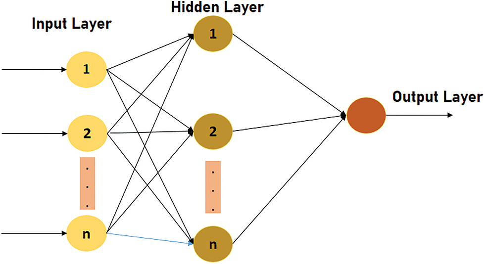
Figure 5: The ELM structure

Where p represents input layer nodes, q represents hidden layer nodes, and r indicates output layer nodes. First of all, consider {E, F} = {Ei,Fi}  where (i = 1, 2, 3 … p), E = [ei1,ei2,ei3 ,…,eip}] is the output feature and the matrix F = [fi1,fi2,fi3,…,fip}]. The matrix E and F are presented as Eqs. (9) and (10):

E=[e11e12..e1pe21e22..e2pe31e32..e3pe41e42..e4p........eq1eq2..eqp](9)

F=[f11f12..f1pf21f22..f2pf31f32..f3pf41f42..f4p........fk1fk2..fkp](10)

where q and k indicate the output and input matrix dimensions, respectively. The ELMs randomly assign weights between input layers and the hidden layer. The weights t are represented among the ith neurons of the input layer and jth neurons output hidden layer. ELM considers weights between the output layer and the hidden layer of neurons, which is expressed in Eq. (11):

T=[T11T12..T1qT21T22..T2qT31T32..T3qT41T42..T4q........Tl1Tl2..Tlq](11)

Ω=[Ω11Ω12..Ω1kΩ21Ω22..T2kΩ31Ω32..Ω3kΩ41Ω42..Ω4k........Ωq1Ωq2..Ωqk](12)

The ELM randomly sets the bias of the hidden layer as Eq. (13):

F=[f1,f2,f3,…,fq]T(13)

S=[s1,s2,s3,…,sQ]k∗p(14)

Each column of the matrix S is presented as follows:

s=[s1js2js3j...skj]=[∑iqΩr1g(tra1+fr)∑iqΩr2g(tra1+fr)∑iqΩr3g(tra1+fr)...∑iqΩrkg(tra1+fr)]i=1,2,3,…,Q(15)

Transpose of the matrix T is denoted by μ:

μ=[s1,s2,s3,…,sQ]T(16)

Taking Eqs. (6) and (7) into account, we obtain (9):

DΩ=μ(17)

Ω=D+μ(18)

The regularization term Ω is used to make the network more generalized and stable. With the combination of the benefits of ELMs and deep learning (DL), we obtain the second layer as expressed in Eq. (11):

D1=SΩ(19)

where Ω+ the generalized inverse of matrix Ω. The output of hidden layer 2 is obtained using Eq. (18) and the activation function inverse.

h(T1S+F1)=D1(20)

In Eq. (20), the variables T1 S, F1 and D1 are weight matrices of the initial 2 hidden layers, the bias of the neurons of the first hidden layer, the output of the initial hidden layer, and the projected output of the 2nd hidden layer.

TDE=h−1(D1)DE+(21)

DE+ is the inverse of DE, and the activation function h(x) is used in Eq. (22). Therefore, given any suitable activation function h(x), the output of the second hidden layer will be as follows:

D2=H(TDEDE)(22)

The update of the weight matrix Ω among the second and third hidden layers is performed in Eq. (23), where D2+ represents the inverse of  D2. so, the predicted value of the third layer is defined as:

Ωnew=D2+S(23)

D3=SΩnew+(24)

where Ωnew+ new represents the inverse of the weight matrix Ωnew. Then, the DELM represents the matrix TDE = [F2, T2]. The output of the third layer is obtained using Eqs. (9)–(10).

D3=h−1(D2T2+F2)=h(TDE1DE1)(25)

TDE1=Ω−1(D3)DE1+(26)

where D2 is the anticipated output of hidden layer 2, T2 represents the weight between the second and third hidden layers, and F2  is the bias of the neurons of the third hidden. DE1+ is the inverse of DE1 , and h−1 represents the inverse of the activation function h(x). The logistic sigmoid function in Eq. (27) is used, and the third hidden layer output is obtained as follows:

g(x)=11+e−x(27)

D3=h(TDEDE1)(28)

The resultant weight matrix between the third hidden layer and the output layer is represented in Eq. (29). The projected output of the third hidden layer is expressed as follows:

Ωnew=D4T(1β+D4TD4)−1S(29)

D4=SΩnew+(30)

Ωnew+ is the inverse of the weight matrix Ωnew. Here, the DELM represents the matrix TDE = [F2, T2].The output of the fourth layer is calculated using Eqs. (31)–(32).

D4=h−1(D3T3+F3)=h(TDE2DE2)(31)

TDE2=Ω−1(D4)DE2+(32)

In Eq. (28), D3 is the predicted output of the third hidden layer, the weights between the third and fourth hidden layers are represented as T3 and F3 is the bias of the neurons of the third hidden layer. DE1+ is the inverse of DE1 and h−1 is the inverse of the activation function h(x). The logistic sigmoid function is used. The output of the third and fourth layers is calculated as Eq. (33):

D4=h(TDE2DE2)(33)

Now, the output weight matrix among the fourth and the fifth layer is determined using Eq. (34). The projected output of the fifth layer is presented in Eq. (35). The predicted output of the DELM network is defined in Eq. (36).

Ωnew=D5T(1β+D5TD5)−1S(34)

D5=SΩnew+(35)

Ωnew+ is the inverse of the weight matrix Ωnew. Here, the matrix TDE3 = [F3, T3] is presented. The output of the fifth layer is calculated using Eqs. (36)–(37)

D5=h−1(D4T4+F4)=h(TDE3DE3)(36)

TDE3=Ω−1(D3)DE3+(37)

The output of the fourth and fifth layers is calculated as Eq. (38)

D5=h(TDE3DE3)(38)

Here, the output weight matrix among the fifth and the sixth layer is determined using Eq. (39). The projected output of the sixth layer is presented in Eq. (40). The predicted output of the DELM network is defined in Eq. (41).

Ωnew=D6T(1β+D5TD5)−1S(39)

D6=SΩnew+(40)

g(x)=D5Ωnew(41)

In this section, we have discussed the calculation process for the seventh hidden layer of the DELM network. To demonstrate the calculation process of DELM, cycle theory was applied. In order to obtain the hidden layer’s parameters and ultimately the final result of the DELM network, Eqs. (26)–(38) are utilized. This process is illustrated in Fig. 6.

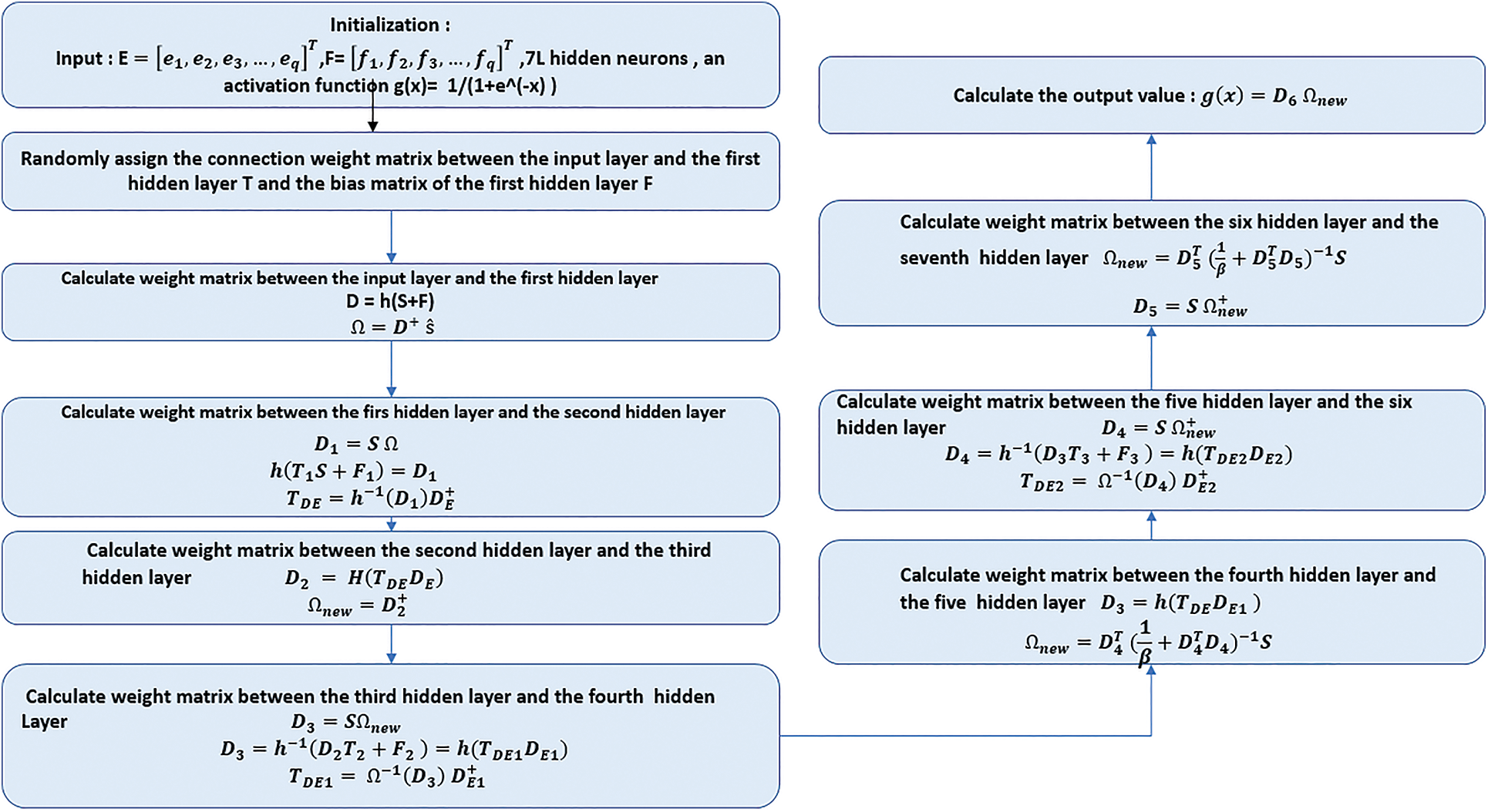
Figure 6: DELM proposed algorithm

4  Discussion

This section describes the detailed experimental evaluation of the proposed model on this dataset [32]. We evaluate and analyze the proposed LSTM-DELM network using different types of experiments to measure its performance using the household performance dataset. It has been collected from 2006 to 2010. It contains 2075259 instances, with 25979 instances containing missing values, accounting for 1.25% of the whole data. In Table 1, the variables used in this dataset are listed with their detailed comments. In addition, the quantitative details of the household electricity dataset are provided. The data set is divided into two parts:

•   Training set: 70% of the data is selected as the training set.

•   Test set: 30% of the data set is selected and used as the test set for evaluation of the detector’s performance. Training was performed over 100 epochs, with each epoch running through all training images containing 350 steps in each epoch.

We analyze the results of our proposed method. The proposed method is implemented in Python (version 3.5) using Keras (Deep Learning Framework) powered by TensorFlow. In order to evaluate the forecasting models’ performance, these assessment criteria are used: The MAE is based on the absolute error and can show the normal separation between the expected value and the actual value. To analyze the precision of different anticipating standards, RMSE is commonly used as an expectation quality estimation. Because the measurement mathematically enhances errors, huge errors are punished. R² measures how closely a model approximates the real information, giving a metric of its consistency.

MAE=1n∑1n⁡(Si−Ti)(42)

MSE=1n∑1n⁡(Si−Ti)2(43)

RMSE=(1n∑1n⁡(Si−Ti)2)(44)

where n represents the number of observations, T denotes the actual value, and S denotes the estimated value. Accuracy metrics values are given in Table 2.

As training time, LSTM-DELM achieves 3.1 with 1.5129 as RMSE. Compared to other models, as illustrated in Fig. 7, it outperforms other ones.

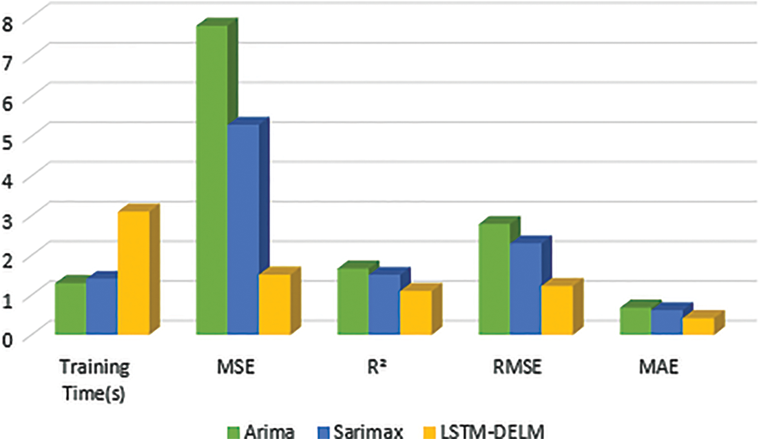
Figure 7: Results of energy prediction

A learning curve is most commonly illustrated by loss over time. Our model error is measured by loss. Therefore, our model’s performance will improve as our loss decreases. Fig. 8 illustrates how the learning process is expected to behave.

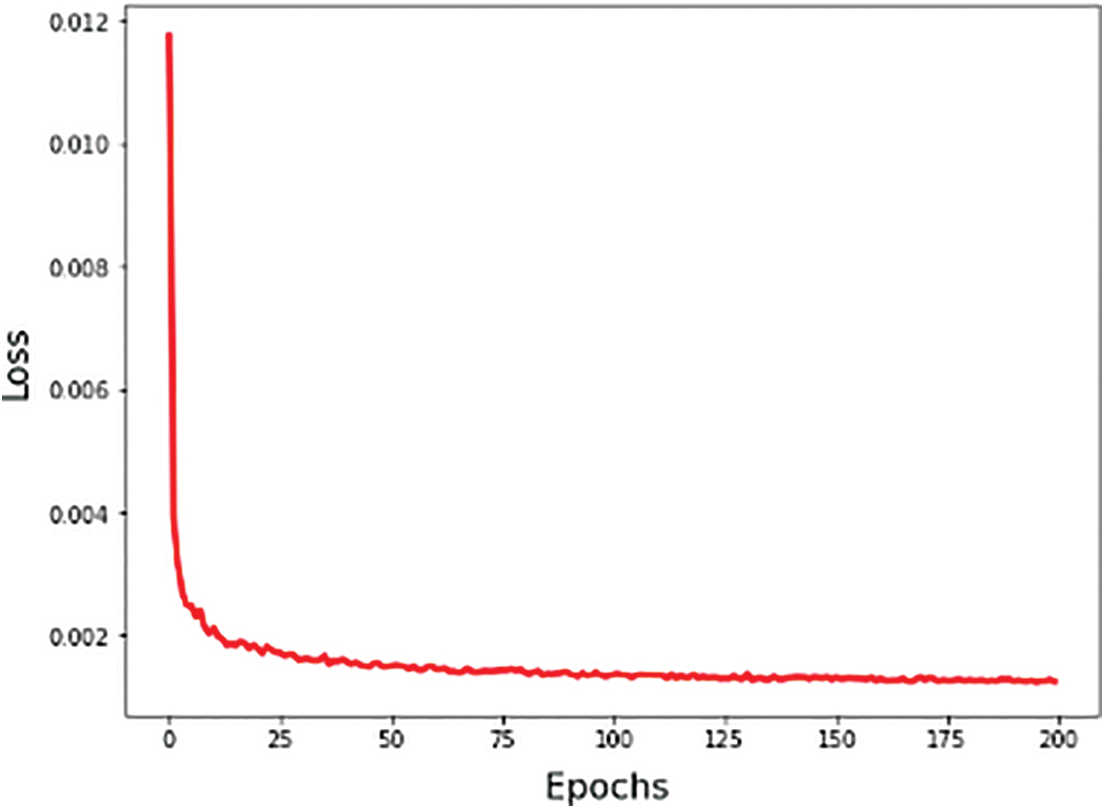
Figure 8: Loss curve

Fig. 9 presents a representation of our model forecasting results on the household power dataset.

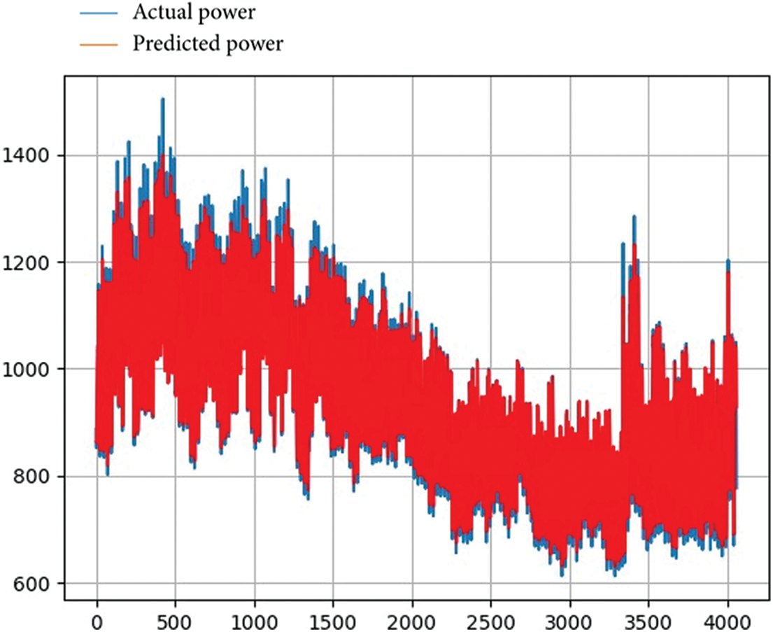
Figure 9: Forecasting energy using LSTM-DELM

5  Conclusions

Deep learning models demonstrated their potent learning and prediction capabilities in time series prediction. We recommend the use of hybrid deep learning models, especially LSTM-DELM models to predict energy consumption in the case of smart building. Focusing on the objective of this research, a new model was proposed in order to predict energy in houses. It’s a hybrid approach that combines LSTM with DELM (with seven hidden layers). It was successfully compared in terms of its prediction performance with other statistical models The consequence of the model training and testing shows that our model has shown its strength in predicting energy consumption in terms of MAE (0.42), R-squared (1, 1) and RMSE (1.23). The model proposed with a modified architecture of DELM outperforms other models. It can be applicable in multiple IoT applications such as smart cities, smart homes, smart buildings and smart grids.

Acknowledgement: This work is part of a Tunisian-South African cooperation scientific research project. We thank the Ministry of Higher Education and Scientific Research of Tunisia that has supported this research.

Funding Statement: The authors received no funding for this study.

Conflicts of Interest: The authors declare that they have no conflicts of interest to report regarding the present study.

References

1. A. Vishwanath, V. Chandan and K. Saurav, “An IoT-based data driven precooling solution for electricity cost savings in commercial buildings,” IEEE Internet of Things Journal, vol. 6, no. 5, pp. 7337–7347, 2019. [Google Scholar]

2. J. Huang, “Energy efficiency improvement of composite energy building energy supply system based on multiobjective network sensor optimization,” Journal of Sensors, vol. 2022, 2022. [Google Scholar]

3. D. B. Crawley, L. K. Lawrie, F. C. Winkelmann, W. F. Buhl, Y. J. Huang, et al., “EnergyPlus: Creating a new-generation building energy simulation program,” Energy and Buildings, vol. 33, no. 4, pp. 319–331, 2001. [Google Scholar]

4. D. Yan, J. Xia, W. Tang, F. Song, X. Zhang et al.,“DeST—An integrated building simulation toolkit part I: Fundamentals,” Building Simulation, vol. 1, no. 2, pp. 95–110, 2008. [Google Scholar]

5. Zhu, Y., “Applying computer-based simulation to energy auditing: A case study,” Energy and Buildings, vol. 38, no. 5, pp. 421–428, 2006. [Google Scholar]

6. J. Seo, S. Kim, S. Lee, H. Jeong, T. Kim et al., “Data-driven approach to predicting the energy performance of residential buildings using minimal input data,” Building and Environment, vol. 214, pp. 108911, 2022. [Google Scholar]

7. C. Nakkach, A. Zrelli and T. Ezzdine, “Deep learning algorithms enabling event edtection: A review,” in the 2nd Int. Conf. on Industry 4.0 and Artificial Intelligence (ICIAI 2021), Tunisia, Sousse, pp. 170–175, 2022. [Google Scholar]

8. K. Mirzaei, M. Arashpour, E. Asadi, H. Masoumi, Y. Bai et al., “3D point cloud data processing with machine learning for construction and infrastructure applications: A comprehensive review,” Advanced Engineering Informatics, vol. 51, pp. 101501, 2022. [Google Scholar]

9. C. Nakkach, A. Zrelli and T. Ezzedine, “Smart border surveillance system based on deep learning methods,” in the Int. Symp. on Networks, Computers and Communications (ISNCC), Shenzhen, China, pp. 1–6, 2022. [Google Scholar]

10. A. Zrelli, C. Nakkach and T. Ezzedine, “Cyber-security for IoT applications based on ANN algorithm,” in Int. Symp. on Networks, Computers and Communications (ISNCC), Shenzhen, China, pp. 1–5, 2022. [Google Scholar]

11. C. Nakkach, A. Zrelli and T. Ezzedine, “Plane’s detection in border area using modern deep learning methods,” in the IEEE/ACIS 22nd Int. Conf. on Computer and Information Science (ICIS), Zhuhai, China, pp. 88–93, 2022. [Google Scholar]

12. V. Jasti, A. S. Zamani, K. Arumugam, M. Naved, H. Pallathadka et al., “Computational technique based on machine learning and image processing for medical image analysis of breast cancer diagnosis,” Security and Communication Networks, vol. 2022, 2022. [Google Scholar]

13. Y. Duan, J. W. Goodell, H. Li and X. Li, “Assessing machine learning for forecasting economic risk: Evidence from an expanded Chinese financial information set,” Finance Research Letters, vol. 46, pp. 102273, 2022. [Google Scholar]

14. C. Nakkach, A. Zrelli and T. Ezzdine, “An efficient approach of vehicle vetection based on deep learning algorithms and wireless sensors networks,” International Journal of Software Innovation (IJSI), vol. 10, no. 1, pp. 1–16, 2022. [Google Scholar]

15. A. S. Shah, H. Nasir, M. Fayaz, A. Lajis and A. Shah, “A review on energy consumption optimization techniques in IoT based smart building environments,” Information, vol. 10, no no. 3, pp. 108, 2019. [Google Scholar]

16. M. Castelli, L. Trujillo, L. Vanneschi and A. Popovič, “Prediction of energy performance of residential buildings: A genetic programming approach,” Energy and Buildings, vol. 102, pp. 67–74, 2015. [Google Scholar]

17. K. Li, X. Xie, W. Xue, X. Dai, X. Chen et al., “A hybrid teaching-learning artificial neural network for building electrical energy consumption prediction,” Energy and Buildings, vol. 174, pp. 323–334, 2018. [Google Scholar]

18. F. Wahid and D. H. Kim, “Short-term energy consumption prediction in Korean residential buildings using optimized multi-layer perceptron,” Kuwait Journal of Science, vol. 44, no. 2, pp. 67–77, 2017. [Google Scholar]

19. M. Collotta and G. Pau, “An innovative approach for forecasting of energy requirements to improve a smart home management system based on BLE,” IEEE Transactions on Green Communications and Networking, vol. 1, no. 1, pp. 112–120, 2017. [Google Scholar]

20. S. Sholahudin and H. Han, “Simplified dynamic neural network model to predict heating load of a building using taguchi method,” Energy, vol. 115, pp. 1672–1678, 2016. [Google Scholar]

21. D. Zhao, M. Zhong, X. Zhang and X. Su, “Energy consumption predicting model of VRV (Variable refrigerant volume) system in office buildings based on data mining,” Energy, vol. 102, pp. 660–668, 2016. [Google Scholar]

22. S. Goudarzi, M. H. Anisi, N. Kama, F. Doctor, S. A. Soleymani et al., “Predictive modelling of building energy consumption based on a hybrid nature-inspired optimization algorithm,” Energy and Buildings, vol. 196, pp. 83–93, 2019. [Google Scholar]

23. Y. H. Lin and Y. C. Hu, “Electrical energy management based on a hybrid artificial neural network-particle swarm optimization-integrated two-stage non-intrusive load monitoring process in smart homes,” Processes, vol. 6, no. 12, pp. 236, 2018. [Google Scholar]

24. S. Naji, A. Keivani, S. Shamshirband, U. J. Alengaram, M. Z. Jumaat et al., “Estimating building energy consumption using extreme learning machine method,” Energy, vol. 97, pp. 506–516, 2016. [Google Scholar]

25. M. Fayaz and D. Kim, “Energy consumption optimization and user comfort management in residential buildings using a bat algorithm and fuzzy logic,” Energies, vol. 11, no. 1, pp. 161, 2018. [Google Scholar]

26. S. S. Subbiah, S. K. Paramasivan, K. Arockiasamy, S. Senthivel and M. Thangavel, “Deep learning for wind speed forecasting using bi-lstm with selected features,” Intelligent Automation & Soft Computing, vol. 35, no. 3, pp. 3829–3844, 2023. [Google Scholar]

27. S. Salcedo-Sanz, L. Cornejo-Bueno, L. Prieto, D. Paredes and R. García-Herrera, “Feature selection in machine learning prediction systems for renewable energy applications,” Renewable and Sustainable Energy Reviews, vol. 90, pp. 728–741, 2018. [Google Scholar]

28. J. Cheng, Z. Duan and Y. Xiong, “QAPSO-BP algorithm and its application in vibration fault diagnosis for a hydroelectric generating unit,” J. Vib. Shock, vol. 34, no. 23, pp. 177–181, 2015. [Google Scholar]

29. S. Ding, N. Zhang, X. Xu, L. Guo and J. Zhang, “Deep extreme learning machine and its application in EEG classification,” Mathematical Problems in Engineering, vol. 2015, 2015. [Google Scholar]

30. D. Xiao, B. Li and Y. Mao, “A multiple hidden layers extreme learning machine method and its application,” Mathematical Problems in Engineering, vol. 2017, 2017. [Google Scholar]

31. G. B. Huang, Q. Y. Zhu and C. K. Siew, “Extreme learning machine: Theory and applications,” Neurocomputing, vol. 70, no. 1–3, pp. 489–501, 2006. [Google Scholar]

32. G. Hebrail and A. Berard, “Individual household electric power consumption data set,” in: É. d. France(Ed.UCI Machine Learning Repository, 2012. [Google Scholar]