Online Markov Blanket Learning with Group Structure

1  Introduction

The Markov blanket (MB) is an essential substructure in the Bayesian network (BN). Under the faithfulness assumption, the MB of a given variable is unique and consists of parents (direct causes), children (direct effects), and spouses (the other parents of the children) of the variable, which represents the local causal relationships of the variable [1]. Since a given variable is independent of others conditioning on its MB, the MB of the variable is the optimal feature subset [2–4]. Identifying MB of a given variable captures the causal relationship between the variable and selected variables, enhancing the interpretability of the prediction model [5,6].

Standard MB learning algorithms must obtain the entire variable space [7–10]. However, not all variables can be obtained in advance [11]. Online MB learning algorithms have recently received more and more attention because they can dynamically process variables [12,13]. Nevertheless, in application scenarios, features are generated in groups [14]. For example, in environmental monitoring and analysis, researchers will deploy monitoring stations at different locations, and each station will continuously generate data [15]; in medical examination, the different inspection items will generate different feature groups [16–18]. In such application scenarios with group features arrived, if directly using the existing online MB learning algorithm, group features need to be split into one by one feature, which will destroy the original group structure, leading to loss of information and reduced accuracy.

Motivated by this, we focus on online MB learning with group structure, and the contributions of this paper are as follows:

i)   Different from online MB learning, we address the problem of online group MB learning instead of online individual MB learning. To the best of our knowledge, this is the first effort considering the online group MB learning problem.

ii)   We propose OMBGS, Online MB learning with Group Structure, which consists of two parts: intra-group selection and inter-group selection. OMBGS first selects MB of a class variable within the newly arrived feature group, and then selects MB of the class variable under the current feature space.

iii)   We conducted experiments on eight benchmark BN datasets to validate the accuracy of the proposed algorithms by comparison with eight standard MB learning algorithms and three online MB learning algorithms.

The remainder of this paper is organized as follows. In Section 2, we review the related work. In Section 3, we describe the basic notations and definitions. In Section 4, we provide the proposed algorithms in detail, and in Section 5, we discuss the experimental results and their interpretation. Finally, Section 6 concludes this paper.

2  Related Work

In this section, we first discuss the standard MB learning algorithms, then review the Online MB learning algorithms.

2.1 Standard Markov Blanket Learning

Standard MB learning algorithms are divided into simultaneous and divide-and-conquer algorithms [9]. Simultaneous algorithms are efficient, but the accuracy may suffer when the sample size is insufficient because it uses a large conditioning set, and conditional independence tests are less accurate with a large conditioning set [19,20]. Divide-and-conquer algorithms improve the accuracy of the simultaneous algorithms with small samples by reducing the size of the conditioning set, and dividing it into two steps: parents and children (PC) learning and spouses learning.

Incremental Association MB (IAMB) [21] is a typical representative of simultaneous algorithms. IAMB first discovers all possible MB of a given variable conditioning on the selected MB, then removes all false-positives. Later, multiple variants of IAMB were proposed (e.g., FBED [22] and EAMB [23]).

Min-max MB (MMMB) [24] algorithm is the earliest divide-and-conquer algorithm. MMMB first uses a subset of the currently selected PC to identify the PC of a given variable, and then uses the obtained PC to identify spouses of the variable. Later, HITONMB [25] improved the efficiency of MMMB via the interleaved addition and removal of parent or child. To improve the efficiency of previous algorithms, simultaneous MB (STMB) [26] identifies all spouses from non-PC of a given variable. However, STMB algorithm uses a larger conditioning set in the spouses learning phase, which reduces the accuracy of learning the MB of a given variable. Balanced MB discovery (BAMB) [27] and the efficient and effective MB discovery (EEMB) [28] reduce the size of the conditioning set of STMB in the spouses learning phase, which improves the accuracy of STMB with small samples. Cross-check and complement MB discovery (CCMB) [29] reduces the impact of conditional independence test errors on MB learning through OR rules. Causal Feature Selection framework (CFS) [30] improves the efficiency of MB learning algorithms by reducing the skeleton structure to be expanded during spouses learning.

2.2 Online Markov Blanket Learning

Online MB learning algorithms can learn MB for a given variable without acquiring the entire variable space. Online causal feature selection for streaming features (OCFSSF) [12] algorithm is the earliest proposed online MB learning algorithm. When a new variable arrives, OCFSSF algorithm can dynamically determine whether the current variable is the MB node of the target variable. However, OCFSSF algorithm cannot remove all false-positive spouses. Online simultaneous MB learning (O-ST) [13] algorithm takes the currently selected MB as the condition set and obtains the MB in the current state on the fly. Online divide-and-conquer MB learning (O-DC) [13] algorithm is based on mutual information theory. After a new variable has arrived, O-DC identifies PC and spouses of a given variable in the current state.

However, the existing online MB learning algorithms can not handle features with the group structure because online MB learning algorithms can only process a single feature at a time. To tackle these problems, in this paper, we propose online MB learning with group structure algorithm to accurately identify the MB of a given variable.

3  Notations and Definitions

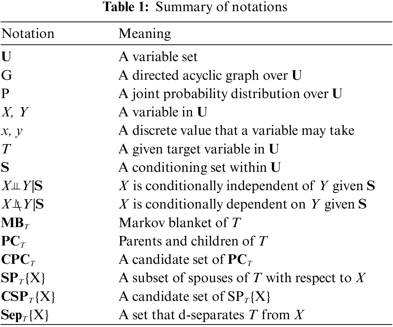
In this section, we describe basic definitions and theorems. Table 1 summarizes the notations used in this paper.

Definition 1 (Bayesian Network) [31]. A triplet <U, G, P> is called a Bayesian network iff <U, G, P> satisfies the Markov condition: each variable in U is independent of all non-descendants of the variable conditioning on its parents.

Definition 2 (Faithfulness) [32]. A BN <U, G, P> is faithful iff all conditional dependencies between features in G are captured by P.

Definition 3 (Conditional Independence) [30]. For two variables X and Y are conditionally independent given a set S (i.e., X⫫Y|S), if P(X = x, Y = y|S = s) = P(X = x|S = s) P(Y = y|S = s).

Definition 4 (D-separation) [31]. For two variables X and Y are conditionally independent given S (S ⊆ U\{X ∪ Y}), iff each path from X to Y is blocked by the set S. For a path π between X and Y, if a collider and it descendants on π is not included in S, or every non-collider on π is included in S, then path π is blocked by S.

Under the faithfulness assumption, Definition 4 can be used to determine whether two variables are independent given a conditioning set.

Definition 5 (Markov Blanket) [31]. In a faithful BN, MB of each variable is unique and consists of its parents, children, and spouses (the other parents of its children).

Given MB of T, MBT, all other variables are conditionally independent of T, that is, Y⫫T|MBT, for $∀ Y∈ U\MBT\T. Thus, MB is the optimal feature subset for prediction.

Definition 6 (V-Structure) [31]. Three variables T, X, Y form a V-structure (i.e., T → X ← Y), iff T and Y are both parents of X.

The V-structure can be used to identify spouses of a given variable. Such as, if there is a V-structure T → X ← Y, then Y is a spouse of T.

Theorem 1 [31–33]. In a faithful BN, given two variables T ∈ U and X ∈ U, if there is an edge between T and X, then TX|S, for ∀ S ⊆ U\{T, X}.

4  Proposed Algorithm

In this section, we first describe the OMBGS algorithm, then describe two of the important subprograms, and finally analyze the correctness of the OMBGS algorithm.

4.1 The OMBGS Algorithm

In this subsection, we propose the OMBGS, and the pseudo-code of the OMBGS is shown in Algorithm 1, which consists of two parts: intra-group selection and inter-group selection. For the newly arrived variable group, OMBGS first identifies the MB of a given variable within the newly arrived group (Lines 4–10), and then obtains the MB of the variable in the current variable space via the newly arrived group (Lines 11–25).

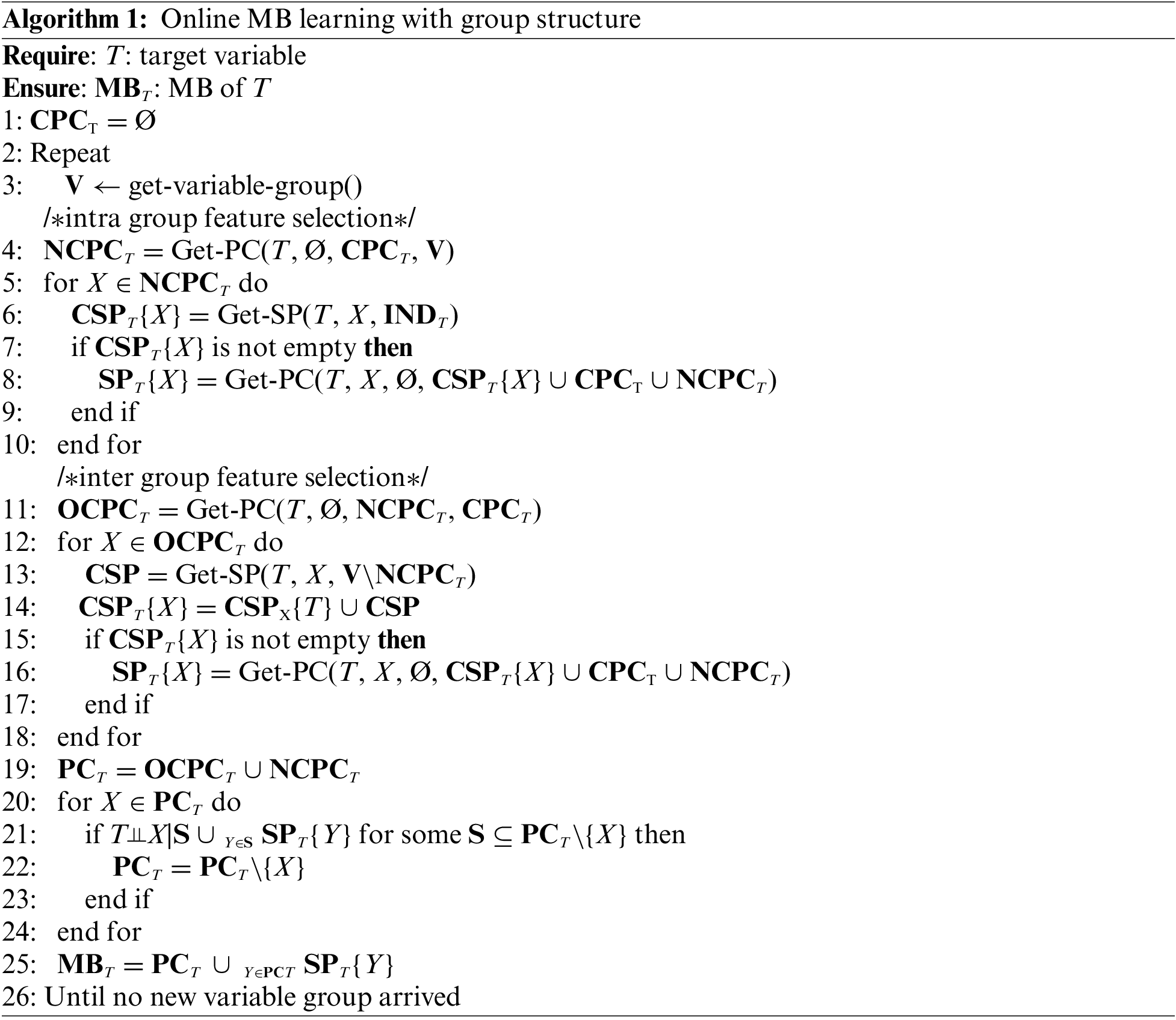
The Part 1 in OMBGS (Algorithm 1, Lines 4–10) identifies the MB of a class variable from the newly arrived variable group. OMBGS first uses Get-PC (Algorithm 2) to identify the PC of the class variable from the newly arrived variable group V (Line 4). Then, based on the identification of PC (NCPCT) from the newly arrived variable group, OMBGS identifies spouses with respect to these PC (Lines 5–10). For a newly identified PC, X, OMBGS uses Get-SP (Algorithm 3) to identify all possible spouses from variables that are independent of the class variable (INDT) in the current feature space (Line 6). If the spouses can be identified by variable X, then continue to remove all false-positives in the identified spouses (Lines 7–9).

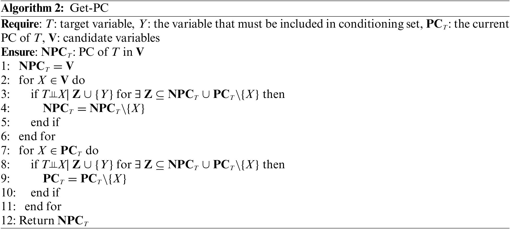
Note that the Get-PC subroutine utilizes Theorem 1 to identify PC of a class variable, and the essence of Get-PC is to identify all variables that are independent of a class variable. Thus, according to Definition 6, we can use Get-PC to remove variables independent of the class variable in a containing set that includes X for learning all true-positive spouses.

The Part 2 in OMBGS (Algorithm 1, Lines 11–25) identifies the MB of a class variable under the current variable space. OMBGS first uses Get-PC to remove false-positives in CPCT based on newly identified NCPCT (Line 11). Then, similar to Part 1, OMBGS identifies spouses of the class variable from the newly arrived variable group V according to the variables in OCPCT (Lines 12–18). Finally, OMBGS uses the currently identified MB to remove the false-positives in PCT (Lines 20–25).

4.2 The Get-PC Subroutine

Based on the PC of a target variable T in the current state, PCT (initially, PCT is the empty set). OMBGS first uses the currently identified PC, PCT, to identify the false-positive PC in the newly arrived variable group for minimizing the current candidate PC (Lines 2–6). Then, using the newly identified PC, NPCT, OMBGS removes the false positives in PCT (Lines 7–11).

Proposition 1. Any true-positive PC in V is included in the identified NPCT.

Proof: For each variable in V, the algorithm Get-PC uses a subset of the currently selected PC (PCT) as the condition set to determine whether it is independent of the class variable. According to Theorem 1, the PC of a class variable is strongly correlated features, and the nodes independent of the class variable for the current condition must be non-PC of the class variable.

4.3 The Get-SP Subroutine

Proposition 2. In a faithful BN, for a variable T, if variable X is a spouse of T with respect to Y, then T and X are dependent containing on a set including Y.

Proof: For a variable T, if variable X is a spouse of T with respect to X, there exists the structure, T → Y ← X, where variable Y is a collider. According to D-separation, we can obtain that T and X are conditionally dependent when Y is in the conditioning set, because the path T-Y-X between T and X is open. Thus, the conditioning set includes PC of T, Y, and T and X are conditionally independent.

For each variable in V (Line 2), the Get-SP subroutine determines whether the variable is a spouse of a given variable T (Lines 3–5). According to Proposition 2, the Get-SP subroutine identifies all spouses (CSPT{Y}) of the given variable T with respect to a variable Y.

4.4 Correctness of OMBGS

Proposition 3. Under the faithfulness assumption, OMBGS finds the correct MB of a class variable under the current feature space.

Proof: First, we show that OMBGS can discover all PC and spouses of a class variable. For PC discovery, OMBGS uses Get-PC (Algorithm 2) to discover the PC of a class variable T in the newly arrived feature group V. All PC will be discovered owing to Proposition 1. For spouses discovery, OMBGS first obtains spouses from INDT by newly joining PC, NCPCT (Line 6), and then obtains spouses from the newly arrived feature group by OCPCT (Line 13). After these two steps, all spouses will be discovered owing to Proposition 2. Second, we show that OMBGS will remove all false-positive spouses and PC. For the false-positives in CSPT{X}, OMBGS use CSPT{X} ∪ CPCT ∪ NCPCT to remove them (Line 8). Since this step will remove all variables independent of T about X. Thus, all false-positive spouses are removed. For the PC in the current state, OMBGS first removes the false-positives from them using the newly identified PC (Line 11), and then based on the property of MB, OMBGS removes all false-positive PC using the current MB (Line 20–25). Thus, all false-positive PC in the current state will be removed.

4.5 Computational Complexity

We use the number of conditional independence tests to represent the time complexity of OMBGS algorithm. Assume that |N| denotes the number of all arrived variables in the current state and |V| denotes the number of feature groups that arrive in the next state. In the intra-group selection phase, for PC learning, Algorithm 2 uses the subsets of the union of currently selected PC and feature group V to identify PC of a given variable in V, and the time complexity is O(|V|2|PC|+|V|). For spouses learning, for each variable in the newly identified PC, the possible spouses are identified from the non-PC of the given variable, and the time complexity is O(|PC||nonPC|), and the true-positive spouses are identified by removing all false spouses, and the time complexity is O(|PC||CSP|2|CSP|+|PC|). Similarly, in the inter-group selection phase, for PC learning, the time complexity is O(|PC|2|PC|), and for spouses learning, the time complexity is O(|PC||nonPC|) + O(|PC||CSP|2|CSP|+|PC|). Thus, the time complexity of OMBGS is O(|PC||CSP|2|CSP|+|PC|).

5  Experiments

In this section, we evaluate the proposed OMBGS. We first describe datasets, compared algorithms, and evaluate metrics used in the experiment. Then we summarize and discuss the experimental results.

5.1 Experiment Setting

5.1.1 Datasets

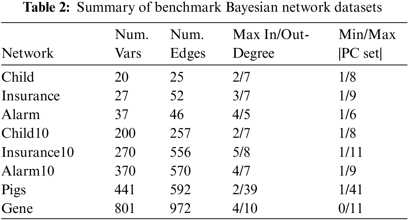
Table 2 shows the eight benchmark BN datasets (Child, Insurance, Alarm, Child10, Insurance10, Alarm10, Pigs, and Gene). We used two data groups for each benchmark BN network, one contained ten datasets with 500 data samples, and the other contained ten datasets with 5000 data samples. The number of variables in these datasets ranges from 20 to 801.

5.1.2 Comparison Algorithms

We compare the proposed algorithm OMBGS against the following eight standard MB learning algorithms and three online MB learning algorithms:

Standard MB learning algorithms

1) MMMB [24]. MMMB algorithm first uses MMPC [24] algorithm to learn PC of a given variable, and then learns PC of each variable in PC of the given variable for obtaining spouses of the given variable.

2) HITONMB [25]. Compared to MMMB, HITONMB uses HITONPC [25] for learning the PC of a given variable.

3) STMB [26]. STMB algorithm first uses PCsimple [26] to learn the PC of a given variable, and then identifies spouses from non-PC of the given variable.

4) BAMB [27]. BAMB algorithm uses HITONPC to add and remove PC and spouses of a given variable alternately.

5) EEMB [28]. EEMB algorithm first uses HITONPC to learn PC and spouses of a given variable alternately, then removes false-positives.

6) CCMB [29]. CCMB algorithm finds the PCMasking phenomenon caused by the conditional independence test error and avoids the error using symmetry checking.

7) CFS [30]. CFS algorithm reduces the skeleton structure that needs to be expanded when identifying spouses by identifying the children with multiple parents (C-MP) in the PC of a class variable.

8) EAMB [23]. EAMB algorithm recovers missed true-positive MB from the removed MB to avoid false deletes due to conditional independence test errors.

Online MB learning algorithms

1) OCFSSF [12]. OCFSSF algorithm alternately learns the PC and spouses of a class variable via the newly arrived variable to obtain the MB of the class variable on the fly.

2) O-ST [13]. O-ST algorithm uses the property of MB to determine whether a newly arrived variable is an MB of a class variable on the fly.

3) O-DC [13]. O-DC algorithm based on mutual information theory to identify MB of a class variable via the new arrival feature on the fly.

5.1.3 Evaluation Metrics

MATLAB was used to implement all the algorithms. Standard MB learning algorithms are implemented by Causal learner [34]. All experiments were conducted on a Windows 10 computer with an Intel Core i7-4790 processor and 16 GB of RAM. The best results are shown in bold in the tables in the experimental results.

We run every algorithm for each variable in every network. On the benchmark BN datasets, the following metrics were used to assess the algorithms:

Precision: Precision is the number of true-positives in the output (i.e., variables in the output that belong to the MB of a given variable) divided by the number of variables in the output of an algorithm.

Recall: Recall represents the number of true-positives in the output divided by the number of true-positives (i.e., the amount of the MB of a given variable).

F1: F1 is the harmonic average of Precision and Recall (F1 = 2 * precision * recall/(precision + recall)), where F1 = 1 is the best case, and F1 = 0 is the worst case.

Time: Time is the runtime of an algorithm.

We report the average F1, precision, recall, and runtime for ten datasets for each algorithm. The results are presented in the following tables in the format A ± B, where A denotes the average F1, Precision, Recall, or Time, and B denotes the standard deviation.

5.2 Experiment Result

5.2.1 OMBGS and Standard MB Learning Algorithms

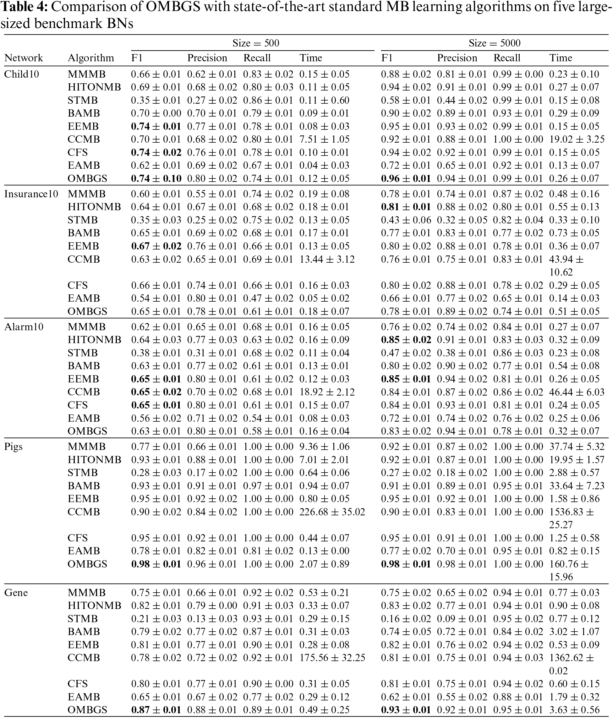
We compare OMBGS with MMMB, HITONMB, STMB, BAMB, EEMB, CCMB, CFS, and EAMB on the eight BNs, as shown in Table 2. The average results of F1, Precision, Recall, and Time of each algorithm are reported in Tables 3 and 4. Table 3 summarizes the experimental results on three small-sized BN datasets (Child, Insurance, and Alarm), and Table 4 reports the experimental results on five large-sized BN datasets (Child10, Insurance10, Alarm10, Pigs, and Gene). Since the benchmark BN datasets do not have a group structure, we divided the dataset into ten groups according to the order of the variable number as the input of OMBGS algorithm. Since OMBGS and standard MB algorithms process different data types, we only compare the accuracy (F1) rather than the efficiency of OMBGS and its rivals. From the experimental results, we have the following observations.

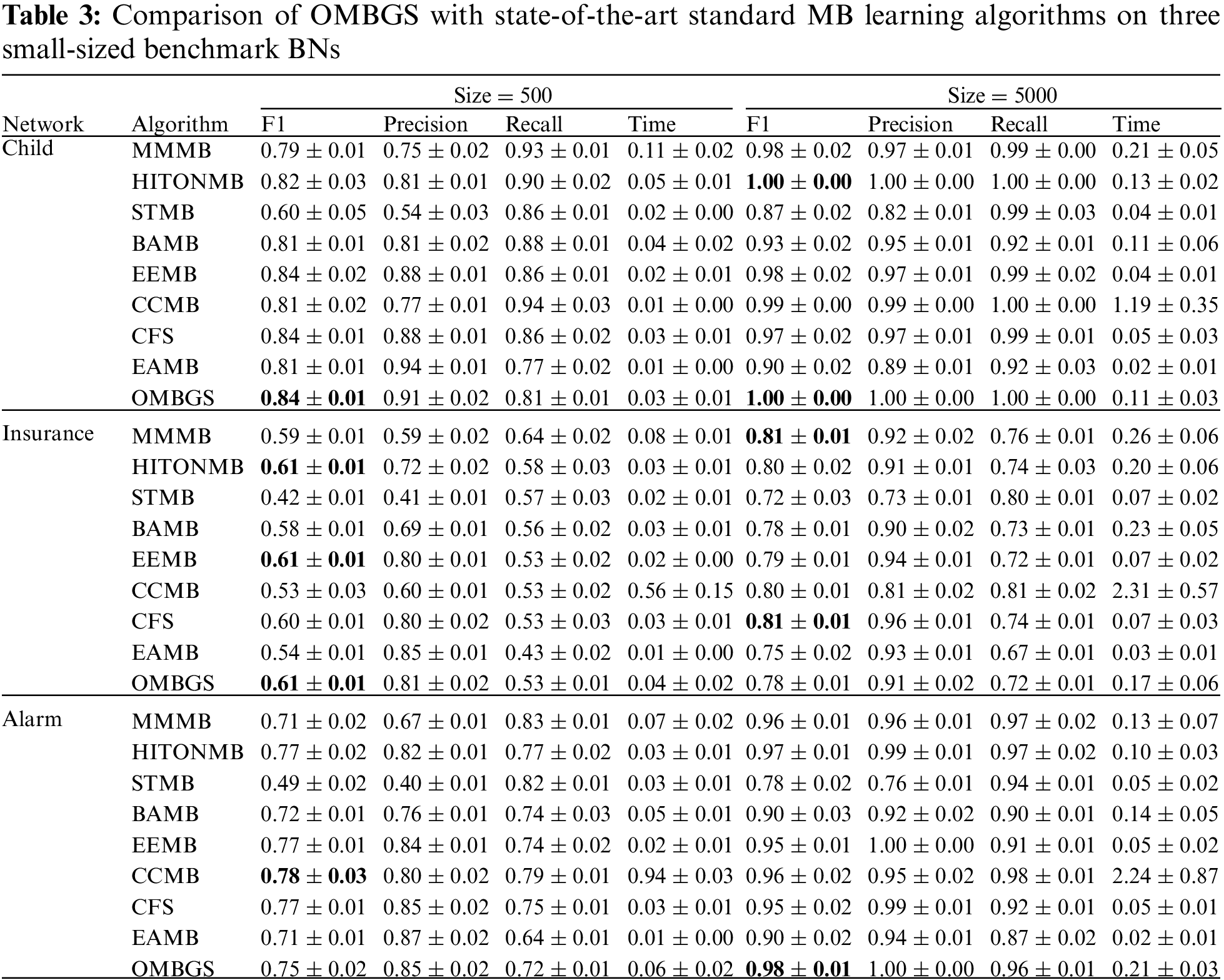
On the Child network, regardless of the number of samples, OMBGS is the most accurate in terms of F1 metric compared to other algorithms. On the Insurance network with 500 samples, OMBGS is more accurate than its rivals. However, on the Insurance network with 5000 samples, compared with standard MB learning algorithms, OMBGS does not achieve a high accuracy, which may be due to some information missing due to grouping, and thus the true-positives are removed. On the Alarm network with 500 samples, OMBGS achieves higher accuracy than half of the comparison algorithms. On the Alarm network with 5000 samples, OMBGS algorithm achieves higher accuracy than all comparison algorithms.

Compared to other algorithms, OMBGS achieved the highest accuracy on three out of five datasets on large-sized networks. Especially on the high-dimensional Pigs and Gene datasets, OMBGS has more than 3% and 6% improvement in accuracy compared to other algorithms. It shows that OMBGS can be better applied to high-dimensional data than the standard MB learning algorithms.

To make a more intuitive comparison, the accuracy (using F1 metric) of OMBGS with its rivals is shown in Fig. 1. As we can see from the figure, OMBGS has comparable accuracy to the standard MB learning algorithms on all datasets. In particular, on the high-dimensional datasets Pigs and Gene, OMBGS has a significant advantage over its rivals.

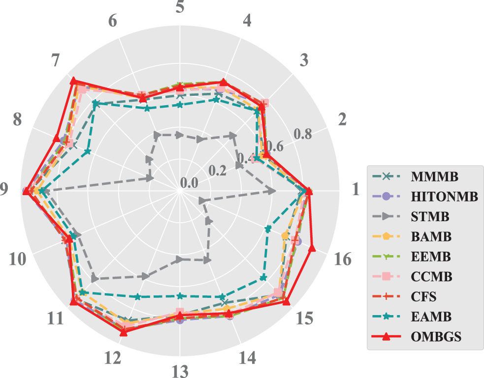
Figure 1: The accuracy results of the experiments (the higher the F1 value is, the better the result) of OMBGS and standard MB learning algorithms on eight benchmark BN datasets with 500 samples and 5000 samples. (Numbers 1 to 8 denote the datasets with 500 samples: 1: Child, 2: Insurance, 3: Alarm, 4: Child10, 5: Insurance10, 6: Alarm10, 7: Pig, 8: Gene. Numbers 9 to 16 denote the datasets with 5000 samples: 9: Child, 10: Insurance, 11: Alarm, 12: Child10, 13: Insurance10, 14: Alarm10, 15: Pig, 16: Gene)

Meanwhile, to further evaluate OMBGS against its rivals, we performed the Friedman test at the 5% significance level. For accuracy, the null hypothesis of MMMB, HITONMB, STMB, BAMB, EEMB, CCMB, CFS, EAMB, and OMBGS is rejected, and the average ranks are 3.88, 6.88, 1.06, 4.25, 7.25, 5.22, 6.81, 2.38, and 7.28, respectively. Then, we proceed with the Nemenyi test as a post hoc test. In the Nemenyi test, with a critical difference of 3.00, OMBGS was significantly faster than its rivals, and the crucial difference diagram of the Nemenyi test is shown in Fig. 2.

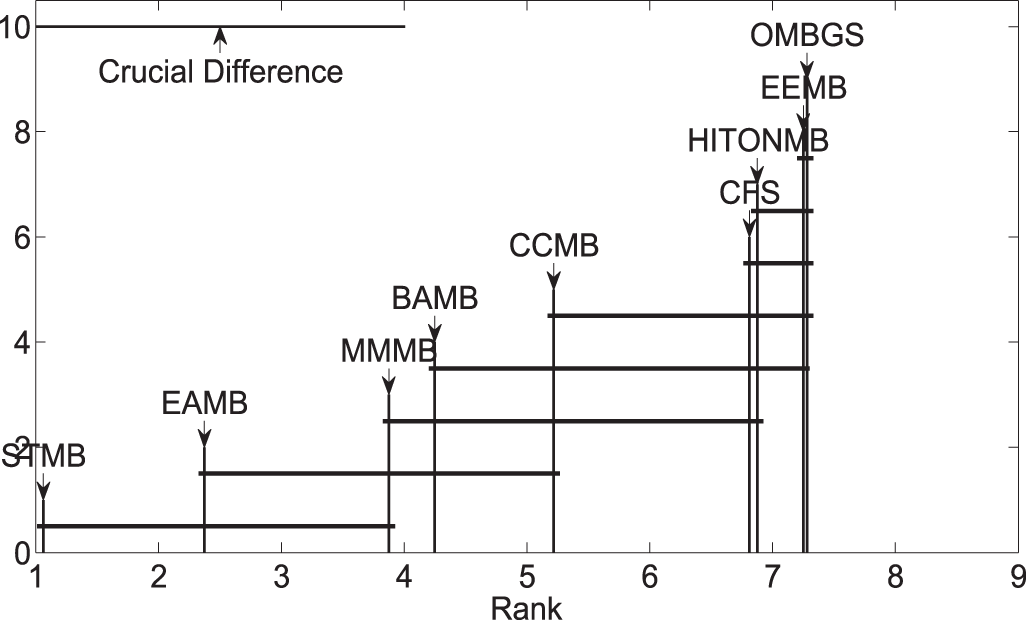
Figure 2: Crucial difference diagram of the Nemenyi test for the accuracy of OMBGS and standard MB learning algorithms

5.2.2 OMBGS and Online MB Learning Algorithms

We compare OMBGS with OCFSSF, O-ST, and O-DC on the eight BN datasets, as shown in Table 5. The average results of F1, Precision, Recall, and running time of each algorithm are reported in Table 5. For online MB learning algorithms, we add variables in variable numbers order. From the experimental results, we have the following observations.

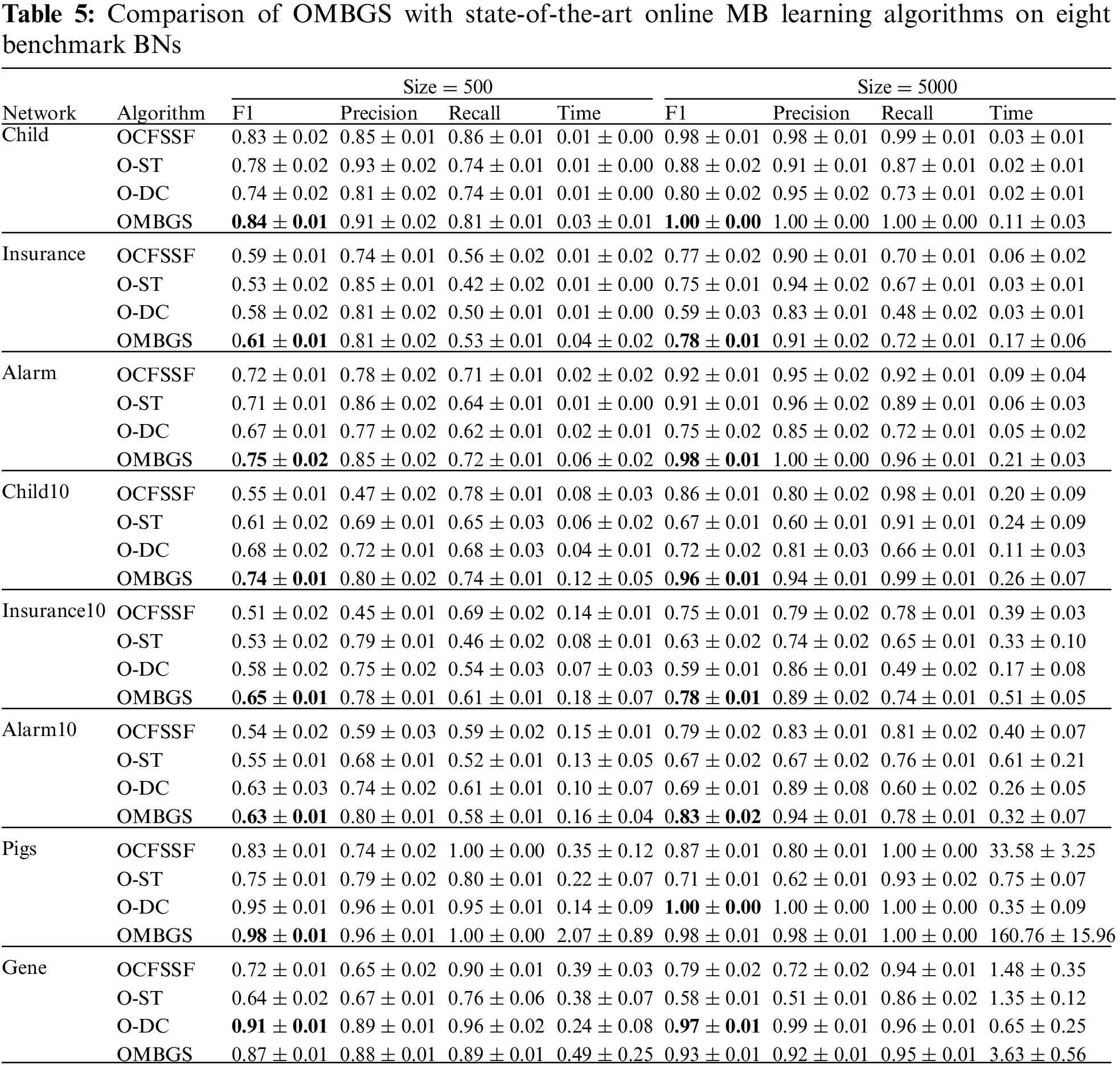
The OMBGS algorithm significantly outperforms the OCFSSF and O-ST algorithms on all datasets, and the OMBGS algorithm outperforms the O-DC algorithm on 13 out of 16 datasets. This shows that the online group MB learning algorithm has a significant advantage over the online MB learning algorithm. On the Gene dataset, OMBGS outperforms OCFSSF and O-ST, which also use conditional independence tests, but is slightly worse than the O-DC algorithm, which uses mutual information, and thus applying mutual information for PC learning may be a future research direction to improve the accuracy of online group MB learning. Online MB learning algorithms achieve less running time because some of the correct variables are removed in advance, thus its accuracy is significantly lower than that of OMBGS.

To make a more intuitive comparison, the accuracy (using F1 metric) of OMBGS with its rivals is shown in Fig. 3. As we can see from the figure, OMBGS significantly outperforms its rivals on most data sets. Meanwhile, to further evaluate OMBGS against its rivals, we performed the Friedman test at the 5% significance level. For accuracy, the null hypothesis of OCFSSF, O-ST, O-DC, and OMBGS is rejected, and the average ranks are 2.38, 1.56, 2.28, and 3.78, respectively. Then, we proceed with the Nemenyi test as a post hoc test. In the Nemenyi test, with a critical difference of 1.17, OMBGS was significantly faster than its rivals, and the crucial difference diagram of the Nemenyi test is shown in Fig. 4.

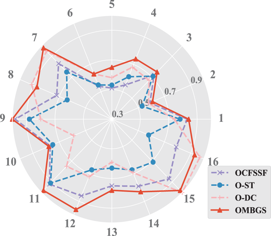
Figure 3: The results of the experiments on the accuracy of OMBGS and online MB learning algorithms on eight benchmark BN datasets with 500 samples and 5000 samples (The numbers 1 to 16 are the same as those in Fig. 1)

Figure 4: Crucial difference diagram of the Nemenyi test for the accuracy of OMBGS and online MB learning algorithms

6  Conclusion

In this paper, we propose an OMBGS algorithm to address the problem of online group MB learning. OMBGS consists of two parts, intra-group and inter-group selection, which are used to identify the MB of the new arrival variable group and the current variable space, respectively. Experiments conducted on eight BN datasets indicated the effectiveness of the proposed algorithm. However, the proposed OMBGS algorithm depends on the conditional independence test, and the accuracy of the conditional independence test is lower when the data sample is small. Thus, future research could focus on proposing new methods for online MB discovery with group structure without using conditional independence tests.

Funding Statement: This work was supported by the National Natural Science Foundation of China [No. 62272001, No. U1936220, No. 61872002, No. 61876206 and No. 62006003]. The National Key Research and Development Program of China [No. 2019YFB1704101], the Natural Science Foundation of Anhui Province of China [No. 2108085QF270].

Conflicts of Interest: The authors declare that they have no conflicts of interest to report regarding the present study.

References

1. J. Pearl, Probabilistic Reasoning in Intelligent Systems. Amsterdam, Netherlands: Elsevier, 2014. [Google Scholar]

2. L. Shi, P. Lu and J. Yan, “Causality learning from time series data for the industrial finance analysis via the multi-dimensional point process,” Intelligent Automation & Soft Computing, vol. 26, no. 5, pp. 873–885, 2020. [Google Scholar]

3. Y. Sreeraman and S. L. Pandian, “Design and experimentation of causal relationship discovery among features of healthcare datasets,” Intelligent Automation & Soft Computing, vol. 29, no. 2, pp. 539–557, 2021. [Google Scholar]

4. K. Yu, L. Liu and J. Li, “A unified view of causal and non-causal feature selection,” ACM Transactions on Knowledge Discovery from Data (TKDD), vol. 15, no. 4, pp. 1–46, 2021. [Google Scholar]

5. X. Wu, B. Jiang, K. Yu, H. Chen and C. Miao, “Multi-label causal feature selection,” Proc. of the AAAI Conf. on Artificial Intelligence, vol. 34, no. 4, pp. 6430–6437, 2020. [Google Scholar]

6. X. Wu, B. Jiang, Y. Zhong and H. Chen, “Multi-target Markov boundary discovery: Theory, algorithm, and application,” IEEE Transactions on Pattern Analysis and Machine Intelligence, 2022. https://doi.org/10.1109/TPAMI.2022.3199784 [Google Scholar] [PubMed] [CrossRef]

7. J. Li, K. Cheng, S. Wang, F. Morstatter, R. P. Trevino et al., “Feature selection: A data perspective,” ACM Computing Surveys (CSUR), vol. 50, no. 6, pp. 1–45, 2017. [Google Scholar]

8. A. Das and D. Kempe, “Approximate submodularity and its applications: Subset selection, sparse approximation and dictionary selection,” The Journal of Machine Learning Research, vol. 19, no. 1, pp. 74–107, 2018. [Google Scholar]

9. K. Yu, X. Guo, L. Liu, J. Li, H. Wang et al., “Causality-based feature selection: Methods and evaluations,” ACM Computing Surveys (CSUR), vol. 53, no. 5, pp. 1–36, 2020. [Google Scholar]

10. H. Zhou, X. Wang and R. Zhu, “Feature selection based on mutual information with correlation coefficient,” Applied Intelligence, vol. 52, no. 5, pp. 5457–5474, 2022. [Google Scholar]

11. X. Wu, K. Yu, W. Ding, H. Wang and X. Zhu, “Online feature selection with streaming features,” IEEE Transactions on Pattern Analysis and Machine Intelligence, vol. 35, no. 5, pp. 1178–1192, 2012. [Google Scholar]

12. D. You, R. Li, S. Liang, M. Sun, X. Ou et al., “Online causal feature selection for streaming features,” IEEE Transactions on Neural Networks and Learning Systems, pp. 1–15, 2021. https://doi.org/10.1109/TNNLS.2021.3105585 [Google Scholar] [PubMed] [CrossRef]

13. Z. Ling, B. Li, Y. Zhang, Y. Li and H. Ling, “Online Markov blanket learning for high-dimensional data,” Applied Intelligence, 2022. https://doi.org/10.1007/s10489-022-03841-5 [Google Scholar] [CrossRef]

14. P. Zhou, N. Wang and S. Zhao, “Online group streaming feature selection considering feature interaction,” Knowledge-Based Systems, vol. 226, no. 8, pp. 1–11, 2021. [Google Scholar]

15. K. Yu, X. Wu, W. Ding and J. Pei, “Scalable and accurate online feature selection for big data,” ACM Transactions on Knowledge Discovery from Data (TKDD), vol. 11, no. 2, pp. 1–39, 2016. [Google Scholar]

16. A. Mashat, S. Bhatia, A. Kumar, P. Dadheech and A. Alabdali, “Medical image transmission using novel crypto-compression scheme,” Intelligent Automation & Soft Computing, vol. 32, no. 2, pp. 841–857, 2022. [Google Scholar]

17. N. Mohanapriya and B. Kalaavathi, “Adaptive image enhancement using hybrid particle swarm optimization and watershed segmentation,” Intelligent Automation & Soft Computing, vol. 25, no. 4, pp. 663–672, 2019. [Google Scholar]

18. L. Qi, W. Lin, X. Zhang, W. Dou, X. Xu et al., “A correlation graph based approach for personalized and compatible web APIs recommendation in mobile APP development,” IEEE Transactions on Knowledge and Data Engineering, pp. 1, 2022. https://doi.org/10.1109/TKDE.2022.3168611 [Google Scholar] [CrossRef]

19. K. Yu, L. Liu, J. Li, W. Ding and T. D. Le, “Multi-source causal feature selection,” IEEE Transactions on Pattern Analysis and Machine Intelligence, vol. 42, no. 9, pp. 2240–2256, 2019. [Google Scholar] [PubMed]

20. Z. Ling, K. Yu, H. Wang, L. Li and X. Wu, “Using feature selection for local causal structure learning,” IEEE Transactions on Emerging Topics in Computational Intelligence, vol. 5, no. 4, pp. 530–540, 2020. [Google Scholar]

21. I. Tsamardinos, C. F. Aliferis, A. R. Statnikov and E. Statnikov, “Algorithms for large scale Markov blanket discovery,” in FLAIRS Conf., Florida, USA, pp. 376–380, 2003. [Google Scholar]

22. G. Borboudakis and I. Tsamardinos, “Forward-backward selection with early dropping,” The Journal of Machine Learning Research, vol. 20, no. 1, pp. 276–314, 2019. [Google Scholar]

23. X. Guo, K. Yu, F. Cao, P. Li and H. Wang, “Error-aware Markov blanket learning for causal feature selection,” Information Sciences, vol. 589, no. 4, pp. 849–877, 2022. [Google Scholar]

24. C. F. Aliferis, A. Statnikov, I. Tsamardinos, S. Mani and X. D. Koutsoukos, “Local causal and Markov blanket induction for causal discovery and feature selection for classification part I: Algorithms and empirical evaluation,” Journal of Machine Learning Research, vol. 11, no. Jan, pp. 171–234, 2010. [Google Scholar]

25. C. F. Aliferis, A. Statnikov, I. Tsamardinos, S. Mani and X. D. Koutsoukos, “Local causal and Markov blanket induction for causal discovery and feature selection for classification part II: Analysis and extensions,” Journal of Machine Learning Research, vol. 11, no. Jan, pp. 235–284, 2010. [Google Scholar]

26. T. Gao and Q. Ji, “Efficient Markov blanket discovery and its application,” IEEE Transactions on Cybernetics, vol. 47, no. 5, pp. 1169–1179, 2017. [Google Scholar] [PubMed]

27. Z. Ling, K. Yu, H. Wang, L. Liu, W. Ding et al., “Bamb: A balanced Markov blanket discovery approach to feature selection,” ACM Transactions on Intelligent Systems and Technology (TIST), vol. 10, no. 5, pp. 1–25, 2019. [Google Scholar]

28. H. Wang, Z. Ling, K. Yu and X. Wu, “Towards efficient and effective discovery of Markov blankets for feature selection,” Information Sciences, vol. 509, no. Jan, pp. 227–242, 2020. [Google Scholar]

29. X. Wu, B. Jiang, K. Yu, C. Miao, H. Chen, “Accurate Markov boundary discovery for causal feature selection,” IEEE Transactions on Cybernetics, vol. 50, no. 12, pp. 4983–4996, 2019. [Google Scholar]

30. Z. Ling, B. Li, Y. Zhang, Q. Wang, K. Yu et al., “Causal feature selection with efficient spouses discovery,” IEEE Transactions on Big Data, pp. 1, 2022. https://doi.org/10.1109/TBDATA.2022.3178472 [Google Scholar] [CrossRef]

31. J. Pearl, “Morgan Kaufmann series in representation and reasoning,” in Probabilistic Reasoning in Intelligent Systems: Networks of Plausible Inference, San Mateo, CA, US: Morgan Kaufmann, 1988. [Google Scholar]

32. P. Spirtes, C. N. Glymour and R. Scheines, Causation, Prediction, and Search. Cambridge, MA: MIT press, 2000. [Google Scholar]

33. G. Jin, J. Zhou, W. Qu, Y. Long and Y. Gu, “Exploiting rich event representation to improve event causality recognition,” Intelligent Automation & Soft Computing, vol. 30, no. 1, pp. 161–173, 2021. [Google Scholar]

34. Z. Ling, K. Yu, Y. Zhang, L. Liu and J. Li, “Causal learner: A toolbox for causal structure and Markov blanket learning,” Pattern Recognition Letters, vol. 163, no. 2, pp. 92–95, 2022. [Google Scholar]