Optimizing Spatial Relationships in GCN to Improve the Classification Accuracy of Remote Sensing Images

1  Introduction

With the continuous development of high-resolution satellite and remote sensing technology, the spatial resolution of remote sensing data is increasing, and the methods and techniques of remote sensing image interpretation are in urgent need of progress. With the popularity of artificial intelligence, machine learning has been widely applied in economics and industry [1–4], and the results of its application in the internet of things and cloud computing also introduce convenience to people’s lives [5–7]. Human activities are inseparable from the location information of land objects [8–10], and it is an inevitable trend to adopt the method of artificial intelligence to interpret remote sensing images.

As a way to implement deep learning, CNNs have been more successfully applied in various fields of image classification due to their excellent feature extraction ability, such as image recognition [11], target detection [12] and natural language processing [13]. As a branch of image segmentation, semantic segmentation algorithms have matured in the application of remote sensing image interpretation [14], and the homogeneity of the same region in an image to identify different feature information is the core of semantic segmentation methods [15]. In recent years, there has been much research on CNNs in the semantic segmentation of remote-sensing images [16–23]. Deep semantic segmentation networks can learn compelling depth features from images, more accurate predictions have been proposed in the literature to address the problem of inefficient use of contextual information [24–27], and locally sensitive hashing has been introduced for cases where feature information is missing [28–30]. However, for remote sensing images that are different from Euclidean spatial data, the operation of the convolution and pooling layers during deep semantic segmentation will disregard the spatial relationships between two target features in the images. It cannot adequately use spatial information due to the difficulty of deep semantic segmentation networks in handling graph structure data [31]. However, for the classification of remote sensing images, spatial relationship information is crucial [32].

GCNs [33] adequately use spatial relationships, extend the convolution operation from traditional data images or grid data to graph data, and effectively obtain and model the topological relationships between two targets in image data [34]. Therefore, GCNs have been gradually applied to analyzing remote sensing images by scholars in the field. To further improve the accuracy of hyperspectral image classification, Hong et al. [35] constructed the end-to-end fusion network (FuNet) for hyperspectral remote sensing images and enhanced the diversity of features by fusing the sample relationship features extracted from miniGCN streams and the null spectral features extracted from CNN streams with different strategies. In the context of location-based microservices, the literature has fully utilized neighborhood information to improve prediction accuracy [27,36], and the introduction of attention mechanisms has increased the solvability of the model [37]. Liang et al. [38] studied the dependency relationship between objects in remote sensing scene classification tasks for the first time. Based on the potential of GCN to capture the dependency relationship between objects, they proposed a deep neural network combined with CNN and GCN to solve the problem of missing object-based location features. In terms of semantic segmentation, Liang et al. [39] proposed a graph long short-term memory (LSTM) network for object analysis tasks, which extends LSTM from sequential data or multidimensional data to general graph-structured data. Liu et al. [40] proposed a heterogeneous deep learning network CNN-enhanced GCN (CEGCN) for the classification study of hyperspectral images by taking full advantage of CNNs and GCNs, where GCNs and GNNs separately learn features on small-scale regular regions and then fuse pixel-level and superpixel-level features into complementary spectral, spatial features. However, this method ignores the attention mechanism and feature fusion. Ouyang et al. [31] combined a deep semantic segmentation network with a GCN for remote sensing imagery segmentation. The deep semantic segmentation method driven by graph convolutional neural network is designed to solve the problem of deep neural network’s ignorance of the spatial semantic relationship between objects, which introduces the spatial semantic information into the deep semantic segmentation, the accuracy of semantic segmentation is improved effectively.

However, the existing remote sensing image semantic segmentation methods do not supplement the lack of spatial relationship information between different features, do not fully use different levels of feature information. The process of convolution and downsampling caused a lack of information about boundary features and spatial relationships [41]. This lack of boundary features causes unsatisfactory boundary segmentation of various types of target features and noise inside various types of features, and frequent maximum pooling operations led to a decrease in the resolution of feature maps [42], which eventually caused a decrease in the semantic segmentation accuracy of remote sensing images.

To solve these problems, this paper proposes a new semantic segmentation model for remote sensing images based on existing deep semantic segmentation networks. The loss function with optimized boundary information be used in the GCN module to learn the target features optimally and the boundaries between them, and optimizes the spatial relationship between the features. It uses a hierarchical fusion method for feature fusion and classification to reduce the loss of feature information. Experiments show that the DGCN model outperforms previously available semantic segmentation models for remote-sensing images. The main contributions of this paper are presented as follows.

(1)   The loss function for the boundary is proposed to optimize the learning of the boundary part of the feature, which complements and optimizes the spatial relationship between two features, effectively reduces the misclassification phenomenon at the boundary of the feature and improves the segmentation accuracy at the boundary of the feature.

(2)   A layered feature fusion method is introduced to refine and fuse the feature information of each layer, which effectively reduces the impact on the semantic segmentation accuracy caused by a decrease in feature map resolution during frequent pooling operations.

2  Methods

To address the problems of missing feature boundary information and increasing noise within the features in the existing studies, this paper constructs a semantic segmentation model based on the combination of the GCN and CNN named the DGCN. The DeepLab V3+ [43] network, which effectively optimizes the effect of feature boundary segmentation, and the ResNet101 [44] network, which obtains more feature information, are selected as the base models for this model. In the feature extraction stage, we extracte the semantic information and spatial relationship information of each layer, optimizing the boundary information and the spatial relationship between two features via a boundary-specific loss function in the GCN training stage, and then refine and fuse the feature information of each layer obtained from the fully connected layer via the method of layered feature fusion. The overall structure of the DGCN is shown in Fig. 1, which mainly contains three main parts: an image feature extraction module, a graph convolutional neural network module and a feature fusion module. The backbone network for feature extraction adopts Resnet101 and DeepLab V3+; specifically, the image data with labels are input to the backbone network for image feature extraction. The obtained feature matrix is fed to the GCN module with the original labels for the convolution operation. Then, the feature map obtained from the feature extraction module and the spatial relationship information between objects obtained from the GCN module are fused [45,46]. The final prediction results are obtained via the upsampling process. The whole network is a unified framework that is trained in an end-to-end manner.

Figure 1: General structure of the DGCN

2.1 Image Feature Extraction Module

In image feature extraction module, input the preprocessed sample data into the network to learn the implicit features of the samples and maps the learned image features to image labels through a fully connected layer. Convolutional neural networks have achieved excellent performance in the feature learning of images. Based on the advantages of ResNet101’s ability to extract different depth features and mitigate gradient dispersion, the DeepLab V3+ network adds a simple and effective decoder module to DeepLab V3 to optimize the ability of target boundary segmentation. ResNet101 and DeepLab V3+ are chosen as the backbone network in this paper. In addition, an adaptive average pooling layer is added to the convolution part, specifying the output dimension as one dimension but not changing the number of output features, after which the fully connected layer is input, and the number of output dimensions of the fully connected layer is changed to be adapted to the number of semantic label categories. An activation function is utilized to obtain the probability of classification of the input samples to predict the labels of the generated images.

2.2 Graph Convolutional Neural Network Module

In this paper, we use the graph convolutional neural network f(X,A) to obtain the classification results of graph nodes Y. In the feature learning process, the GCN also uses a convolution operation for feature extraction, and this convolution operation on graph structure data is referred to as graph convolution [47]. As shown in Fig. 2, the input of graph convolution is graph data. In the first step, each node sends its feature information to its neighbor nodes after transformation to complete the extraction transformation of node feature information. In the second step, each node aggregates the feature information of its neighbor nodes to complete the fusion of node local structure information. In the third step, the previous information is aggregated and then nonlinearly transformed by the activation function to enhance the model expression.

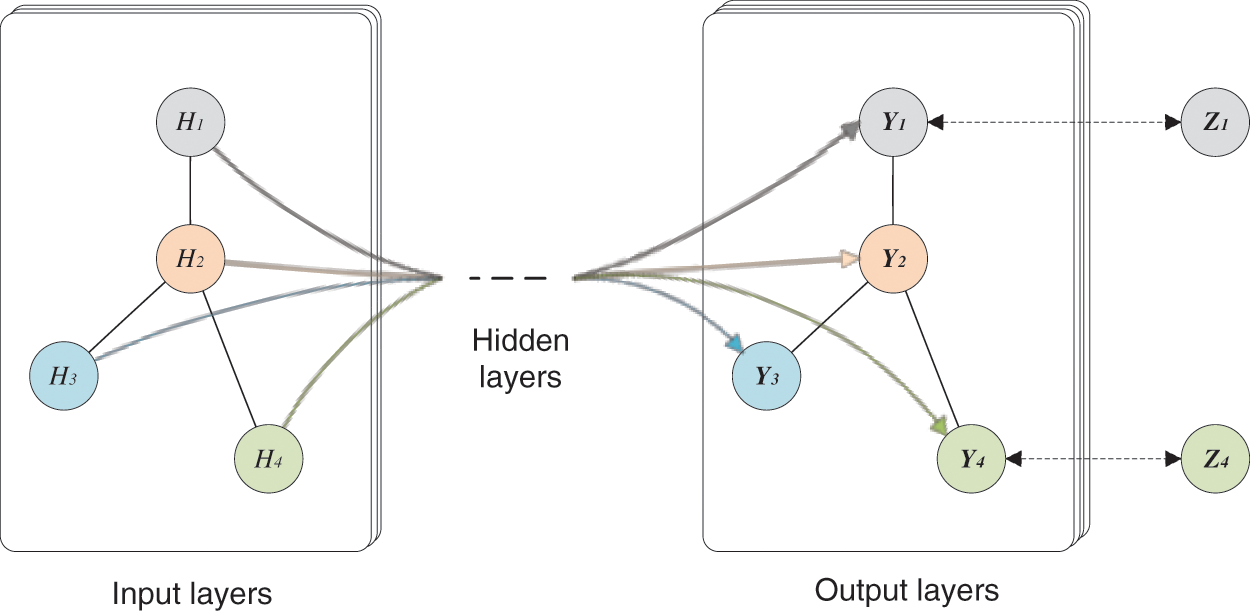
Figure 2: General structure of the GCN

The GCN is also a neural network layer, and the features of each layer need to be calculated with the adjacency matrix A, which represents the relationship between two nodes. The propagation between two layers is expressed as follows:

Y=g(H,A),(1)

H(ι+1)=σ(D~−12 A ~D~−12 H(ι) W(ι)),(2)

where A~=A+I, I is the identity matrix, D~ is the degree matrix of A~, σ is the nonlinear activation function, W is the parameter matrix, D~−12A~D~−12 is the Laplacian matrix for the input layer H(0)=X(0); H(ι) is the feature of l of the GCN.

The training of the GCN module proposes boundary-specific loss functions to optimize learning by combining the cross-entropy loss function, self-guided cross-entropy loss function [48] and Boundary Loss [49] function. Csurka et al. [50] proposed a novel boundary metric, BF1, that accounts for the accuracy of contour extraction and overcomes the weaknesses of mainstream performance measures. The Boundary Loss used in our study is a differentiable surrogate of BF1, resolving the problem that widely-used segmentation loss functions such as binary cross entropy (BCE) loss, IoU loss or Dice loss do not penalize misalignment of boundaries sufficiently. We combine the cross-entropy loss function, self-guided cross-entropy loss function and Boundary Loss function and assign different weight parameters to each loss function for different boundary characteristics to improve the problem of inaccurate boundary classification. The Boundary Loss function is expressed as follows:

L(f^, f)=1−2PQP+Q,(3)

P=1|f|^∑x∈f^⁡{d(x,f)<θ},(4)

Q=1|f|∑x∈f⁡{d(x,f^)<θ},(5)

where {⋅} denotes the logical function, d(⋅) denotes the Euclidean distance between two pixels, and θ denotes the threshold value of Euclidean distance, here distance is calculated from a point to one of two sets (ground truth or predicted boundary) as the shortest distance from the point to the point of the boundary. f^ denotes the semantic segmentation result of the boundary part, and f denotes the label of the boundary part.

2.3 Feature Fusion Classification Module

For the semantic segmentation of remote sensing images, the goal is to determine the accurate localization of all contents in the image and the classification of the target object. Due to different model structures and feature extraction methods, shallow low-level features and in-deep semantic features become the main factors affecting the accuracy of image segmentation [51]. The semi-supervised classification model greatly improves the classification accuracy by integrating the relational information and feature information of image data [52]. Inspired by this idea, the relationship features between objects extracted by the GCN module are used to fuse the features obtained by the image semantic feature extraction module to obtain the final prediction results through the upsampling process. The specific approach is first to expand the feature map extracted from image features into a one-dimensional vector of m×n×Fl, where Fl denotes the number of features extracted by convolution at the l layer. Then, this one-dimensional vector is fed into the GCN model, and the relationship between the features is learned through the graph convolution operation. The features learned by the GCN model in the first layer of convolution can be expressed as follows:

H(1)=σ(D~−12 A ~D~−12 H(ι) W(0)),(6)

where W0 and D~ are the same as those represented by Eq. (2). Second, to ensure the consistency in dimensionality between the feature extraction model and the GCN model in learning the obtained image features, the fully connected layer is added to the GCN module in this paper, and the process is represented as follows:

H(L)=ReLU(Wfc(ReLU(D~−12 A ~D~−12 H(L−1) W(L−1)))),(7)

Last, the feature values and relational information obtained from the image feature extraction module and graph convolutional neural network module are combined, which can be expressed as follows:

y^=softmax(H(L)+V(L′)),(8)

where H(L) is the relational feature extracted by the GCN module, V(L′) is the sample feature, and L′ is the number of layers of ResNet101 and DeepLab V3+ networks in the feature extraction module.

The DGCN model proposed in this paper consists of three steps: image feature extraction module, graph convolutional neural network module and feature fusion, which is briefly described in Algorithm 1.

3  Experiment

3.1 Experimental Data

In this section, experiments are conducted on two publicly available remote sensing image datasets: DeepGlobe [53] and ISPRS 2D [54].

The DeepGlobe land cover classification dataset provides 1146 satellite images of 2448 × 2448 pixels in size; they are RGB images with a pixel resolution of 0.5 m. The dataset features diverse land cover types and high annotation density and is labeled with seven classifications, urban, agriculture, rangeland, forest, water, barren, and unknown, as shown in Table 1. The dataset was divided into a training set, validation set, and test set, containing 803 images, 171 images, and 172 images, respectively, which were cropped to a size of 256 pixels × 256 pixels and reused as the training set, validation set, and test set, with proportions of 75%, 15%, and 15%.

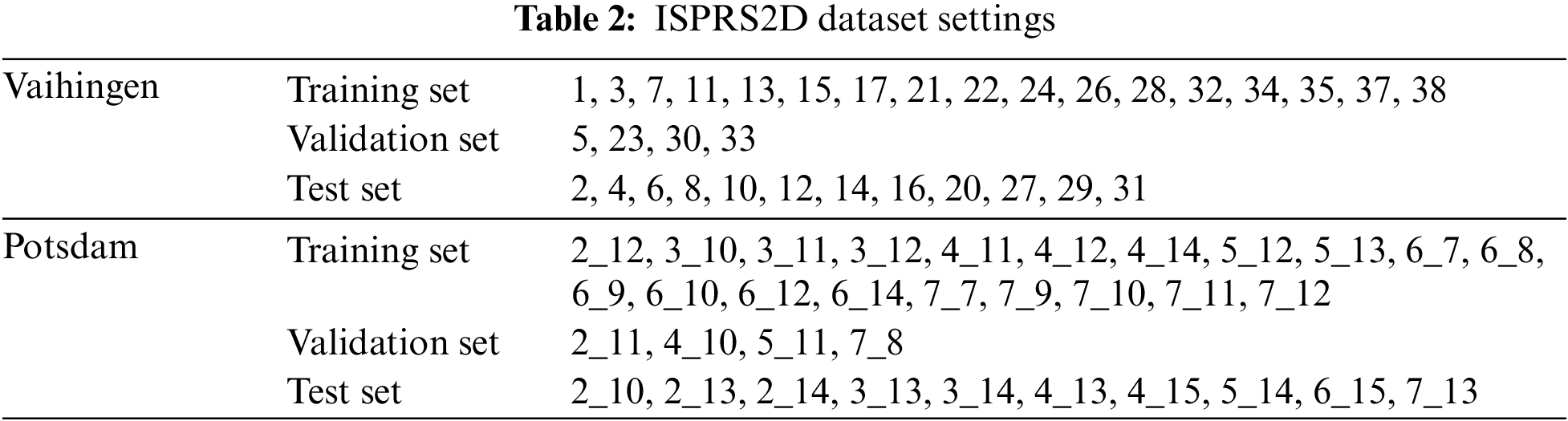
The ISPRS2D semantic segmentation dataset includes the aerial image data of the Vaihingen and Potsdam areas. The Vaihingen area contains 33 remote sensing images with semantic labels. The spatial resolution is 0.09 m, the image size is (1000∼4000) pixels × (1000∼4000) pixels, and the remote sensing images contain near-infrared (NIR), red (R) and green (G) bands. The Potsdam area contains 38 remote sensing images with semantic labels, the spatial resolution is 0.05 m, the image size is 6000 pixels × 6000 pixels, the remote sensing images contain red (R), green (G), and blue (B) bands. The six classifications, including ground, buildings, trees, cars, low vegetation, and unknown. The data settings are shown in Table 2. Since the single image size of the high-resolution image data in the ISPRS2D semantic segmentation dataset is too large, the images in the dataset are cropped to images with a size of 256 pixels × 256 pixels. Mirror flip and rotate to increase the number of training samples, and 20,000 images were trained.

3.2 Evaluation Indicators

In this study, the overall accuracy (OA), mean intersection ratio (mIoU), and F1-score were selected as evaluation metrics and calculated as follows:

OA=TP+TNTP+TN+FP+FN,(9)

F1−score=2×TP2×TP+FP×FN,(10)

mIoU=1m∑i=0mTPFN+FP+TP,(11)

where m denotes the number of categories, TP denotes the number of pixels correctly categorized, FP denotes the number of pixels where the background is determined as the target, FN denotes the number of pixels for which the target is determined as the background, TN denotes the number of pixels for which the target is determined as the background.

3.3 Experimental Setup

In this paper, two corresponding DGCNs, DGCN1 and DGCN2, are designed based on the ResNet101 and DeepLab V3+ networks. In the part of depth feature extraction, stochastic gradient descent (SGD) and cross-entropy serve as the optimizer and loss function, respectively. We set the learning rate to e−5, the weight decay to 0.0005, the number of training iterations to 50, and the batch size to 8. The extracted depth features are used to initialize the graph nodes. In the training of the GCN module, Adam is selected as the optimizer for gradient descent, and the loss functions are the cross-entropy loss function, self-guided cross-entropy loss function and boundary loss function. We set parameter θ to 10, the learning rate to e−5 in the convolutional layer, the weight decay to 0.0005, the number of training iterations to 40, and the batch size to 8.

Our experiments implement our proposed model on a Windows 64-bit system based on an NVIDIA 1080Ti GPU under the TensorFlow framework.

3.4 Comparison Experiments

To verify the effectiveness of the proposed method, the DGCN1 and DGCN2 models proposed in this paper are qualitatively and quantitatively compared with ResNet101, SegNet, U-Net, fully convolutional networks (FCN), DeepLab V3+, DDSSN [41], AttResUNet [33], and FCN using the FCN-8 s model proposed by Long et al. [55]. The semantic segmentation results of different models on ISPRS 2D and DeepGlobe datasets are visually presented and qualitatively analyzed.

The visualization results of the orthophotos of the ISPRS2D test set and their corresponding labels with different models are shown in Fig. 3. The visualization results show the overall segmentation effect of the DGCN1 and DGCN2 models proposed in this paper is better than that of the previous semantic segmentation models. SegNet, U-Net and ResNet101 misclassify some low vegetation as trees; ResNet101 easily misclassifies the unknown type as the ground; DGCN1 better segments low vegetation and trees; FCN is prone to misclassify the unknown type as cars; DeepLab V3+ and DGCN2 better classify cars; the segmentation accuracy of DDSSN is improved at the boundary of the building, but the recognition effect of the spot inside the ground object is poor; and DGCN1 and DGCN2 classify the junction of building land and low vegetation significantly better than other models. All eight semantic segmentation models have the phenomenon of misclassification with low vegetation and the ground. Still, the DGCN1 and DGCN2 models achieve better results overall, with a smaller proportion of misclassified pixels.

Figure 3: Semantic segmentation results of different models on the ISPRS2D test set. (A) and (B) are raw images and tags, respectively. (C) are the results of SegNet. (D) are the results of U-Net. (E) are the results of FCN. (F) are the results of ResNet101, respectively. (G) are the results of DeepLab V3+. (H) are the results of DDSSN. (I) and (J) are the results of DGCN1 and the results of DGCN2, respectively

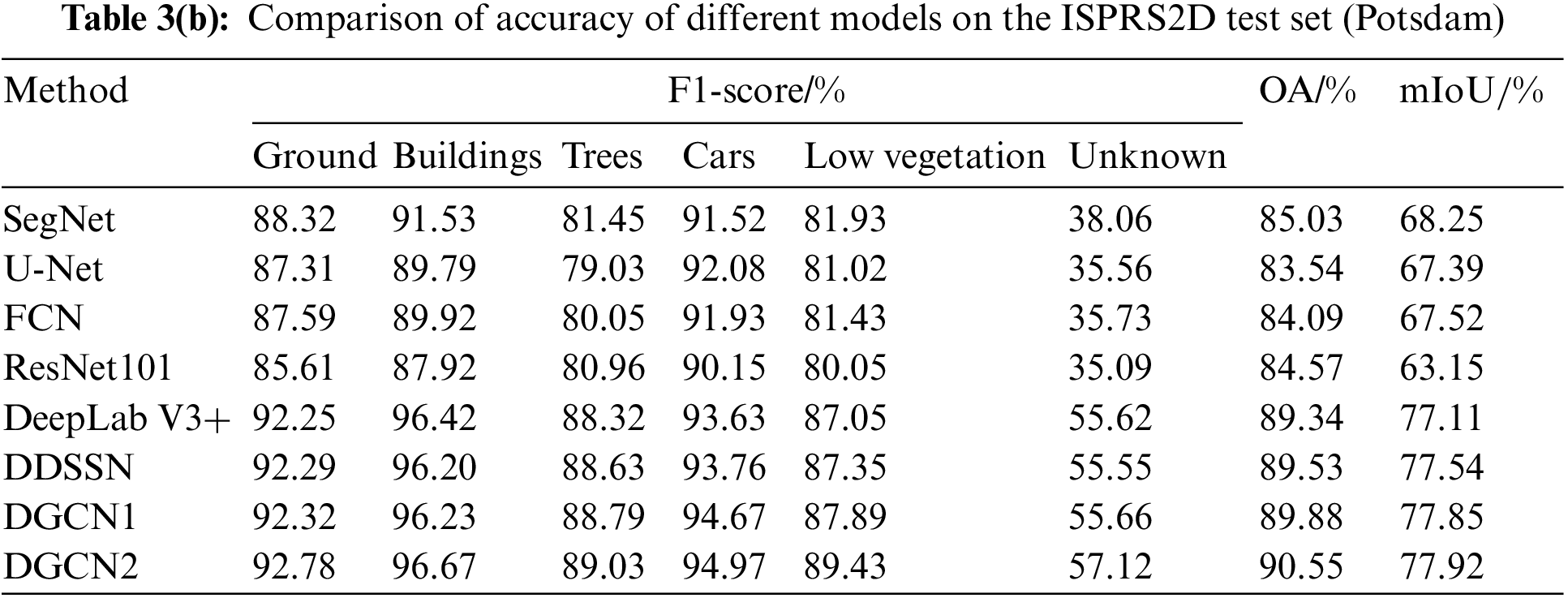
The semantic segmentation accuracies of the models proposed in this paper and other comparison on the test sets in the Vaihingen and Potsdam regions are shown in Tables 3a and 3b. On the dataset in the Vaihingen region, the OA and mIoU of the DGCN1 and DGCN2 models proposed in this paper are the highest; the OA and mIoU for DGCN1 are 2.56% and 5.66% higher, respectively, than ResNet101; and the OA and mIoU for DGCN2 is 0.95% and 4.11% higher, respectively, than DeepLab V3+. Regarding F1-score accuracy metrics, the DGCN2 model achieves 54.39% accuracy for unknown types, which is at least 10% higher than other models, and the DGCN1 and DGCN2 models achieve an accuracy above 94% for building types, which is 1%–3% higher than other models. On the Potsdam area dataset, the OA and mIoU of DGCN1 improved by 5.31% and 5.66%, respectively, compared with ResNet101, and the OA and mIoU of DGCN2 improved by 5.31% and 5.66%, respectively, compared with DeepLab V3+. In terms of the F1-score accuracy metrics, the accuracy of the DGCN1 model for the trees and car types improved by 7.83% and 4.52%, respectively, over ResNet101, and the accuracy of the DGCN2 model for ground and low vegetation types improved by 0.53% and 1.18%, respectively, over DeepLab V3+. Overall, the accuracy of the DGCN1 and DGCN2 models outperformed the other models, which proved the effectiveness of the models in this paper.

The orthoimages of the DeepGlobe test set and their corresponding labels and the visualization result graphs of different models are shown in Fig. 4. SegNet does not classify the agriculture and rangeland boundary parts well, and might completely ignore urban when urban is included in agriculture, ignore rangeland when rangeland is next to the large area of water. U-Net easily misclassify rangeland as forest, U-Net models misclassify forest as agriculture, and U-Net and FCN models misclassify rangeland as water. ResNet101 and AttResUNet easily misclassify agriculture as rangeland. DeepLab V3+ improved the classification of the boundary areas between urban and rangeland, but rangeland was misclassified as barren in some areas. Compared with other semantic segmentation models, the DGCN1 and DGCN2 models proposed in this paper have apparent advantages in classifying the junction of agricultural, urban and rangeland with more explicit feature boundaries and effective noise reduction.

Figure 4: Semantic segmentation results of different models on the DeepGlobe test set. (A) and (B) are raw images and tags, respectively. (C) are the results of SegNet. (D) are the results of U-Net. (E) are the results of FCN. (F) are the results of ResNet101, respectively. (G) are the results of DeepLab V3+. (H) are the results of AttResUNet. (I) and (J) are the results of DGCN1 and the results of DGCN2, respectively

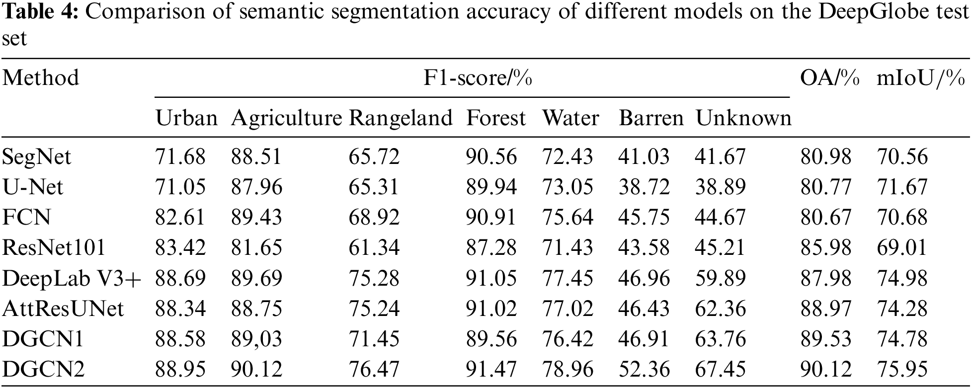
The semantic segmentation accuracies of the model proposed in this paper and other comparison on the DeepGlobe test set are shown in Table 4. The OA and mIoU of DGCN1 improved by 3.55% and 5.77%, respectively, compared with ResNet101, and the OA and mIoU of DGCN2 improved by 2.14% and 0.97%, respectively, compared with DeepLab V3+. In terms of the F1-score accuracy metrics, the accuracy of the DGCN1 model for the rangeland and unknown types improved by more than 10% over ResNet101, and the accuracy of the DGCN2 model for the water and barren types improved by 1.51% and 5.4%, respectively, over DeepLab V3+. Overall, the OA and mIoU of the DGCN1 model and DGCN2 model, respectively, are significantly improved compared with those of the other models, which proves the effectiveness of the models in this paper.

The results of visualization semantic segmentation on DeepGlobe and ISPRS2D data sets show that the segmentation results of DGCN1 and DGCN2 are more comprehensive, with less noise and higher accuracy, indicating that the DGCN can effectively enhance the semantic segmentation effect. Since the GCN module with optimized spatial relations can effectively retain the surface object boundary information while reducing the noise, the segmentation results of DGCN are closer to the actual surface object boundary. The model proposed in this paper makes the internal information of ground feature elements more complete through the hierarchical fusion process of the extracted feature information of each layer, thus confirming the effectiveness of the DGCN model.

3.5 Ablation Study

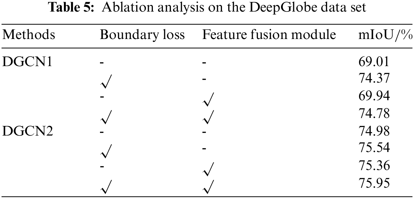
To further illustrate the effectiveness of the proposed method, we performed relevant ablation experiments on the DeepGlobe dataset. The experimental results are shown in Table 5. The baseline models of DGCN1 and DGCN2 obtain mIoU of 69.01% and 74.98%, respectively. By stacking different strategies, consistent improvement over the baseline is achieved. Concretely speaking, Boundary Loss brings mIoU improvement of 5.36% and 0.56%, respectively; the feature fusion module brings mIoU improvement of 0.93% and 0.38%, respectively; our full models have improvement of 5.77% and 0.95%, respectively. These results demonstrate the effectiveness of our model.

4  Conclusion

To address the problems of missing feature boundary information due to convolution and downsampling operations and increasing noise within features due to feature fusion when the existing combined CNN and GCN models are utilized for semantic segmentation, we proposed the DGCN model for semantic segmentation of remote sensing images. The DeepLab V3+ network, which is optimized for boundary information, and the ResNet101 network, which contains more spatial information in the feature map, are selected as the base network to extract deep features of remote sensing images. The GCN module is used to extract spatial relationship information between two features, and the boundary information of features is optimized by using a boundary-specific loss function in the training phase of the GCN module. In the feature fusion stage, a hierarchical feature fusion method is introduced to refine the extracted deep features and spatial relationship information before hierarchical fusion, which effectively solves the problems of internal noise of features and inaccurate boundaries between two target features in the segmentation results. Since inter-object boundary information is crucial to the semantic segmentation of remote sensing images with high accuracy and decipherability, the classification accuracy of remote sensing images is effectively enhanced by fully extracting and utilizing the spatial relationship information of features in the GCN. Experiments were conducted on the ISPRS2D and DeepGlobe datasets. Compared with the ResNet101, SegNet, U-Net, FCN, DeepLab V3+, DDSSN and AttResUNet models, the three accuracy evaluation indices F1-score, OA, and mIoU of the DGCN1 and DGCN2 models proposed in this paper are higher than those of the other models, which confirms the effectiveness of the models in semantic segmentation of remote sensing image. This paper fully optimizes and utilizes the spatial relationship between two target features and dramatically improves the classification effect at the feature boundaries but disregards the degree of influence between two different features. In future research, we will optimize the network structure and introduce the attention mechanism to improve further the optimization ability of spatial relationship information on segmentation accuracy.

Acknowledgement: This research is supported by the Major Scientific and Technological Innovation Project of Shandong Province, Grant No. 2022CXGC010609.

Funding Statement: This research was funded by the Major Scientific and Technological Innovation Project of Shandong Province, Grant No. 2022CXGC010609.

Conflicts of Interest: The authors declare they have no conflicts of interest to report regarding the present study.

References

1. L. Yuan, Q. He, S. Y. Tan, B. Li, J. S. Yu et al., “CoopEdge: A decentralized blockchain–based platform for cooperative edge computing,” in Proc. the Web Conf. (WWW2021), Ljubljana, Slovenia, pp. 2245–2257, 2021. [Google Scholar]

2. F. Wang, G. S. Li, Y. L. Wang, W. Rafique, M. R. Khosravi et al., “Privacy–aware traffic flow prediction based on multi–party sensor data with zero trust in smart city,” ACM Transactions on Internet Technology, 2022. https://doi.org/10.1145/3511904 [Google Scholar] [CrossRef]

3. Y. Zhang, J. Pan, L. Y. Qi and Q. He, “Privacy–Preserving quality prediction for edge-based IoT services,” Future Generation Computer Systems, vol. 114, no. 2021, pp. 336–348, 2021. [Google Scholar]

4. Q. R. Wang, C. C. Zhu, Y. W. Zhang, H. Zhong, J. Q. Zhong et al., “Short text topic learning using heterogeneous information network,” IEEE Transactions on Knowledge and Data Engineering, 2022. https://doi.org/10.1109/TKDE.2022.3147766 [Google Scholar] [CrossRef]

5. W. W. Gong, C. Lv, Y. C. Duan, Z. G. Liu, M. R. Khosravi et al., “Keywords-driven web APIs group recommendation for automatic app service creation process,” Software: Practice and Experience, vol. 51, no. 11, pp. 2337–2354, 2020. [Google Scholar]

6. Y. Li, J. Liu, B. Cao and C. G. Wang, “Joint optimization of radio and virtual machine resources with uncertain user demands in mobile cloud computing,” IEEE Transactions on Multimedia, vol. 20, no. 9, pp. 2427–2438, 2018. [Google Scholar]

7. L. Y. Qi, Y. H. Yang, X. K. Zhou, W. Rafique and J. H. Ma. “Fast anomaly identification based on multi-aspect data streams for intelligent intrusion detection toward secure industry 4.0,” IEEE Transactions on Industrial Informatics, vol. 18, no. 9, pp. 6503–6511, 2022. [Google Scholar]

8. Y. Li, C. Liao, C. G. Wang and Y. Wang. “Energy-efficient optimal relay selection in cooperative cellular networks based on double auction,” IEEE Transactions on Wireless Communications, vol. 14, no. 8, pp. 4093–4104, 2015. [Google Scholar]

9. Y. Li, S. C. Xia, M. Y. Zheng, B. Cao and Q. L. Liu, “Lyapunov optimization based trade-off policy for mobile cloud offloading in heterogeneous wireless networks,” IEEE Transactions on Cloud Computing, vol. 10, no. 1, pp. 491–505, 2022. [Google Scholar]

10. L. Y. Qi, W. M. Lin, X. Y. Zhang, W. C. Dou, X. L. Xu et al., “A correlation graph based approach for personalized and compatible Web APIs recommendation in mobile APP development,” IEEE Transactions on Knowledge and Data Engineering, 2022. https://doi.org/10.1109/TKDE.2022.3168611 [Google Scholar] [CrossRef]

11. Q. Liu, N. Y. Zhang, W. Z. Yang, S. Wang, Z. C. Cui et al., “A review of image recognition with deep convolutional neural network,” in Proc. Intelligent Computing Theories and Application: 13th Int. Conf., Liverpool, UK, pp. 69–80, 2017. [Google Scholar]

12. F. Sultana, A. Sufian and P. Dutta, “A review of object detection models based on convolutional neural network,” in Intelligent Computing: Image Processing Based Applications, Singapore: Springer Press, pp. 1–16, 2020. [Google Scholar]

13. J. Y. Chai and A. M. Li, “Deep learning in natural language processing: A state-of-the-art survey,” in Proc. 2019 Int. Conf. on Machine Learning and Cybernetics (ICMLC), Kobe, Japan, pp. 1–6, 2019. [Google Scholar]

14. E. Basaeed, H. Bhaskar and M. Al-Mualla, “Supervised remote sensing image segmentation using boosted convolutional neural networks,” Knowledge–Based Systems, vol. 100, no. 99, pp. 19–27, 2016. [Google Scholar]

15. D. Feng, C. Haase-Schütz, L. Rosenbaum, H. Hertlen, C. Gläser et al., “Deep multi-modal object detection and semantic segmentation for autonomous driving: Datasets, methods, and challenges,” IEEE Transactions on Intelligent Transportation Systems, vol. 22, no. 3, pp. 1341–1360, 2020. [Google Scholar]

16. H. Lee and H. Kwon, “Going deeper with contextual CNN for hyperspectral image classification,” IEEE Trans. on Image Process, vol. 26, no. 10, pp. 4843–4855, 2017. [Google Scholar]

17. R. Irfan, A. A. Almazroi, H. T. Rauf, R. Damaševičius, E. A. Nasr et al., “Dilated semantic segmentation for breast ultrasonic lesion detection using parallel feature fusion,” Diagnostics, vol. 11, no. 7, pp. 1212, 2021. [Google Scholar] [PubMed]

18. Z. F. Zhang, X. Cui, Q. Zheng and J. Cao. “Land use classification of remote sensing images based on convolution neural network,” Arabian Journal of Geosciences, vol. 14, no. 4, pp. 1–6, 2021. [Google Scholar]

19. E. D. Wang, K. Qi, X. P. Li and L. Y. Peng, “Semantic segmentation of remote sensing image based on neural network,” Acta Optica Sinica, vol. 39, no. 12, pp. 93–104, 2019. [Google Scholar]

20. S. P. Ji, S. Q. Tian and C. Zhang, “Urban land cover classification and change detection using fully atrous convolutional neural network,” Geomatics and Information Science of Wuhan University, vol. 45, no. 2, pp. 233–241, 2020. [Google Scholar]

21. Z. F. Shao, Y. M. Sun, J. B. Xi and Y. Li, “Intelligent optimization learning for semantic segmentation of high spatial resolution remote sensing images.” Geomatics and Information Science of Wuhan University, vol. 47, no. 2, pp. 234–241, 2022. [Google Scholar]

22. J. Kang, F. B. Ruben, D. F. Hong, C. Jocelyn and A. Plaza, “Graph relation network: Modeling relations between scenes for multilabel remote-sensing image classification and retrieval,” IEEE Transactions on Geoscience and Remote Sensing, vol. 59, no. 5, pp. 4355–4369, 2021. [Google Scholar]

23. Y. B. Wang, L. Q. Zhang, X. H. Tong, F. P. Nie, H. Y. Huang et al., “LRAGE: Learning latent relationships with adaptive graph embedding for aerial scene classification,” IEEE Transactions on Geoscience and Remote Sensing, vol. 56, no. 2, pp. 621–634, 2018. [Google Scholar]

24. L. Z. Kong, G. S. Li, W. Rafique, S. G. Shen, Q. He et al., “Time-aware missing healthcare data prediction based on ARIMA model,” IEEE/ACM Transactions on Computational Biology and Bioinformatics, vol. 2022, no. 1, pp. 1–10, 2022. [Google Scholar]

25. Y. W. Zhang, C. H. Yin and Q. L. Wu, “Location-aware deep collaborative filtering for service recommendation,” IEEE Transactions on Systems, Man, and Cybernetics: Systems, vol. 51, no. 6, pp. 3796–3807, 2021. [Google Scholar]

26. Y. W. Zhang, G. M. Cui, S. G. Deng, F. F. Chen, Y. Wang et al., “Efficient query of quality correlation for service composition,” IEEE Transactions on Services Computing, vol. 14, no. 3, pp. 695–709, 2021. [Google Scholar]

27. Y. W. Zhang, K. B. Wang and Q. He, “Covering-based Web service quality prediction via neighborhood-aware matrix factorization,” IEEE Transactions on Services Computing, vol. 14, no. 5, pp. 1333–1344, 2021. [Google Scholar]

28. K. M. Ding, C. Q. Zhu and F. Q. Lu, “An adaptive grid partition based perceptual hash algorithm for remote sensing image,” Geomatics and Information Science of Wuhan University, vol. 40, no. 6, pp. 716–720+743, 2015. [Google Scholar]

29. L. Z. Kong, L. N. Wang, W. W. Gong, C. Yan, Y. C. Duan et al., “LSH–aware multitype health data prediction with privacy preservation in edge environment,” World Wide Web Journal, vol. 25, no. 5, pp. 1793–1808, 2022. [Google Scholar]

30. W. W. Gong, W. Zhang, M. Bilal, Y. F. Chen, X. L. Xu et al., “Efficient Web APIs recommendation with privacy-preservation for mobile App development in industry 4.0,” IEEE Transactions on Industrial Informatics, vol. 18, no. 9, pp. 6379–6387, 2021. [Google Scholar]

31. S. Ouyang and Y. S. Li, “Combining deep semantic segmentation network and graph convolutional neural network for semantic segmentation of remote sensing imagery,” Remote Sens, vol. 13, no. 1, pp. 119, 2021. [Google Scholar]

32. R. T. Feng, H. F. Shen, J. J. Bai and X. H. Li, “Advances and opportunities in remote sensing image geometric registration: A systematic review of state-of-the-art approaches and future research directions,” IEEE Geoscience and Remote Sensing, vol. 9, no. 4, pp. 120–142, 2021. [Google Scholar]

33. T. N. Kipf, M. Welling, “Semi-supervised classification with graph convolutional networks,” in Proc. 2017 Int. Conf. on Learning Representations, Toulon, French, pp. 1–14, 2017. [Google Scholar]

34. Z. H. Wu, S. R. Pan, F. W. Chen, G. D. Long, C. Q. Zhang et al., “A comprehensive survey on graph neural networks,” IEEE Transactions on Neural Networks and Learning Systems, vol. 32, no. 1, pp. 4–24, 2021. [Google Scholar] [PubMed]

35. D. F. Hong, L. R. Gao, J. Yao, B. Zhang, A. Plaza et al., “Graph convolutional networks for hyperspectral image classification,” IEEE Transactions on Geoscience and Remote Sensing, vol. 59, no. 7, pp. 5966–5978, 2020. [Google Scholar]

36. W. W. Gong, X. Y. Zhang, Y. F. Chen, Q. He, A. Beheshti et al., “DAWAR: Diversity-aware web APIs recommendation for mashup creation based on correlation graph,” in Proc. 45th Int. ACM SIGIR Conf. on Research and Development in Information Retrieval, Madrid, Spain, pp. 395–404, 2022.

37. Y. W. Liu, Z. L. Song, X. L. Xu, W. Rafique, X. Y. Zhang et al., “Bidirectional GRU networks–based next POI category prediction for healthcare,” International Journal of Intelligent Systems, vol. 37, no. 7, pp. 4020–4040, 2022. [Google Scholar]

38. J. L. Liang, Y. F. Deng and D. Zeng, “A deep neural network combined CNN and GCN for remote sensing scene classification,” IEEE Selected Topics in Applied Earth Observations and Remote Sensing, vol. 13, pp. 4325–4338, 2020. [Google Scholar]

39. X. D. Liang, X. H. Shen, J. S. Feng and L. Liang, “Semantic object parsing with graph LSTM,” in Proc. 2016 European Conf. on Computer Vision, Amsterdam, Netherlands, pp. 125–143, 2016. [Google Scholar]

40. Q. C. Liu, L. Xiao, J. X. Yang and Z. H. Wei, “CNN-Enhanced graph convolutional network with pixel-and superpixel-level feature fusion for hyperspectral image classification,” IEEE Transactions on Geoscience and Remote Sensing, vol. 59, no. 10, pp. 8657–8671, 2021. [Google Scholar]

41. S. Liu, X. Y. Li, M. Yu and G. L. Xing, “Dual decoupling semantic segmentation model for high-resolution remote sensing images,” Acta Geodaetica et Cartographica Sinica, 2022. http://kns.cnki.net/kcms/detail/11.2089.P.20220729.0856.002.html [Google Scholar]

42. Q. C. Geng, Z. Zhou and X. C. Cao, “Survey of recent progress in semantic image segmentation with CNNs,” Science China Information Sciences, vol. 61, no. 5, pp. 1–18, 2018. [Google Scholar]

43. L. C. Chen, Y. K. Zhu, G. Papandreou, F. Schroff and H. Adam, “Encoder-decoder with atrous separable convolution for semantic image segmentation,” in Proc. 2018 European Conf. on Computer Vision, Federal, Munich, pp. 801–818, 2018. [Google Scholar]

44. K. M. He, X. Y. Zhang, S. Q. Ren and J. Sun, “Deep residual learning for image recognition,” in Proc. 2016 IEEE Conf. on Computer Vision and Pattern Recognition, Las Vegas, NV, USA, pp. 1063–6919, 2016. [Google Scholar]

45. C. Q. Yu, J. B. Wang, C. Peng, C. X. Gao, G. Yu et al., “Learning a discriminative feature network for semantic segmentation,” in Proc. 2018 IEEE Conf. on Computer Vision and Pattern Recognition, UT, USA, pp. 1857–1866, 2018. [Google Scholar]

46. P. Bilinski and V. Prisacariu, “Dense decoder shortcut connections for single-pass semantic segmentation,” in Proc. 2018 IEEE Conf. on Computer Vision and Pattern Recognition, UT, USA, pp. 6596–6605, 2018. [Google Scholar]

47. S. Ouyang, “The methodology research on geographic knowledge-guided deep semantic segmentation of remote sensing lmagery,” Ph.D. Dissertation, Wuhan University, China, 2021. [Google Scholar]

48. T. J. Yang, M. D. Collins, Y. K. Zhu, J. J. Hwang and T. Liu, “Deeperlab: Single-shot image parser,” in Proc. IEEE Conf. on Computer Vision and Pattern Recognition, California, USA, pp. 10, 2019. [Google Scholar]

49. A. Bokhovkin, E. Burnaey, “Boundary loss for remote sensing imagery semantic segmentation,” in Proc. 2019 Int. Symp. on Neural Networks, Moscow, Russia, pp. 388–401, 2019. [Google Scholar]

50. G. Csurka, D. Larlus and F. Perronnin, “What is a good evaluation measure for semantic segmentation?,” in Proc. 2013 British Machine Vision Conf., London, U.K., pp. 32.1–32.11, 2013. [Google Scholar]

51. X. Q. Zhao and H. P. Xu, “Lmage semantic segmentation method with hierarchical feature fusion,” Frontiers of Computer Science and Technology, vol. 15, no. 5, pp. 949–957, 2021. [Google Scholar]

52. W. Liu, X. Y. Wang, G. W. Liu, D. Wang and Y. J. Niu, “Semi-supervised image classification method fused with relational features,” CAAI Transactions on Intelligent Systems, vol. 17, no. 5, pp. 886–899, 2022. [Google Scholar]

53. I. Demir, K. Koperski, D. Lindenbaum, G. Pang, J. Huang et al., “DeepGlobe 2018: A challenge to parse the earth through satellite images,” in Proc. IEEE Conf. on Computer Vision and Pattern Recognition Workshops (CVPRW), UT, USA, pp. 172–181, 2018. [Google Scholar]

54. F. Rottensteiner, G. Sohn, J. Jung, M. Gerk, C. Baillard et al., “The ISPRS benchmark on urban object classification and 3D building reconstruction,” ISPRS Annals of the Photogrammetry, Remote Sensing and Spatial Information Sciences I-3 (2012), vol. 1, no. 1, pp. 293–298, 2013. [Google Scholar]

55. J. Long, E. Shelhamer and T. Darrell, “Fully convolutional networks for semantic segmentation,” IEEE Transactions on Pattern Analysis and Machine Intelligence, vol. 39, no. 4, pp. 640–651, 2017. [Google Scholar]