Data Layout and Scheduling Tasks in a Meteorological Cloud Environment

1  Introduction

1.1 Background

Several petabytes of big data (such as records, texts, and pictures) are stored in the cloud [1]. Big data management technology has been widely studied theoretically for processing big data, in terms of aspects such as security [2], replica management, fairness [3], processing methods [4], and workflow management [5]. Apache Hadoop [6], Microsoft HDInsight, GFS (Google File System) MapReduce [7], and BigTable are seminal platforms for big data management and processing.

Big data management provides applications in different areas involving various technologies and practices. Currently, many industries have built cloud and big data platforms, which have substantially changed people’s lives. These include platforms for smart urban transportation [8], predicting completion risk [9], drought monitoring [10], dermatology [11], traffic flow prediction [12], urban sustainability research [13], and health care [11], among other applications.

1.2 Challenges and Motivations

Meteorological clouds and big data platforms have also been investigated from various perspectives [14]. Meteorological cloud and big data platforms mainly provide support for meteorological model tasks [15], such as hard disk, memory, and processing tasks. Different from most cloud environments, meteorological platforms also provide large volumes of basic meteorological data. The data may come from multiple sources, such as satellites and basic stations. The meteorological data may vary in terms of scope, time, accuracy, level, and other factors [16]. These data are very important for meteorological model tasks. For example, if a meteorological model task I (located in cloud A) needs meteorological data set α (located in cloud B), then, meteorological set α needs to be transferred from Cloud B to A for the execution of I. Because of the limitations of the size of the hard disks of cloud A, some data (data set β) for the following task II must be deleted. After the execution of task I, meteorological data set β needs to be copied from others clouds. If we give a good layout and scheduling method, we can reduce the time for transferring files and the execution time. In the example, if we can assign task I to A and save meteorological set α in A, at the same time, we assign task II to B and save meteorological set β in B, we can overcome transferring files between clouds, thus reducing the energy consumption and execution time.

This paper focuses on the meteorological data layout problem. Different meteorological model tasks require different types of meteorological basis data support. Different from previous research, we solve the problem using the relations between meteorological datasets and meteorological model tasks. The relation not only includes the interrelation between datasets and tasks but also includes the relation between datasets and tasks. Based on the relation, we lay out meteorological data sets and allocated tasks. Major contributions of our paper include: (1) mining the relation between meteorological models and data sets, (2) layout meteorological data sets according to the relation, (3) scheduling meteorological tasks according to the relation, and (4) evaluating the performance of our scheduling methods based on the data layout.

The remainder of this paper is organized as follows. Section 2 discusses the related work. Section 3 presents the framework of meteorological clouds and the related models that are used in our paper. Section 4 demonstrates how to mine the relationships between meteorological models and meteorological datasets. These relationships are also discussed in Section 4. We present the data layout method in Section 5 and the simulation and comparison in Section 6. Section 7 presents the conclusions of the paper and discusses new research directions for the future.

2  Related Work

Task scheduling in the cloud environment has been widely studied in the past decades. They always model the application as a DAG (Directed Acyclic Graph), and focus on how to allocate VMs to tasks in a DAG. Shu et al. [17] proposed a strong agile response task scheduling optimization algorithm based on the peak energy consumption of data centers and the time span of task scheduling in green computing. Moustafa et al. focused [18] on the problem of cost-aware VM migration in a federated cloud environment. They targeted to maximize the profit of the cloud provider and minimize the cost. They designed a polynomial-time VM migration heuristics to minimize migration time. Gholipour et al. [19] gave a new cloud resource scheduling procedure based on a multi-criteria decision-making method in green computing, that was based on a joint virtual machine and container migration method. A. Javadpour et al. [20] provided an efficient dynamic resources infrastructure management on Software-Based Networks, which used TDMA (Markov Process and the Time Division Multiple Access) protocol to schedule resources. In the edge-cloud environment, Jayanetti et al. [21] leveraged deep reinforcement learning for designing a workflow scheduling framework. They designed a novel hierarchical action space for promoting a clear distinction between edge and cloud nodes, which efficiently deals with the complex workflow scheduling problem. Those methods always pay attention to energy consumption, cost, profit, and so on. Because the data of those tasks are always different, one data set always is used by one task. In other words, they do not take into account the layout of data sets. In the meteorological cloud environment, data sets may be used by different meteorological models (even used by a meteorological model many times), so the above-mentioned methods can not be used for meteorological tasks.

Data layout is a very important problem in the cloud when the data needs to be repeatedly used. As big data become more widely used in industry, data layout becomes increasingly important. The 5 Vs (volume, variety, value, velocity, and veracity) of big data make the data layout in a big data environment more variable than those in other environments, and the data may originate from multiple sources, with large volumes, different locations, and so on, which must be addressed.

Researchers have proposed various data layout methods in distributed systems. Song et al. [22] proposed a cost-intelligent data access strategy that is based on the application-specific optimization principle for improving the I/O performance of parallel file systems. Zaman et al. [23] focused on the multidisk data layout problem by proposing an affinity graph model for capturing workload characteristics in the presence of access skew and providing an efficient physical data layout. Suh et al. [24] used DimensionSlice to optimize a new main-memory data layout. DimensionSlice was used for intracycle parallelism and early stopping in scanning multidimensional data. Zhou et al. [25] proposed ApproxSSD for performing on-disk layout-aware data sampling on SSD (Solid State Disk) arrays. ApproxSSD decoupled I/O from the computation in task execution to avoid potential I/O contentions and suboptimal workload balances. Booth et al. [26] proposed a hierarchical two-dimensional data layout that aimed to reduce synchronization costs in multicore environments. Bel et al. [27] developed Geomancy to model how data layout influenced performance in a distributed storage system.

Some data layout methods also have been proposed for the cloud environment. Liu et al. [28] proposed an adaptive discrete particle swarm optimization (PSO) algorithm that is based on a genetic algorithm for reducing data transmissions between data centers in a hybrid cloud. Jiang et al. [29] proposed a novel efficient speech data processing layout by considering prior information and the data structure in a cloud environment. Considering the differences between speech data that are related to lowercase read-ahead and basic read-ahead scenarios and purposes, they used an efficient robust data mining model to capture the data structure and features. In recent years, a few reinforcement learning methods also have been used for the data layout in the cloud. To enhance the efficiency of Cyber–Physical–Social-Systems applications in edges [30], the memory space at runtime is optimized through data layout reorganization from the spatial dimension by a deep learning inference.

In meteorological clouds [31], including meteorological big data environments, researchers have also provided methods for the layout of meteorological datasets. He et al. [32] used the Hadoop ecosystem and the Elastic search cluster (ES cluster) to build a meteorological big data platform. To improve the efficiency of meteorological data, Yang et al. [33] used multidimensional block compression technology to store and transmit meteorological data. They also used heterogeneous NoSQL common components to increase the heterogeneity of the NoSQL database. Ruan et al. [34] used a fat-tree topology to analyze resource utilization and other aspects of meteorological cloud platforms. They used the NSGA-III (Nondominated Sorting Genetic Algorithm III) to lay out meteorological data, to optimize resource utilization and other aspects. These methods ignore that meteorological data are always used by meteorological models. Different models need different meteorological data. The data vary in time and space. In this paper, we try to lay out the data based on the relationships between meteorological models and meteorological data.

Different from previous methods, our paper attempts to solve the data layout problem by considering the relations between meteorological models and meteorological datasets. Past works have always ignored that a meteorological model always needs the same basic meteorological datasets (with little change, and the size can be ignored).

3  System Framework and Models

3.1 System Framework

As illustrated in Fig. 1, the State Meteorological Administration (SMA) administers all data and dispatches them to the cloud centers of various provinces. It collects data using satellites, and some datasets may be based on meteorological stations. Clouds 1~3 belong to different places (different provinces). They have access to the data center in SMA. Clouds 1~3 obtain datasets from SMA when they need data for the execution of meteorological model tasks. When the required datasets are not located on the cloud where a task is executed, the task needs time to prefetch those datasets from SMA. Because the data in SMA are dynamic, all datasets in the clouds should remain the same as the datasets in SMA. Although meteorological model tasks require larger volumes of input files, they always produce small volumes of output files (we can even regard the output volumes as zero).

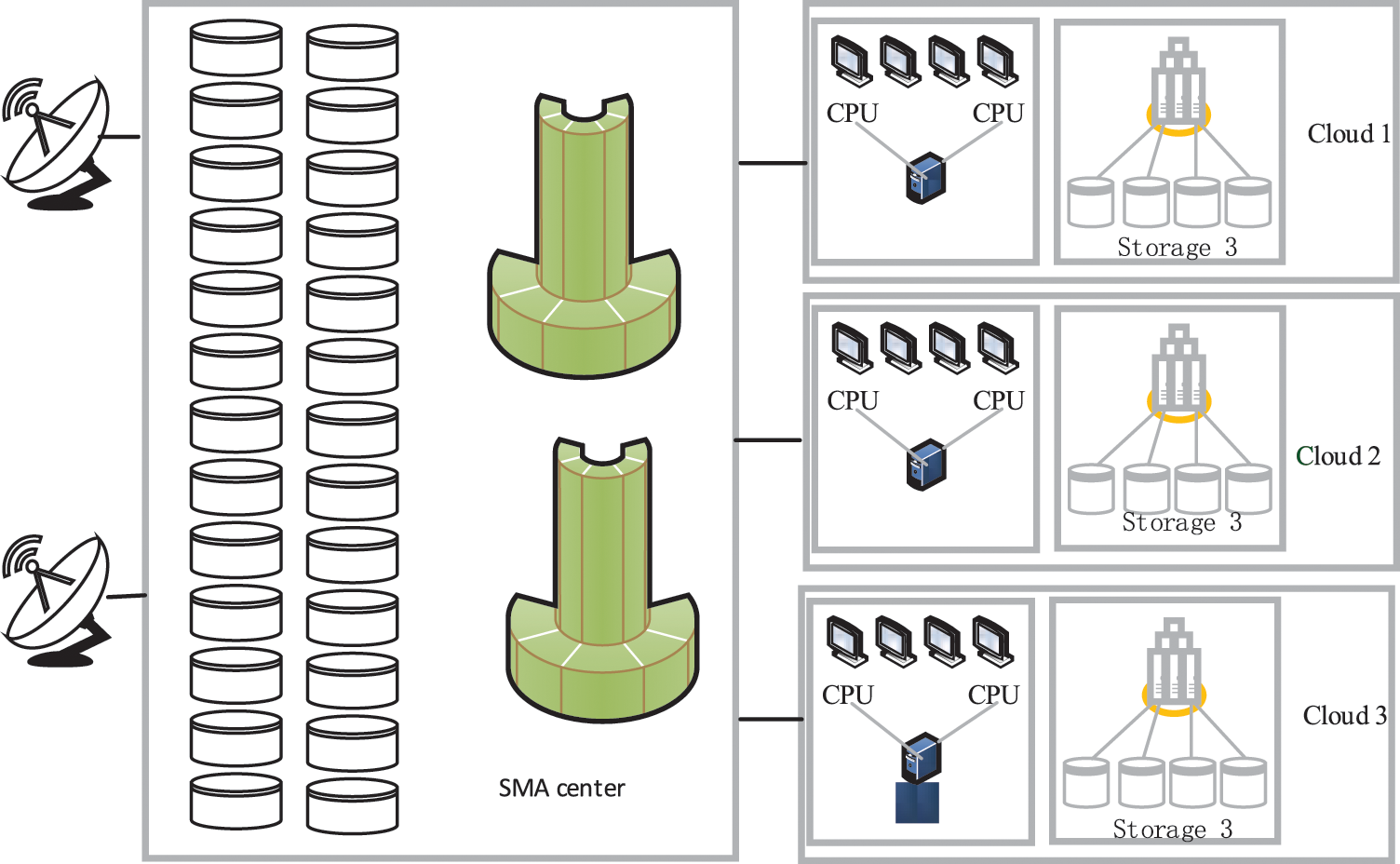
Figure 1: System framework of the state meteorological administration

In this paper, we suppose that SMA has enough capacity for saving all meteorological datasets. In other words, all meteorological datasets have at least one copy on hard SMA disks. Because every cloud is in charge of the data collection, when they get a new data set, it needs to transfer it to the SMA. If a cloud wants to get a new data set, it can get a copy from CMA. Of course, it also can get data from the cloud nearby (with a higher bandwidth between clouds). We can regard the meteorological regional forecasting model for different places as two different meteorological models. For example, the WRF model for Anhui Province and Jiangsu Province may be regarded as two models, namely, WRF-Anhui and WRF-Province, because they need different meteorological datasets. Our framework can save space of hard disks and one meteorological data set only needs one copy in the cloud.

3.2 Models for Meteorological Systems

We suppose that there are Mnum kinds of meteorological models and Dnum datasets for those meteorological models:

M={m1,m2…mmid…,mMnum}(1)

D={d1,d2…ddid…,dDnum}(2)

Meteorological model mmid needs dataset ddid. The size of ddid is dsdid:

DS={ds1,ds2…dsdid…,dsDnum}(3)

Different models may use the same meteorological datasets. For example, meteorological model A may use datasets d1 and d2, and meteorological model B may use datasets d2, d3 and d4. We hope we can lay out the datasets and schedule each meteorological model according to the degree of correlation between the datasets and the meteorological model.

4  Mining the Relationships Based on Meteorological Scheduling Logs

4.1 An Introduction to the Log

A record in the log includes information about the meteorological models that are used and the relative meteorological basis data. As shown in Fig. 2, the scheduling log can be taken as a record with Mnum+Dnum bits. The former Mnum bits record which meteorological models have been used, and the latter Dnum bits record which dataset has been used for scheduling. Table 1 presents a log with 20 scheduling records.

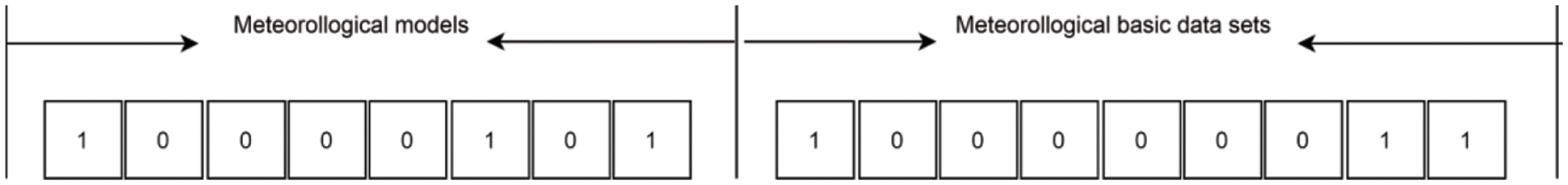
Figure 2: A record in the scheduling log

4.2 Mining the Relationships in the Log

In this section, we use the FP-Growth method to mine the relations (1) between meteorological models, (2) between meteorological datasets, and (3) between meteorological models and datasets.

4.2.1 FP Mining of the Relationships between Meteorological Models (FI1)

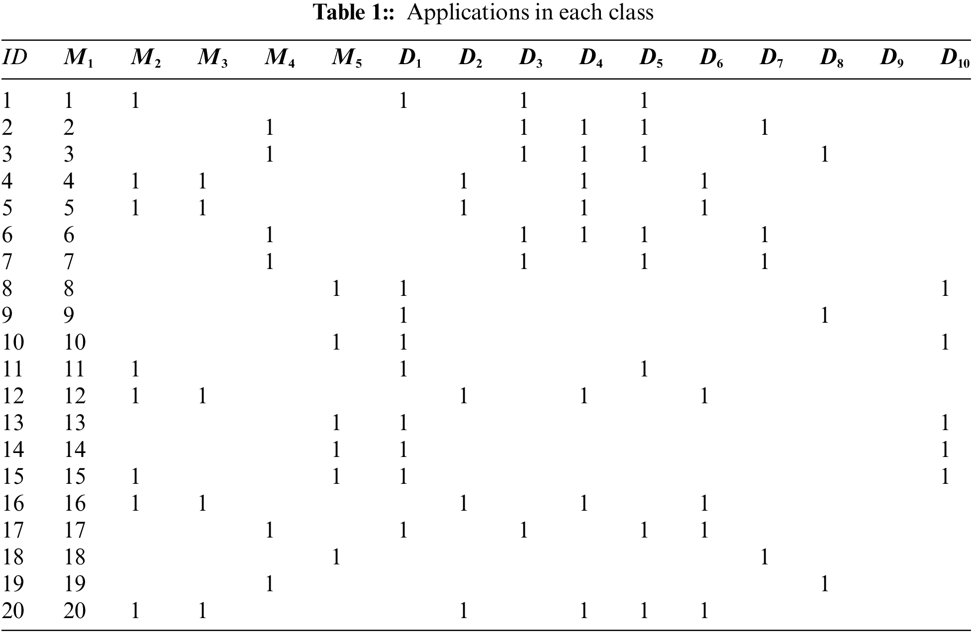
We use the FP-Growth method to mine the frequent itemsets in meteorological models. Here, we only consider Columns 1~5 of Table 1. The steps are presented in detail in Algorithm 1.

We set the minimum support (ms1) to 20%, and the frequent itemsets are:

FI1(ms1)={(m1,m2),(m4,m5),(m3)}(4)

Fig. 3a is the main flow diagram of our methods and Fig. 3b is the main diagram of Algorithm 1 (also denoted the main step of Fig. 3a). First, we scan the log to obtain the count of all frequent 1 -itemsets. We delete items whose support degree is lower than the threshold (minv). The frequent 1-itemsets are inserted into the item header table (T) and arranged in descending order of support degree. We remove the nonfrequent 1-itemsets by scanning data, and they are arranged in descending order of support degree. The sorted dataset (P) is inserted into the FP tree in sorted order. Each node at the top of the sorted tree is an ancestor node, while each node at the bottom is a descendant node. If there is a common ancestor, the corresponding common ancestor node count is increased by 1. After insertion, if a new node appears, the node that corresponds to the item header table is connected to the new node via a node chain. The FP tree is established when all data (p) have been inserted into the FP tree. The conditional pattern sets that correspond to the item header items are identified in turn from the bottom item of the item header table. Frequent itemsets are obtained by recursively mining conditional pattern sets.

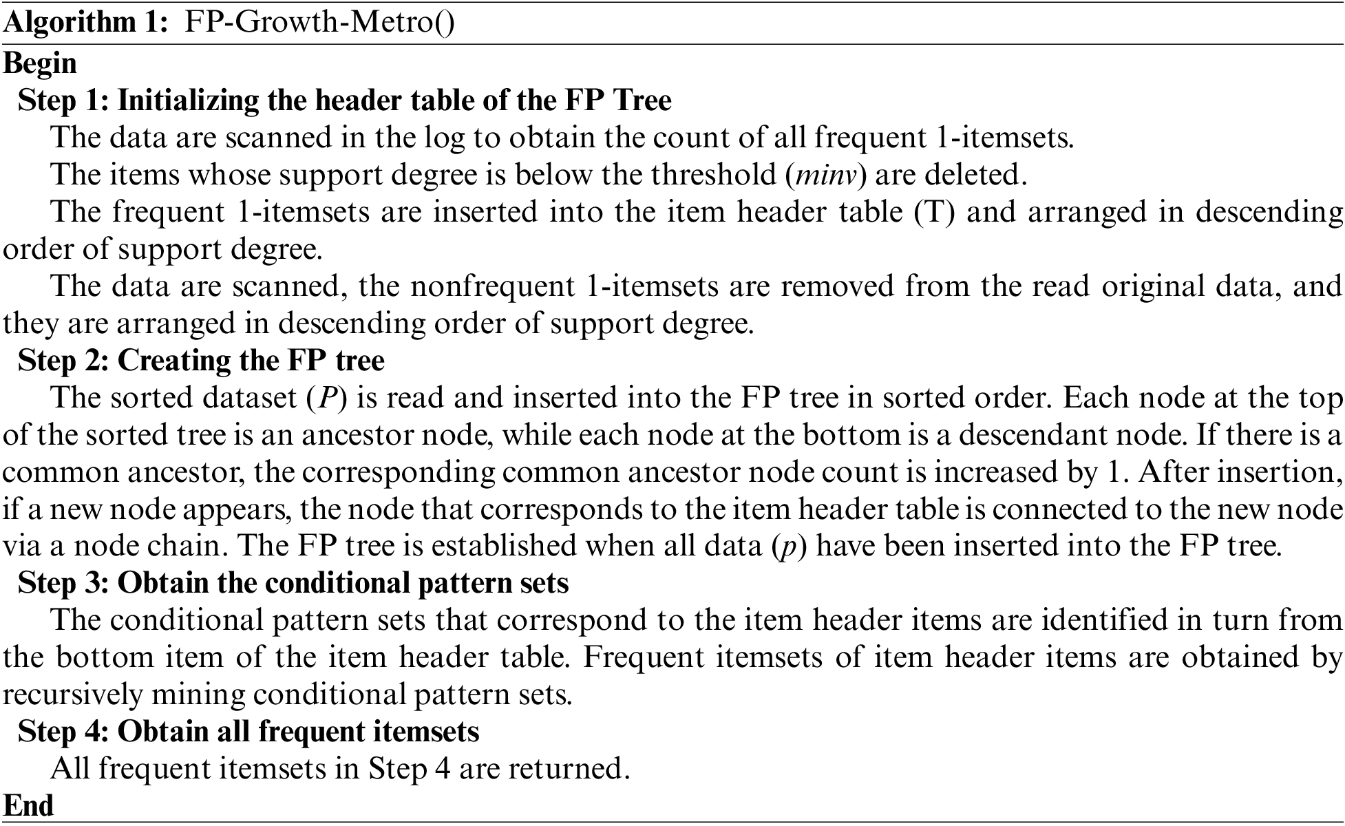
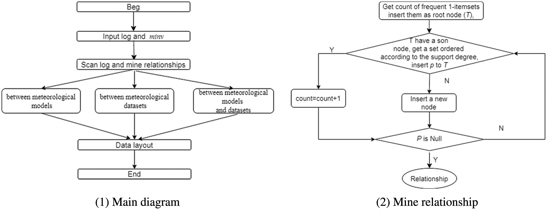
Figure 3: Flow diagram of our method

4.2.2 FP Mines the Relationships between Meteorological Datasets (FI2)

Similar to Algorithm 1, we also use FP-Growth to mine the relationships between meteorological datasets. Because the method is the same as that described by Algorithm 1, we do not present the details here. We set the minimum support degree (ms2) to 20%, and the frequent itemsets are

FI2(ms2)={(d1,d2,d5),(d9,d10),(d2,d4,d6)}(5)

4.2.3 FP Mining of the Relationships between Meteorological Model Tasks and Meteorological Datasets (FI3)

As in the method that was used in Section 4.2.1, FP-Growth can also be used to mine the relationships between meteorological tasks and meteorological datasets. We set the minimum support degree (ms3) to 25%. The frequent itemsets are:

FI3(ms3)={(m1,m2,d1,d3,d5)}(6)

Here, we always select ms3>ms1 and ms3>ms2. The reason is that meteorological models and meteorological datasets are always larger than their interior models and datasets.

4.3 Analysis of the Relationships Based on Data Mining

The itemsets in FI1, FI2 and FI3 have different meanings:

(1)   The frequent itemsets of FI1 correspond to meteorological models that are always scheduled by a task;

(2)   The frequent itemsets of FI2 correspond to meteorological datasets that are always used by a task;

(3)   he frequent itemsets of FI3 correspond to meteorological datasets and meteorological models that are always scheduled by a task.

Based on the analysis above, we can use the information to facilitate the data layout of meteorological datasets and the scheduling of meteorological model tasks:

(1)   We allocate meteorological models in the frequent itemsets of FI1 in the same data center to reduce the number of clouds that a meteorological model utilizes;

(2)   We lay out the meteorological datasets in the frequent itemsets of FI2 in the same data center to reduce the number of copies of the meteorological datasets;

(3)   We allocate the meteorological models and lay out the meteorological datasets in the frequent itemsets of FI3 in the same data center to reduce the sizes of the files that are transferred between data centers.

5  A Heuristic Data Layout Algorithm for Meteorological Datasets

Section 5.1 presents the models that are used in our paper. Section 5.2 describes the data layout method and task scheduling method in meteorological clouds.

5.1 Models Used in Meteorological Clouds

There are Cnum meteorological clouds, where cid is the cloud identifier and pcid and pcid are the processing ability and hard disk size, respectively, of cloud cid:

C={(pcid,hcid)|cid∈[1,Cnum]}(7)

Pset={p1,p2,…,pcid,…pCnum}(8)

Hset={h1,h2,…,hcid,…hCnum}(9)

There are Tnum tasks in the scheduling list:

T={(mtid,ettid,dltid)|tid∈[1,Tnum]}(10)

where mtid is the meteorological model that is used by task Ttid, ettid is the execution time of task Ttid (represented by the execution time on a standard machine) and dltid is the file size of the datasets that are used by task Ttid. As shown in the example in Section 4, a meteorological model task requires a few meteorological datasets to support its execution. MC denotes the set of allocated clouds of tasks. MH denotes the meteorological datasets that are located in the remote SAM or local hard disks (mhmid=0 or mhmid=1). If mhmid=1, then the datasets are located on local hard disks. MDS is the size of the related datasets.

MC={mc1,mc2,…mcmid…,mcTnum}(11)

MH={mh1,mh2,…mhmid…,mhTnum}(12)

MDS={mds1,mds2,…mdsmid…,mdsTnum}(13)

The target of our data layout method includes the following:

Maximizing:

ls=∑mhmid∗mdsmid(14)

Minimizing:

rs=∑mdsmid−ls(15)

Subject to:

∀cid:hcid≥∑checkp(cid,tid)∗ettid(16)

∀cid:pcid≥∑checkv(cid,mid)∗mdsmid(17)

Formula (14), which is maximized, expresses the amount of required data that are located where the meteorological task is executed. Formula (15), which is minimized, expresses the amount of required data that is not located where the meteorological task is executed. checkp(cid,tid) checks whether task tid is allocated to cloud cid (If it is, returns 1; otherwise, returns 0). Formula (16) ensures that the processing ability of cloud cid is sufficient for the meteorological model tasks that are allocated to the cloud. checkv(cid,mid) checks that data set mid is stored in cloud cid (If it is, returns 1; otherwise, returns 0). Formula (17) ensures that the size of the hard disk on cloud cid is sufficient for saving the meteorological datasets that are allocated to it.

5.2 Data Layout and Task Scheduling for Meteorological Model Tasks

In a meteorological cloud environment, some meteorological model tasks may use the same meteorological datasets. If those related meteorological tasks and datasets can be located in the same meteorological cloud, we can reduce the hard disk sizes of meteorological clouds by reducing the number of copies of meteorological datasets on various meteorological clouds. In this section, we use the frequent itemsets in Section 4.2.3 to lay out the datasets in the frequent itemsets of FI3 first, thereby reducing the sizes of the files that are transferred between the meteorological clouds. After that, we lay out other datasets based on FI1 and FI2, thereby reducing the number of copies of meteorological datasets.

We try to lay out the dataset in every frequent itemset in FI3 in the same cloud. At the same time, we also try to schedule the meteorological model in the same cloud as the relative datasets in the frequent itemsets are laid out. For example, for (m1,m2,d1,d3,d5) of FI3, we try to lay out d1, d3 and d5 in the same cloud; at the same time, we also try our best to schedule m1 and m2 in the same cloud. First, we check whether each task ttid (Line 2, Algorithm 1; the same in the following paragraph) is in the frequent itemsets in FSset (Line 3). We consider three metrics for those frequent itemsets: ficstemp (Line 5), fiftemp (Line 6), and fisftemp (Line 7), which are the required processing time, the total size of the datasets, and the required size of the datasets, respectively. Function checkt (ttid,fitemp) checks whether ttid is a subitem of fitemp (Line 4) (if it is, returns 1). Function checktf (dltid,fitemp) checks whether dltid has been included in the total size (fisftemp) (Line 7). Because some tasks may need the same dataset, under this condition, a center only needs one copy of the dataset.

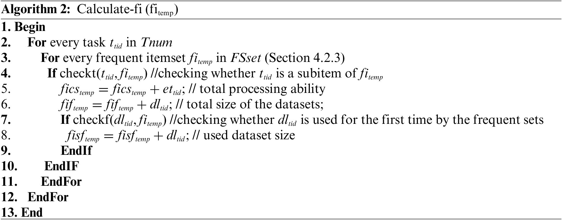
Algorithm 2 outputs the values of ficstemp, fiftemp, fisftemp. We can lay out the dataset and tasks in frequent itemsets according to these three values using Algorithm 3. For the frequent itemsets in FSset (Section 4.2.3), we have the following target:

Minimizing:

TS=∑fisftemp(18)

Subject to:

∀cid:∑checkc(temp,cid)fiftemp≤hccid(19)

∀cid:∑checkc(temp,cid)ficstemp≤pcid(20)

Formula (18) is the required size of the datasets of all tasks. Formulas (16) and (17) ensure that the hard disks and the CPU are not overloaded.

Formula (18) can also be expressed as follows:

TS=∑checkc(temp,cid)ficstemp−SFI(21)

SFIis the total size of the dataset in frequent itemsets (not all tasks). SFI is a constant, so the target function becomes

TS=∑checkc(temp,cid)ficstemp(22)

According to Formulas (18), (21), and (22), the dataset layout problem becomes a 0–1 programming problem. Algorithm 3 presents the data layout method in detail. In Formulas (21) and (22), function checkc(temp,cid) checks whether the dataset in the frequent itemset fitemp is located in cloud cid. In this paper, we suppose that the dataset in a frequent itemset has at least one cloud that can support its hard disk and processing requirements.

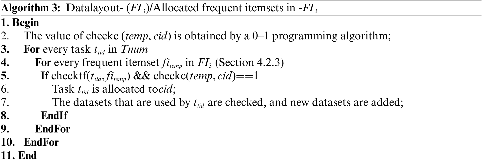
After that, we lay out other datasets and schedule meteorological models according to FI1 and FI2. We always try to lay out datasets in the frequent itemset of FI2 in a cloud (Lines 2~11, Algorithm 4; same as in the following paper). In addition, we also try to schedule meteorological models to the cloud that has the maximum percentage of the same dataset using the meteorological models (Lines 12~21). In Line 3, maxsize1 records the maximum percentage of the dataset in the frequent itemset fitemp that is located in the cloud cid. slecid1 records the unique identifier of the selected cloud. Lines 4~9 search for a cloud that satisfies our requirement (maximum percentage of the dataset). Line 9 lays out the dataset in the selected cloud. In Line 13, maxsize2 records the maximum percentage that a cloud can provide for the meteorological model, and slecid2 is the selected cloud. Lines 13~20 select a cloud for every meteorological model in FI1 by calculating the maximum percentage of datasets of a meteorological model in every cloud.

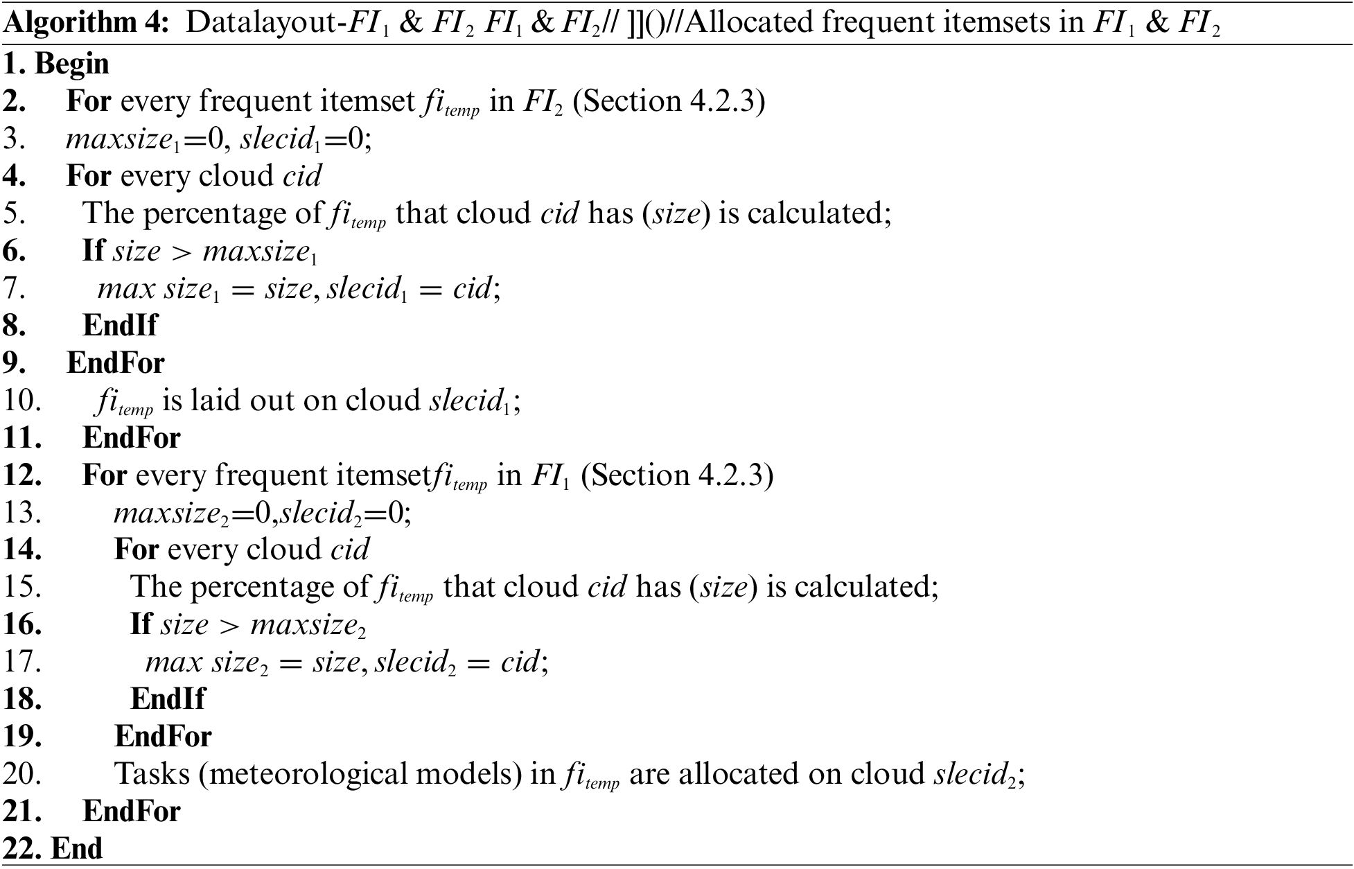
After we have laid out the datasets in FI2 and FI3 and have scheduled meteorological model tasks in FI1 and FI3, we can lay out other datasets and schedule other meteorological tasks. We just lay those datasets out in a cloud while ensuring that the processing ability (CPUs) of the cloud is not exceeded. Because the volume of hard disks in a cloud is always sufficient (compared to CPUs), we do not discuss them in detail here; we must ensure that there is at least one copy of every dataset. For the meteorological model tasks, we apply a max-max policy: for every task, we check each cloud to determine whether it has the maximum percentage (according to volume) of datasets that the task needs, and then we select the task that has the maximum percentage for all tasks. In Line 4 (Algorithm 5; same as in the following), mins is the maximum percentage of the datasets needed by Ttid that is located in Ctid, slecid is the selected cloud, and sletid is the selected task. Lines 3~10 attempt to find a suitable mapping between the task and cloud that satisfies the max-max policy by iterative searching. Line 11 allocates task sletid to cloud slecid.

5.3 Complexity Analysis

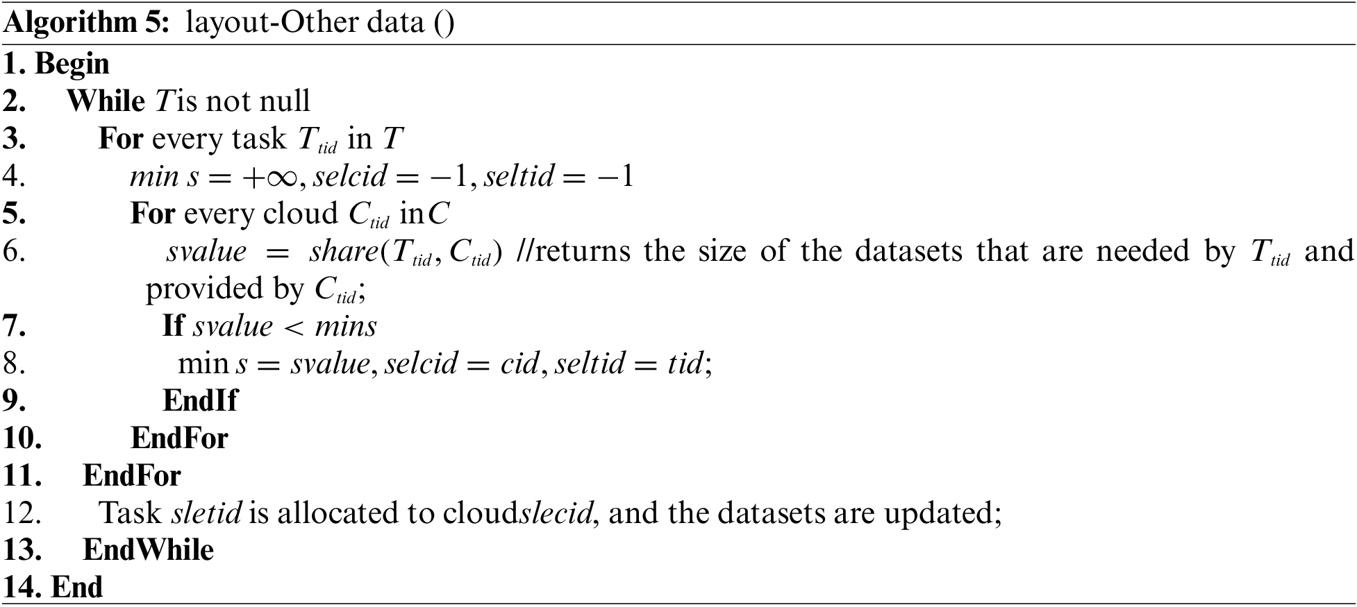
Because we can get the relations in Section 4 before execution, so, we do not take into account the complexity of algorithms in Section 4. So, the complexity of our method is decided by Algorithms 2~5.

Suppose F1, F2 and F3 have the number of frequent itemsets N1, N2 and N3, the number of clouds, tasks are Cnum and Tnum, then the complexity of Algorithms 2~5:

O(Algorithm 2)=Tnum∗(N1+N2+N3)(23)

O(Algorithm 3)=Tnum∗N3(24)

O(Algorithm 4)=Cnum∗(N1+N2)(25)

O(Algorithm 5)=Tnum∗Cnum(26)

So, the complexity of our method is:

O(FP)=Tnum∗(N1+N2+N3)+Cnum∗(N1+N2)+Tnum∗Cnum(27)

6  Simulations and Comparisons

In this section, we compare different data layout methods in terms of the average number of involved clouds (ANIC), the average size of files that are transferred between clouds (ASC), the average time for transferring files (ATTF), the rate of data that the task (ART) located on the cloud that the task assigned to, Average energy consumption for transferring files (AEC) and Average Execution Time of Various methods (AET). Those parameters can prove the efficiency of our method from different views. If our method has a lower value in ATTF, ANIC, ASC, AET, AEC, and a higher value in ART, this means our method has a good performance in the simulation environment.

6.1 Simulation Environment

The dataset in Table 1 has been laid out using our proposed FP-Growth-M method. The bandwidth between clouds is random in [100,500] M/s with uniform distribution, and the size of a dataset is random in [0~6] T with uniform distribution. We randomly generate a task in Table 1. We generate 10000 tasks by randomly selecting a record in Table 1, and every dataset has a 1%~5% possibility of being in the record. For all the compared metrics, the average values of 10000 execution times are reported. The power consumption for sending data and receiving data was 0.1W and 0.05W. The number of instructions is a random number in [102, 105] MIs (Million instructions). The processing ability of one core in the CPU is 2.3 GHz (According to the standard VM of a VMware center) and one CPU has 8 cores.

We will compare our method with Data-Aware [35–37] and Tran-Aware [38]. Data-Aware prefetches datasets that will be used by the meteorological model task. Tran-Aware clusters datasets together that have a higher possibility of being used together. In the simulation environment, there are four clouds. We will evaluate these methods under the condition that every cloud is 0.3~0.65 times the size of all datasets, with a step size of 0.05.

6.2 Comparisons and Discussions

6.2.1 Average Number of Involved Clouds

Fig. 4 presents the ANIC as a function of the hard disk size of each cloud. Generally, all methods show a decreasing trend with the increasing hard disk size of each cloud. FP-Growth-M has the lowest ANIC value for all cloud hard disk sizes. Tran-Aware first performs better than Data-Aware and then has almost the same performance as Data-Aware in terms of ANIC. Compared to the ANIC values of Data-Aware and Tran-Aware, the FP-Growth-M average ANIC value is lower by 6.23% and 8.97%, respectively. FP-Growth-M has the lowest ANIC value because it considers the relationships between meteorological models and meteorological datasets, which reduces the possibility that a meteorological model requires a dataset in a remote cloud.

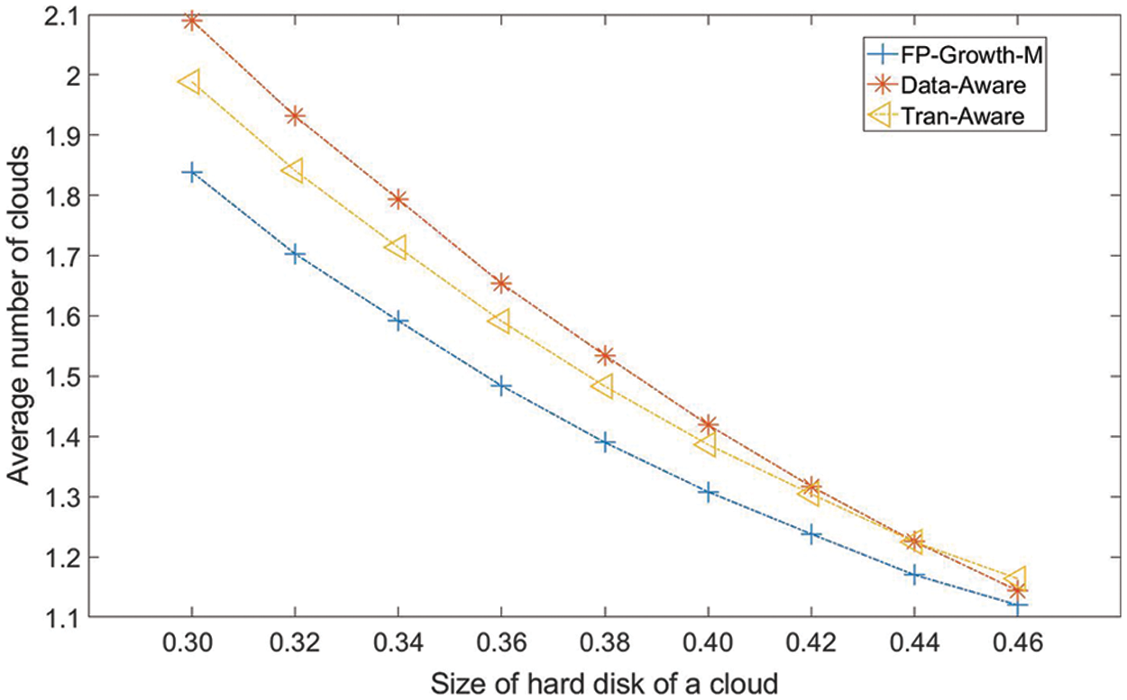
Figure 4: Average number of involved clouds

6.2.2 Average Size of the Files Transferred between Clouds

Fig. 5 presents the ASC values of FP-Growth-M, Tran-Aware, and Data-Aware for various cloud hard disk sizes. All three methods show drops in ASC as the size of the hard disk of each cloud increases. This is because as the size of the hard disk of each cloud increases, each cloud has more room for all the datasets that are required by the meteorological model task that is assigned to the cloud, which reduces the value of ASC. FP-Growth-M has the lowest value of ASC, followed by Tran-Aware and Data-Aware. Compared to the ASC values of Tran-Aware and Data-Aware, the FP-Growth-M average value is reduced by 17.87% and 31.08%, respectively.

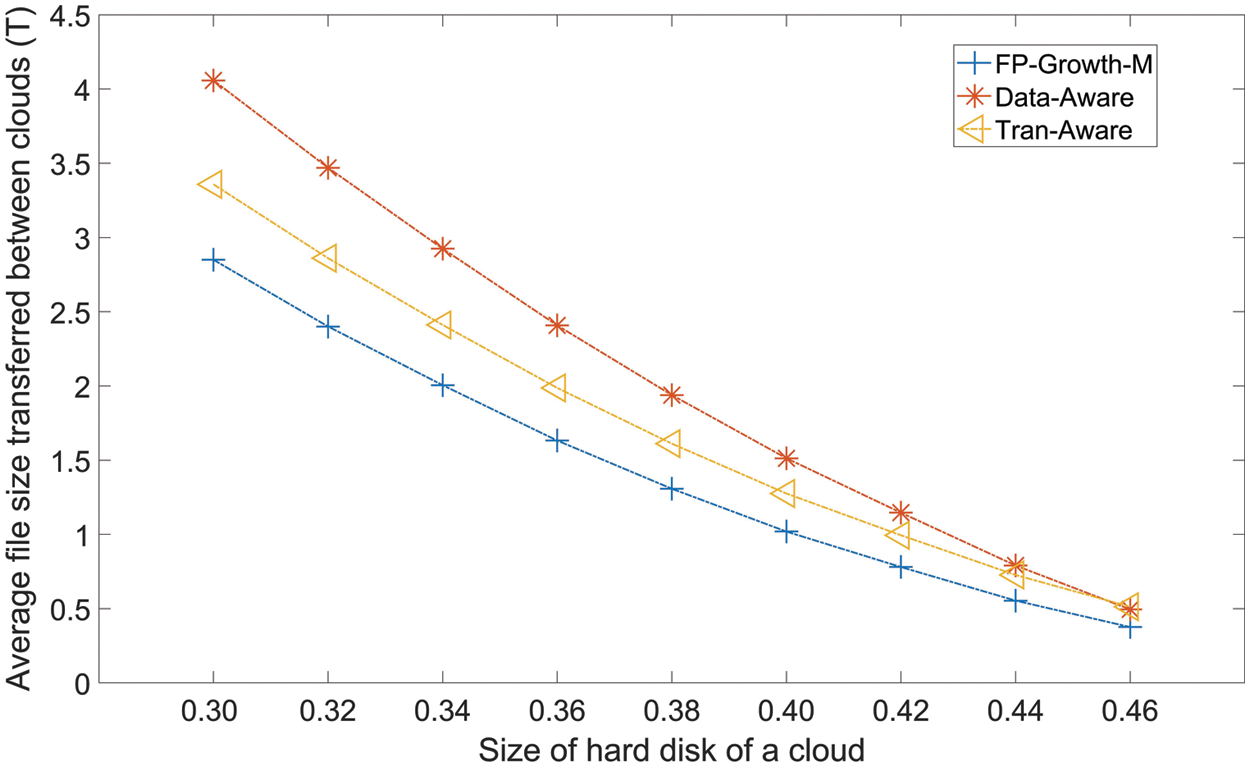
Figure 5: Average size of the files that transferred between clouds

6.2.3 Average Time for Transferring Files Between Clouds

Fig. 6 presents the ATTF values of the three methods versus the hard disk size of each cloud. These three methods have the same trend as for ANIC in Fig. 4. All methods show a decreasing trend with the enhancement of hard disk size of each cloud. FP-Growth-M has the lowest value of ATTF, followed by Tran-aware and Data-Aware. The trend of ATTF is the same as the trends of ANIC in Fig. 4 and ASC in Fig. 5. A larger value of ASC always results in a larger value of ATTF. Compared to the ATTF values of Tran-aware and Data-Aware, the FP-Growth-M average value is lower by 20.89% and 33.86%, respectively.

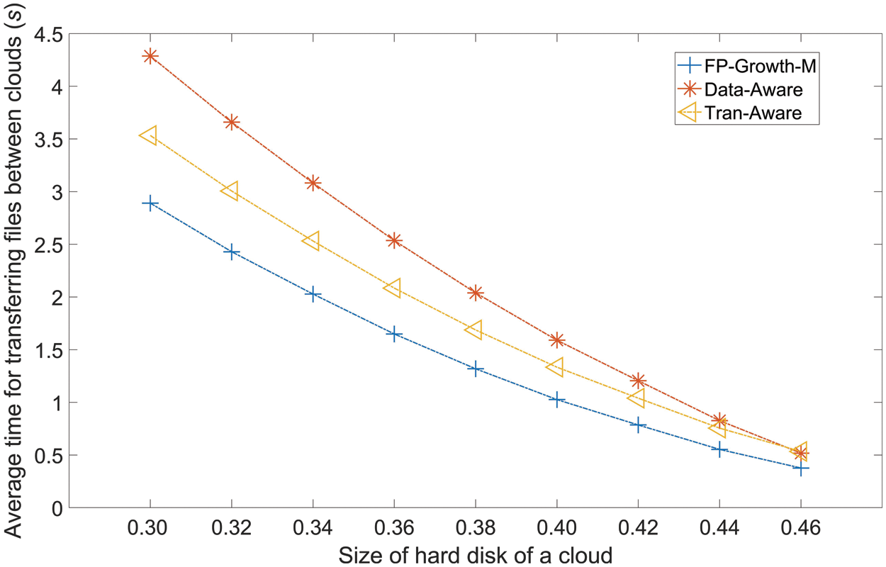
Figure 6: Average time for transferring files between clouds

6.2.4 The Rate of Data from Local Clouds

Fig. 7 gives the rate of data that the task (ART) located on the cloud that the task was assigned to. Generally, all methods have a descending trend with the enhancement of the size of the local hard disks. FP-Growth-M always has the highest rate, followed by Tran-Aware and Data-Aware. The average rate of FP-Growth-M, Tran-Aware, and Data-Aware are 41.89%, 36.04% and 29.76%. To the rate of Tran-Aware and Data-Aware, FP-Growth-M average enhances about 5.85% and 12.13%.

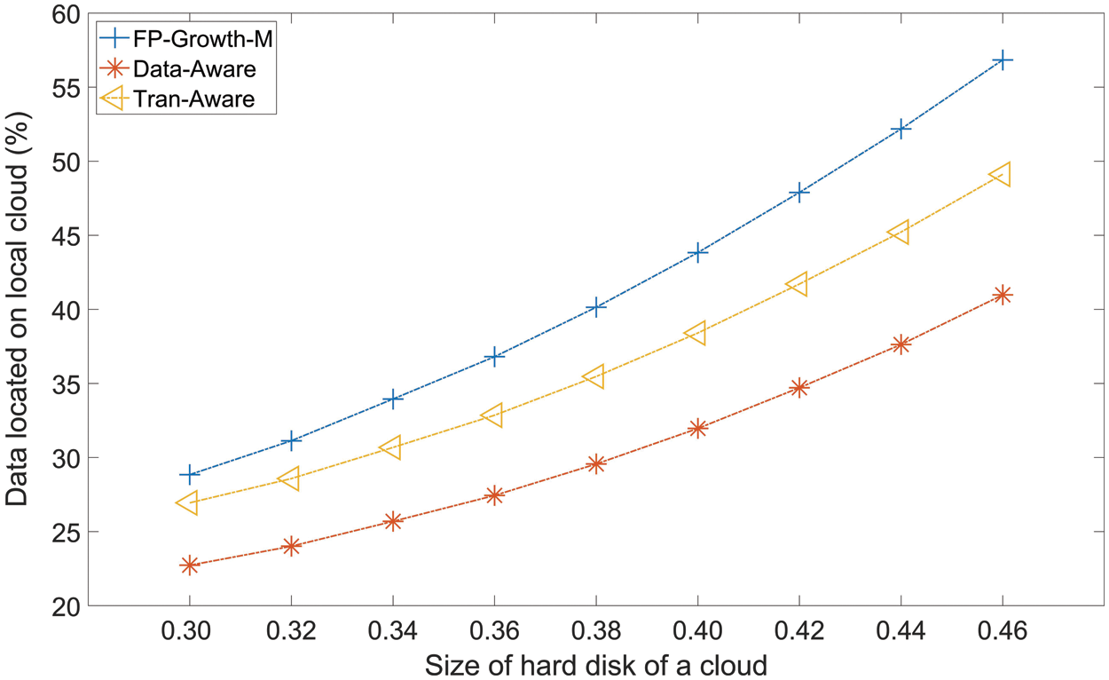
Figure 7: The average rate of data located on local cloud

6.2.5 Average Energy Consumption for Transferring Files

Fig. 8 is the AEC of different methods under different volume of hard disks. Generally speaking, the three methods both have a decreasing trend with the enhancement of the size of hard disks. Fp-Growth-M always has the lowest value in AEC, followed by Tran-Aware and Data-Aware. Compared to AEC of Tran-Aware and Data-Aware, Fp-Growth-M average decreases by 21.83% and 44.25%. Fig. 8 has the same trend to the data in Fig. 5 and Fig. 6. For the three methods, with the enhancement of data transferring between clouds (Fig. 5), more time (Fig. 6) and more energy consumption (Fig. 8) for transferring files.

Figure 8: Average energy consumption for transferring files

6.2.6 Average Execution Time of Various methods

Fig. 9 gives the AET of the three methods when the size of hard disks is changed from 0.30 to 0.46 with a step of 0.2. All methods have a decreasing trend when the size of hard disks is increased. To AET of Tran-Aware and Data-Aware, Fp-Growth-M average reduces 0.7533 and 0.3860.

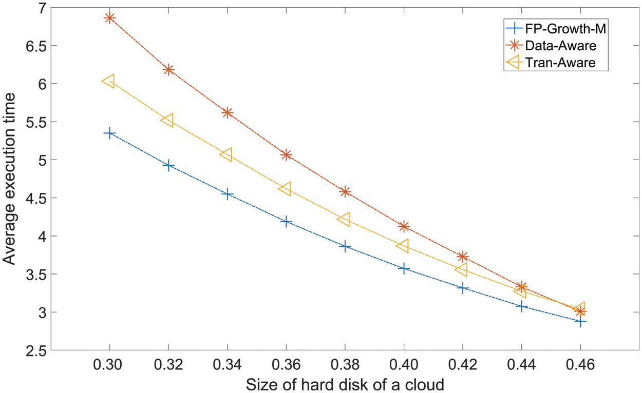
Figure 9: Average execution time

Generally, FP-Growth-M performs best among the three methods in terms of ANIC, ASC, ATTF, ART. FP-Growth-M has the best performance because it considers the relationships between meteorological models and meteorological datasets, thereby reducing the possibility that a meteorological model task needs to read a dataset in a remote cloud, which reduces the value of ANIC (Fig. 4). Considering the relationships between the inter datasets and meteorological models, we further reduce the time for obtaining data from a remote cloud (Fig. 6) and the sizes of the datasets from other clouds (Fig. 5); at the same time, it enhances the rate of data located on the local cloud (tasks and datasets located on the same cloud). Fp-Growth-M also has the lowest value in AET and AEC. Data-Aware sometimes may drop datasets that have a higher possibility of being used in the future if those datasets were not required recently, which increases the values of ANIC, ASC, and ATTF. Similar to Tran-Aware, it also clusters datasets according to their use over a short time period in the past, and it may remove some datasets that are used by most of the meteorological model tasks that are assigned to the cloud, thereby improving the values of ANIC, ASC, ATTF, AEC, and AET.

7  Conclusions and Future Work

In this paper, we investigate the meteorological data layout and meteorological task scheduling. We try to find the relation between meteorological model tasks and meteorological data sets. The incidence relation helps us to overcome transferring files between various clouds. Based on an analysis of the meteorological model task scheduling log, we used the FP-Growth method to mine the relationships (1) between meteorological model tasks, (2) between meteorological datasets, and (3) between meteorological model tasks and meteorological datasets. Based on these relationships, we proposed a heuristic algorithm method, FP-Growth-M, for scheduling meteorological model tasks and laying out meteorological datasets. Simulation results showed that the FP-Growth-M method reduces the time of transferring files between clouds and the related time. FP-Growth-M has the lowest value of the number of involved clouds. It also has the highest rate of data located on the local cloud. This means our proposed method can help us to lay out meteorological datasets to avoid data transferring between clouds, at the same time, it saves energy and time of execution tasks. Our model is based on a real meteorological system. The proposed method would help us lay out meteorological data sets for the real meteorological data layout. Furthermore, according to the data layout, we can schedule meteorological tasks more efficiently.

Because of the higher complexity of FP-Growth method, we may use some new cluster methods to reduce the complexity. Some new clustering methods [38,39] also have been used in different areas, we may use some of them to cluster our meteorological data sets and the meteorological tasks. In future work, we may also pay attention to improving the profit of the meteorological cloud center [40], and reducing the cost [41]. Now, The energy consumption of calculation shows explosive growth, especially in big data and cloud environments [5,6,42]. In future work, we may focus on energy-aware meteorological dataset layout and energy-aware meteorological model task scheduling and targets to reduce energy consumption during meteorological task execution. Because our method is only evaluated in a simulation environment, in future work, we may collect enough data to evaluate our method, and also give some support to other researchers.

Funding Statement: This research was funded in part by Major projects of the National Social Science Fund (16ZDA054) of China, the Postgraduate Research & Practice Innovation Program of Jiansu Province (NO. KYCX18_0999) of China, the Engineering Research Center for Software Testing and Evaluation of Fujian Province (ST2018004) of China.

Conflicts of Interest: The authors declare that they have no conflicts of interest to report regarding the present study.

References

1. B. Sliwa, R. Adam and C. Wietfeld, “Client-based intelligence for resource efficient vehicular big rata transfer in future 6G networks,” IEEE Transactions on Vehicular Technology, vol. 70, no. 6, pp. 5332–5346, 2021. [Google Scholar]

2. E. A. Abir, P. K. Sharma and J. H. Park, “Blockchain-based delegated Quantum Cloud architecture for medical big data security,” Journal of Network and Computer Applications, vol. 198, no. 2, pp. 1–13, 2022. [Google Scholar]

3. Q. Xia, Z. Xu, W. Liang and A. Y. Zomaya, “Collaboration- and fairness-aware big data management in distributed clouds,” IEEE Transaction Parallel Distribution System, vol. 27, no. 7, pp. 1941–1953, 2016. [Google Scholar]

4. R. D. March, C. Leuzzi, M. Deffacis, F. Caronte, A. F. Mulone et al., “Innovative approach for PMM data processing and analytics,” IEEE Transaction Big Data, vol. 6, no. 3, pp. 452–459, 2020. [Google Scholar]

5. R. Tudoran, A. Costan and G. Antoniu, “OverFlow: Multi-site aware big data management for scientific workflows on clouds,” IEEE Transaction Cloud Computing, vol. 4, no. 1, pp. 76–89, 2016. [Google Scholar]

6. Z. Haiyun and X. Yizhe, “Microprocessors and microsystems sports performance prediction model based on integrated learning algorithm and cloud computing Hadoop platform,” Microprocessors and Microsystems, vol. 79, no. 11, pp. pp 1–7, 2020. [Google Scholar]

7. K. Kalia and N. Gupta, “Analysis of hadoop MapReduce scheduling in heterogeneous environment,” Ain Shams Engineering Journal, vol. 12, no. 1, pp. 1101–1110, 2021. [Google Scholar]

8. S. Fiore, D. Elia C. E. Pires, D. G. Mestre and G. Aloisio, “An Integrated big and fast data analytics platform for smart urban transportation management,” IEEE Access, vol. 7, pp. 117652–117677, 2019. [Google Scholar]

9. H. A. Owolabi, M. Bilal, L. O. Oyedele, H. A. Alaka, S. O. Ajayi et al., “Predicting completion risk in PPP projects using big data analytics,” IEEE Transactions on Engineering Management, vol. 67, no. 2, pp. 430–453, 2020. [Google Scholar]

10. H. Balti, A. B. Abbes, N. Mellouli, I. R. Farah, Y. Sang et al., “A review of drought monitoring with big data: Issues, methods, challenges and research directions,” Ecological Informatics, vol. 60, no. August, pp. 1–17, 2020. [Google Scholar]

11. R. Tripathi, R. S. Mazmudar, K. D. Knusel, J. S. Bordeaux and J. F. Scott, “Big data in dermatology: Publicly available health care databases for population health research,” Journal of the American Academy of Dermatology, vol. 83, no. 5, pp. 1546–1556, 2020. [Google Scholar] [PubMed]

12. L. Zheng, J. Yang, L. Chen, D. Sun and W. Liu, “Dynamic spatial-temporal feature optimization with ERI big data for short-term traffic flow prediction,” Neurocomputing, vol. 412, no. 1, pp. 339–350, 2020. [Google Scholar]

13. L. Kong, Z. Liu and J. Wu, “A systematic review of big data-based urban sustainability research: State-of-the-science and future directions,” Journal of Cleaner Production, vol. 273, no. 11, pp. 123–142, 2020. [Google Scholar]

14. W. Tian, L. Yi, W. Liu, W. Huang, G. Ma et al., “Ground radar precipitation estimation with deep learning approaches in meteorological private cloud,” Journal of Cloud Computing, vol. 9, no. 1, pp. 1–12, 2020. [Google Scholar]

15. Y. Hao, L. Wang and M. Zheng, “An adaptive algorithm for scheduling parallel jobs in meteorological cloud,” Knowledge-Based System, vol. 98, no. 4, pp. 226–240, 2016. [Google Scholar]

16. A. Quarati, E. Danovaro, A. Galizia, A. Clematis, D. D.' Agostino et al., “Scheduling strategies for enabling meteorological simulation on hybrid clouds,” Journal of Computational & Applied, vol. 273, no. 1, pp. 438–451, 2015. [Google Scholar]

17. W. Shu, K. Cai and N. N. Xiong, “Research on strong agile response task scheduling optimization enhancement with optimal resource usage in green cloud computing,” Future Generation Computer Systems, vol. 124, no. 11, pp. 12–20, 2021. [Google Scholar]

18. N. Moustafa and V. Tamarapalli, “Towards cost-aware VM migration to maximize the profit in federated clouds,” Future Generation Computer Systems, vol. 134, no. 3, pp. 53–65, 2022. [Google Scholar]

19. N. Gholipour, E. Arianyan and R. Buyya, “A novel energy-aware resource management technique using joint VM and container consolidation approach for green computing in cloud data centers,” Simulation Modelling Practice and Theory, vol. 104, no. 11, pp. 1–15, 2020. [Google Scholar]

20. A. Javadpour and A. Wang, “CTMvSDN: Improving resource management using combination of Markov-process and TDMA in software-defined networking,” Journal of supercomputing, vol. 78, no. 3, pp. 3477–3499, 2022. [Google Scholar]

21. A. Jayanetti, S. Halgamuge and R. Buyys, “Deep reinforcement learning for energy and time optimized scheduling of precedence-constrained tasks in edge-cloud computing environment,” Future Generation Computer Systems, vol. 137, no. 6, pp. 14–30, 2022. [Google Scholar]

22. H. Song, Y. Yin, Y. Chen and X. H. Sun, “Cost-intelligent application-specific data layout optimization for parallel file systems,” Cluster Computing, vol. 16, no. 2, pp. 285–298, 2013. [Google Scholar]

23. K. A. Zaman and S. Padmanabhan, “An efficient workload-based data layout scheme for multidimensional data,” Data & Knowledge Engineering, vol. 39, no. 3, pp. 271–291, 2001. [Google Scholar]

24. I. Suh and Y. D. Chung, “DimensionSlice: A main-memory data layout for fast scans of multidimensional data,” Information System, vol. 94, no. 12, pp. 1–14, 2020. [Google Scholar]

25. J. Zhou, H. Wu and J. Wang, “ApproxSSD: Data layout aware sampling on an array of SSDs,” IEEE Transaction Computers, vol. 68, no. 4, pp. 471–483, 2019. [Google Scholar]

26. J. D. Booth, N. D. Ellingwood, H. K. Thornquist and S. Rajamanickam, “Basker: Parallel sparse LU factorization utilizing hierarchical parallelism and data layouts,” Parallel Computing, vol. 68, no. 2, pp. 17–31, 2017. [Google Scholar]

27. O. Bel, K. Chang, R. T. Nathan and D. Duellmann, “Geomancy: Automated performance enhancement through data layout optimization,” in IEEE Int. Symp. on Performance Analysis of Systems and Software, Boston, MA, USA, pp. 119–120, 2020. [Google Scholar]

28. Z. Liu, T. Xiang, B. Lin, X. Ye, H. Wang et al., “A data placement strategy for scientific workflow in hybrid cloud,” in IEEE 11th Int. Conf. on Cloud Computing, San Francisco, CA,USA, pp. 556–563, 2018. [Google Scholar]

29. Y. Jiang, X. Liu, Y. H. Li and Y. Zhang, “A data layout method suitable for workflow in a cloud computing environment with speech applications,” International Journal of Speech Technology, vol. 24, no. 1, pp. 31–40, 2020. [Google Scholar]

30. C. Ji, F. Wu, Z. Zhu, L. P. Chang, H. Liu et al., “Memory-efficient deep learning inference with incremental weight loading and data layout reorganization on edge systems,” Journal of Systems Architecture, vol. 118, no. 7, pp. 1–9, 2021. [Google Scholar]

31. Y. Hao, J. Cao, T. Ma and S. Ji, “Adaptive energy-aware scheduling method in a meteorological cloud,” Future Generation Computer Systems, vol. 101, no. 7, pp. 1142–1157, 2019. [Google Scholar]

32. Y. He and D. Fengdong, “Design and implementation of meteorological big data platform based on hadoop and elasticsearch,” in IEEE 4th Int. Conf. on Cloud Computing and Big Data Analytics, Chengdu, China, pp. 705–710, 2019. [Google Scholar]

33. M. Yang, W. He, Z. Zhang, Y. Xu, Y. Chen et al., “An efficient storage service method for multidimensional meteorological data in cloud environment,” in Int. Conf. on Internet of Things (iThings) and IEEE Green Computing and Communications (GreenCom) and IEEE Cyber, Physical and Social Computing (CPSCom) and IEEE Smart Data (SmartData), Atlanta, GA, USA, pp. 495–500, 2019. [Google Scholar]

34. F. Ruan, R. Gu, T. Huang and S. Xue, “A big data placement method using NSGA-III in meteorological cloud platform,” EURASIP Journal on Wireless Communications, vol. 2019, no. 1, pp. 1, 2019. [Google Scholar]

35. Y. Li, W. Xia, Y. Huang, J. Shao and Z. Shu, “Research on stream data clustering based on swarm intelligence,” in Proc. of 2011 Int. Conf. on Computer Science and Network Technology, Harbin, China, pp. 573–577, 2021. [Google Scholar]

36. P. Kasu, T. Kim, J. H. Um, K. Park, S. Atchley et al., “Object-logging based fault-tolerant big data transfer system using layout aware data scheduling,” IEEE Access, vol. 7, pp. 37448–37462, 2019. [Google Scholar]

37. K. A. Zaman and S. Padmanabhan, “An efficient workload-based data layout scheme for multidimensional data,” Data & Knowledge Engineering, vol. 39, no. 3, pp. 271–291, 2001. [Google Scholar]

38. M. Lee and Y. I. Eom, “Transaction-aware data cluster allocation scheme for Qcow2-based virtual disks,” in IEEE Int. Conf. on Big Data and Smart Computing (BigComp), Busan, Korea(Southpp. 385–388, 2020. [Google Scholar]

39. P. S. Rathore and B. K. Sharma, “Improving healthcare delivery system using business intelligence,” Journal of IoT in Social, Mobile, Analytics, and Cloud, vol. 4, no. 1, pp. 11–23, 2022. [Google Scholar]

40. P. Cong, X. Hou, M. Zou, J. Dong, M. Chen et al., “Multiserver configuration for cloud service profit maximization in the presence of soft errors based on grouped grey wolf optimizer,” Journal of Systems Architecture, vol. 127, no. 12, pp. 1–12, 2022. [Google Scholar]

41. S. Chen, J. Liu, F. Ma and H. Huang, “Customer-satisfaction-aware and deadline-constrained profit maximization problem in cloud computing,” Journal of Parallel and Distributed Computing, vol. 163, no. 21, pp. 198–213, 2022. [Google Scholar]

42. Y. Hao, J. Cao, Q. Wang and J. Du, “Energy-aware scheduling in edge computing with a clustering method,” Future Generation Computer Systems, vol. 117, no. 5, pp. 259–272,2021, 2021. [Google Scholar]