
 Submit a Paper
 Propose a Special lssue
 Open Access
ARTICLE

Intelligent Fish Behavior Classification Using Modified Invasive Weed Optimization with Ensemble Fusion Model
School of Computing, Sathyabama Institute of Science and Technology, Chennai, 600 119, India
* Corresponding Author: B. Keerthi Samhitha. Email:
Intelligent Automation & Soft Computing 2023, 37(3), 3125-3142. https://doi.org/10.32604/iasc.2023.040643
Received 26 March 2023; Accepted 17 May 2023; Issue published 11 September 2023
 View Full Text
 Download PDF
Abstract
Accurate and rapid detection of fish behaviors is critical to perceive health and welfare by allowing farmers to make informed management decisions about recirculating the aquaculture system while decreasing labor. The classic detection approach involves placing sensors on the skin or body of the fish, which may interfere with typical behavior and welfare. The progress of deep learning and computer vision technologies opens up new opportunities to understand the biological basis of this behavior and precisely quantify behaviors that contribute to achieving accurate management in precision farming and higher production efficacy. This study develops an intelligent fish behavior classification using modified invasive weed optimization with an ensemble fusion (IFBC-MIWOEF) model. The presented IFBC-MIWOEF model focuses on identifying the distinct kinds of fish behavior classification. To accomplish this, the IFBC-MIWOEF model designs an ensemble of Deep Learning (DL) based fusion models such as VGG-19, DenseNet, and EfficientNet models for fish behavior classification. In addition, the hyperparameter tuning of the DL models is carried out using the MIWO algorithm, which is derived from the concepts of oppositional-based learning (OBL) and the IWO algorithm. Finally, the softmax (SM) layer at the end of the DL model categorizes the input into distinct fish behavior classes. The experimental validation of the IFBC-MIWOEF model is tested using fish videos, and the results are examined under distinct aspects. An Extensive comparative study pointed out the improved outcomes of the IFBC-MIWOEF model over recent approaches.Keywords
The demand for aquatic products has significantly increased over the past 20 years due to the world population’s fast growth [1]. Many countries’ principal source of fishery products has shifted to fish farming due to the rapidly increasing demand for aquatic goods. However, the lack of efficient fish health and management practices and welfare monitoring is causing this industry to suffer tremendous losses on a global scale [2]. Animals frequently engage in complex interactions with one another and with their environment. Tools that measure behavior automatically and simultaneously provide in-depth knowledge of the relationship between the external environment and behavior are required since it is possible to distinguish behavioral activities from video files [3]. In fish farming research, how the yield and efficiency can be improved turns out to be a significant problem, and this becomes a severe issue that should be sorted out that limits the growth of the aquaculture sector [4]. The premise for solving this issue is obtaining the fish’s behavior analysis via the behavior trajectory, identifying the irregularities and rules to guide the breeding and thwart the occurrence of abnormal conditions [5].
To proceed with the fish behavior analysis, the location and recognition become essential for the fish after examining the fish’s behavior. Currently, the prevailing techniques for analysis and recognition are categorized into quantitative and qualitative methods [6]. Qualitative techniques have three types. Firstly, the complete manual approaches for analysis and recognition, like the manual marking technique or manual observation approach. Secondly, the fluorescent-related credit and manual analysis approach employed fluorescent markers to locate the fish and physically analyze the behavior [7]. Thirdly the video-related award and manual analysis approach. Thirdly, a feature was put into the fish’s body, and the video was utilized for tracking the marker in the fish’s body. This approach so far requires physical behavior analysis for fish [8]. The following two types of techniques were all invasive; thus, such techniques results in the stress behavior of fish, and the behavior analysis only is performed manually. These methods were laborious and time-consuming, and the behavior analysis outcomes were vulnerable to subjective elements. In addition, only the qualitative effects are acquired instead of the quantitative results, and the behavior trajectory may not be plotted.
To make a solution to the issue, the subjective elements can influence the manual analysis, and the quantitative outcomes may not be attained; the quantitative approaches were suggested for analyzing the fish behavior. The quantitative methods have two kinds. One is related to appearance features for recognizing the objects and obtaining the behavior trajectory, like infrared reflection and shape matching [9]. Another is related to image processing for identifying objects and obtaining the behavior trajectory, like the optical flow method and inter-frame difference technique. Introducing the Computer Vision (CV) approach in aquaculture has created new options for accurately and efficiently observing fish behavior. Conventional CV methods to identify fish behavior depend on deriving significant features, namely trajectory, motion patterns, and clustering index [10]. Deep learning (DL) techniques have revolutionized the ability to mechanically examine videos utilized for live fish identification, water quality monitoring, species classification, behavior analysis, and biomass estimation. The benefit of DL is it can mechanically learn to extract image features and exhibits remarkable performance in identifying sequential activities.
Deep learning algorithms have produced accurate target detection and tracking. However, it is still necessary to create strategies for recognizing fish behavior to consider the complex underwater environment and swift target movement. In reaction to environmental stimuli, fish typically alter their swimming technique. Due to the chance that two dissimilar kinds of activities in a video sequence display comparable activity, the success probability of recognition is lowered. For instance, both eating exercise and threatening behavior involve fish moving quickly after being aroused. An extensive range of various activity states is also included in one category of behavior. For instance, hypoxic fish are sinking on the tank’s side and actively congregating there. Therefore, tiny alterations among dissimilar behavior categories and frequent samples of the similar action pose the biggest obstacles to implementing deep learning in fish behavior identification.
This study proposes an IFBC-MIWOEF model that uses temporal and spatial feature information to read a school of fish’s behavior states from video data to overcome the abovementioned challenges. Our work has made the following main contributions: (1) An innovative method for detecting fish activity based on deep learning. (2) The proposed framework combines the RGB and optical flow image elements to identify the five fish behaviors. (3) The suggested framework exhibits good performance and acceptable outcomes. By automatically identifying fish behavior in real-time from video clips using our suggested method, we lay the framework for aquaculture to develop into a more intelligent industry.
This study develops an intelligent fish behavior classification using modified invasive weed optimization with an ensemble fusion (IFBC-MIWOEF) model. The IFBC-MIWOEF model’s recognition and classification of various types of fish behavior is one of its main objectives. Primarily, the input videos are collected, and the frame conversion process takes place. The VGG-19, DenseNet, and EfficientNet models also employ a fusion-based feature extraction method. Additionally, the IWO algorithm and OBL concept are combined to create the MIWO algorithm, which is used to tune the hyperparameters of the DL models. Further, the input is divided into various fish behavior classes by the softmax (SM) layer after the DL model. Several simulations utilizing various measures were run to show the effectiveness of the IFBC-MIWOEF model.
A thorough analysis of the models for categorizing fish behavior is provided in this section. Iqbal et al. [11] provided an automatic mechanism for classifying and detecting fish. It is helpful for marine biologists to get a better understanding of their habitats and fish species. The presented method depends on Deep Convolutional Neural Networks (DCNN). It employs a minimized version of the AlexNet method and has two fully connected (FC) layers and four convolutional layers. A comparison was made with the other DL methodologies, namely AlexNet and VGGNet. Jalal et al. [12] projected a hybrid method combining Gaussian mixture methods and optical flow with YOLO Deep Neural Networks (DNN) to locate and categorize fish in unrestricted underwater footage. The YOLO-related object detection mechanism was initially used to capture just the static and visible fish. And removes this restriction of YOLO, enabling it to detect freely moving fish, invisible in the background, utilizing temporary data obtained through optical flow and Gaussian mixture methods.
For automatic fish species categorization, Tamou et al. [13] used transfer learning (TL) in conjunction with CNN AlexNet. The pre-trained AlexNet, either with or without finetuning, generates features from foreground fish photos of the existing underwater data set. Chhabra et al. [14] suggested a fish classifier system that functions in a natural underwater atmosphere to detect fishes with nutritional or medicinal significance. The article used a hybrid DL method, whereas the Stacking ensemble method was employed for detecting and classifying fishes from images, and a pre-trained VGG16 technique was utilized for Feature Extraction. According to [15], machine vision is offered to assess fish appetite, and CNN automatically scores fish feeding intensity. Following were the specific implementation steps. First, photos taken throughout the feeding process have been collected, and a data set has been expanded using noise-invariant data expansion and rotation, scale, and translation (RST) augmentation methods. Afterward, a CNN was trained over the trained data set, and the fish appetite level could be graded using the trainable CNN method.
Farooq et al. [16] proposed a novel method to identify unusual crowd behavior in surveillance footage. The main goal of this study is to identify crowd divergence behaviors that may result in dangerous scenarios like stampedes. We categorize crowd activity using a convolution neural network (CNN) trained on motion-shape images (MSIs), and we provide the potential for physically capturing motion in photographs. The finite-time Lyapunov exponent (FTLE) field is generated after the optical flow (OPF), which was initially determined, has been integrated. The coherent Lagrangian structure (LCS) represents crowd-dominant motion in the FTLE field. It is suggested to transform LCS-to-grayscale MSIs using ridge extraction. Not to mention that CNN has received supervised training to foresee divergence or typical behaviors for each unidentified image. Describe a deep-fusion model that utilizes the numerous convolutional layers of a deep neural network’s hierarchical feature exits effectively and efficiently in [17]. We specifically recommend a network that combines multiscale data from the network’s surface to deep layers to transform the input image into a density map. The final crowd size is calculated by adding the peaks on the density map. On the benchmark datasets UCF_CC_50, ShanghaiTech, and UCF-QNRF, experiments are conducted to evaluate the performance of the future deep network.
Alzahrani et al. [18] proposed a framework for a deep model that automatically classifies crowd behavior based on motion and appearance. This study first extracts dense trajectories from the input video segment and then projects those trajectories onto the image plane to generate the trajectory image. The trajectory image effectively depicts the scene’s relative motion. We employ a stack of trajectory images to teach a deep convolutional network a compact and potent representation of scene motion. Reference [19] proposed a technique for initializing a dynamical system described by optical flow, a high-level measure of overall movement, by superimposing a grid of particles over a scene. The dynamical scheme’s time integration generates brief particle trajectories (tracks), which reflect dense but transient motion designs in scene fragments. Then, trackless are expanded into longer routes, clustered using an unsupervised clustering technique, and compared for similarity using the longest common subsequence.
Knausgård et al. [20] published a two-step DL method to characterize temperate fishes without prefiltering. The primary stage is to identify every fish species, regardless of sex or species, that can be seen in the image. From now on, make use of the YOLO object detection technique. Each fish in the picture is classified in the second stage using a CNN without prefiltering and the Squeeze-and-Excitation (SE) structure. And uses Transfer Learning (TL) to progress the classifier’s performance and get around the poorly trained samples of temperate fish. A new image-related technique for fish identification was suggested by Revanesh et al. [21] to drastically reduce the number of undersized fish caught during commercial trawling. The suggestion concerns the trawl’s direct-located Deep Vision imaging mechanism’s acquisition of stereo images and processing those data. The pre-processing of the photos correctly accounted for the camera responses’ non-linearity. Afterward, each fish in the pictures may be localized and segmented using a Mask Recurrent Convolutional Neural Networks (RCNN) framework.
To identify and categorize various types of fish behavior, a novel IFBC-MIWOEF model has been established in this work. Primarily, the input videos are collected, and the frame conversion process takes place. Then, the fusion-based feature extraction process is carried out through three DL models, namely VGG-19, DenseNet, and EfficientNet. The performance of the DL algorithms can be improvised using the MIWO algorithm-based hyperparameter tuning process. The SM layer assigns the correct class labels to the input video frames at the very end. Fig. 1 portrays the block diagram of the IFBC-MIWOEF method.

Figure 1: Block diagram of IFBC-MIWOEF method
A collection of behavior films of fish of various sizes, times, and quantities can be collected over three months to conduct the experiment in the best possible way and verify the proposed technique’s effectiveness. Since fishes typically act in groups, every fish was photographed using the top camera [22]. The video is frequently downloaded into our computer from the memory card of network cameras and preserved there. In 24 h, several stages of fish behavior will be observed and recorded for the study. Other behaviors that are influenced by the environment, besides general behaviors like feeding, include fish startle stimulation, hypoxia, and hypothermia. They are categorized as hypothermia, eating, normal, hypoxic, and terrifying behaviors using expert experiences and talents.
3.2 Fusion Based Feature Extraction
The DL mechanisms are combined in the weighted voting-based ensemble approach, and the highest results are carefully selected using this method. Each vector is utilized for training the voting mechanism, and the fitness function (FF) is then used to determine the tenfold cross-validation accuracy. Consider the
Now,
Recently, many standard deep learning modules, like VGGNet, AlexNet, Inception, ResNet, Xception, DenseNet, and so on, have been utilized to detect plant disease. VGG network comprises multiple convolutional and pooling layers with various filter counts [23]. VGGNet consists of VGG16 and VGG19 modules. VGG16 has sixteen convolutional and pooling layers with the FC layer. VGG19 comprises nineteen convolutional and pooling layers with FC. The parameter count produced in the VGGNet is 140 million. The VGGNet is pre-trained on a larger dataset (ImageNet) with 1000 classes.
In this study, we employed shallow VGG module that takes nine layers of VGG19 that consist of 2
DenseNet is a network with many connections. Dense Blocks and Transition Layers are the two components that make up this structure. All levels in this network are directly connected in a feed-forward fashion. Prior layers’ feature maps are inputs for each layer. ReLU activation, 3 3 Convolution, and Batch Normalisation comprise a Dense Block. Between every two Dense Blocks are transition layers. These include Average Pooling, Batch Normalisation, and 1−1 Convolution. Each dense block’s feature maps are the same size for concatenation.
DenseNet is CNN, where every layer in the network is interconnected with each successive layer in a feedforward manner [24]. The input layer is a concatenation of feature map of each preceding layer. Specifically, for a network with
A DenseNet comprises
In Eq. (3),
The EfficientNet family’s EfficientNetB0 baseline network is recommended to have the lowest memory requirements while having the most excellent accuracy and FLOPS requirements feasible [25–27]. The network’s width and depth (number of channels and layers) can be changed, or the picture resolution can be raised so that the network can learn fine-grained features from the image. However, as this method includes dimensioning gain as scaling rises, multiple manual adjustments should be made to obtain an optimal match for each model. The EfficientNet family has emerged as a solution to the problem using the compound scaling strategy that the researcher provided. The method usages a multiple constant to uniform scaling network resolution, depth, and width.
In Eq. (4), the network depth is signified by the period, the network width is signified as
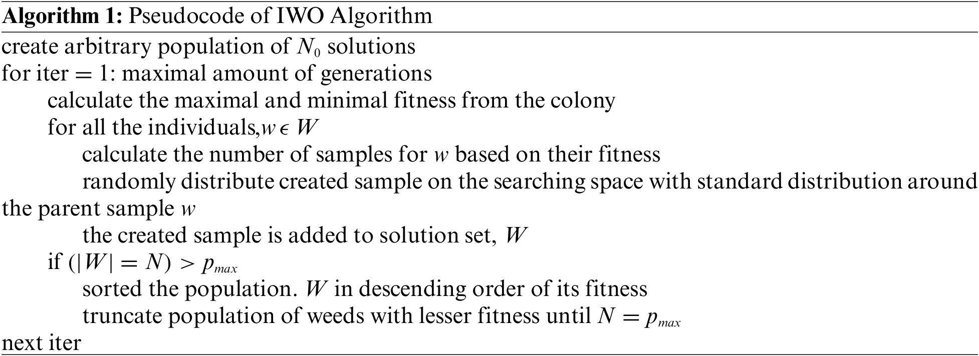
This study uses the MIWO technique to change the DL model hyperparameters in the best possible way. The IWO algorithm is a population-based optimization technique that finds a mathematical function by mimicking the randomness and compatibility of weed colonies [28–30]. Weed is one of the powerful herbs that aggressive growth habit provides a significant risk to the crops. It proves to be adaptable and very resistant to changes in the environment. As a result, considering its features, an effective optimization technique is accomplished. This approach tries to imitate a weed community’s randomness, resistance, and adaptability. This technique is based on the agricultural phenomenon named colonies of IWs. A plant is called a weed if it grows unintentionally in an area and obstructs human needs and activities, even though it may have other uses and benefits in some places. Mehrabian and Lucas 2006, developed a mathematical optimization algorithm inspired by the colonized weed named the “Invasive Weed Optimization (IWO) Algorithm.” Using essential weed colony characteristics, including growth, competition, and seeding, this method is efficient and straightforward in its convergence to the best solution [31–33].
To imitate the habitat behaviors of weeds, some key characteristics of the procedure are given in the following:
Initial populace: A limited number of seeds are discrete in the search space.
Reproduction: Each seed grows into a flowering plant that then releases another source, depending on the fitness levels. The number of grains of grass linearly reduces from
Spectral Spread: The seed generated by the group in the standard distribution with a standard deviation (SD) and mean planting location is generated using the following formula:
In Eq. (6), the number of maximum iterations can be represented as
This guarantees that the fall of grain in the variety reduces non-linearly at every stage, which eliminates unfitting plants and results in more appropriate plants and presentations of the transfer mode from to selection of
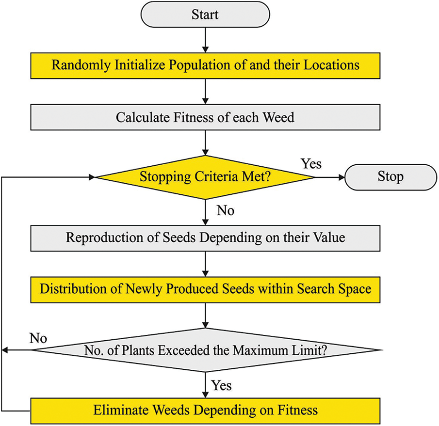
Figure 2: Flowcharts of IWO
Competitive deprivation: The herb population remains constant by removing the grass with the lowest fitness when the number of grasses in the colony reaches its maximum (Pmax). This process is done as often as necessary, and then the grass’s most minor colony cost function is saved. The oppositional-based learning (OBL) notion is used to compute the MIWO algorithm [34–36].
To improve the convergence speed and the possibility of defining the global optimum of the typical IWO technique [37–39], this work presents an improved version of the proposed method named the MIWO approach. During the primary iteration of the technique [40–42], afterward creating the immediate random solutions (that is, rats’ positions), the opposite places of all the answers are made dependent upon the model of the opposite number [43,44]. To describe the initialized novel population, it is necessary to determine the model of opposite numbers. Assume that
whereas
For applying the model of opposite numbers from the population initialized of AO technique, assume
The MIWO system generates an FF to enhance classifier presentation. It resolves a positive integer to indicate the higher version of the applicant outcomes. This study assumed that FF was provided in Eq. (9), which would reduce the classification error rate.
The feature extraction map is used to learn mappings between output classes and features that typically involve the FC layer and have each input from one layer connected with each activation unit of the succeeding layers. They are used in the network tail’s classification function, where a layer with many neurons matching several output classes is used. In a multiclass classification problem, the
In Eq. (10),
Three publicly available datasets, VGG-19, EfficientNet, and DenseNet, are used in this study to assess and associate the performance of the proposed framework with other existing methodologies. Pytorch was used to create the recommended network, and an NVIDIA Titan Xp GPU was used to train it. CUDA Toolkit 10.2, Pytorch 1.4, Anaconda 3, and Ubuntu 16.04 (64-bit) were all used in the test setup.
The experimental validation of the IFBC-MIWOEF technique is examined through several simulations. The dataset is represented in Table 1 as 5000 samples with five class labels.

The confusion matrices for classifying fish behavior produced by the IFBC-MIWOEF model are shown in Fig. 3. The IFBC-MIWOEF approach identified 788 samples under the FED class, 734 samples under the HYP class, 758 samples under the HYPOT class, 770 examples under the FRG class, and 771 examples under the NOR class with 80% of the TR dataset. Additionally, the IFBC-MIWOEF approach identified 679 samples under the FED class, 663 samples under the HYP class, 657 samples under the HYPOT class, and 681 samples under the FRG class 691 examples under the NOR class with 70% of the TR data. The IFBC-MIWOEF approach has also classified 290 examples under the FED class, 292 models under the HYP class, 281 samples under the HYPOT class, 295 under the FRG class, and 276 examples under the NOR class using only 30% of the TS data.


Figure 3: Confusion matrices of IFBC-MIWOEF approach (a) 80% of TR data, (b) 20% of TS data, (c) 70% of TR data, and (d) 30% of TS data
The consequences of the IFBC-MIWOEF model using 80% TR and 20% TS data are briefly presented in Table 2. On 80% of the TR dataset, Fig. 4 shows the general organization result of the IFBC-MIWOEF model. According to the figure, the IFBC-MIWOEF approach has shown improved outcomes across the board. For illustration, the IFBC-MIWOEF method has categorized examples under the FED class with

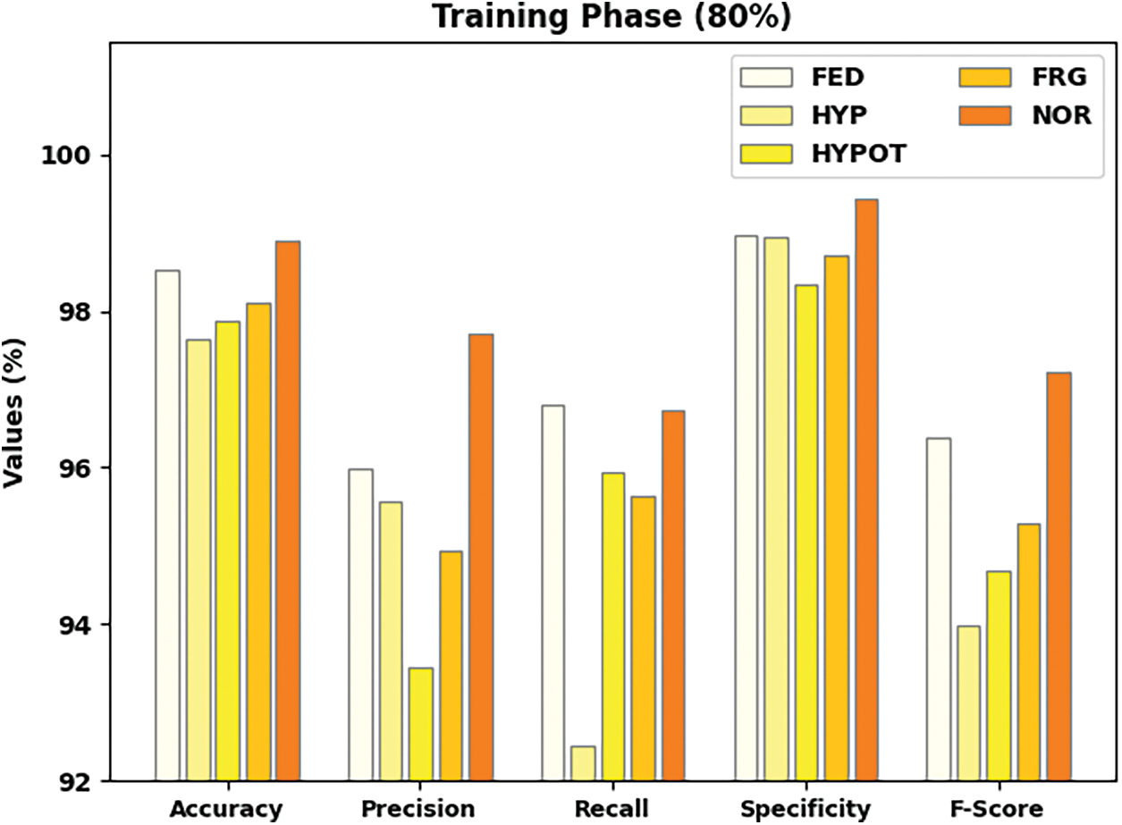
Figure 4: Result analysis of IFBC-MIWOEF method under 80% of TR data
Fig. 5 depicts the total organization consequences of the IFBC-MIWOEF technique on 20% of TS data. The figure indicates that the IFBC-MIWOEF technique has demonstrated improved outcomes under each class label. For example, the IFBC-MIWOEF method has classified samples under the FED class with
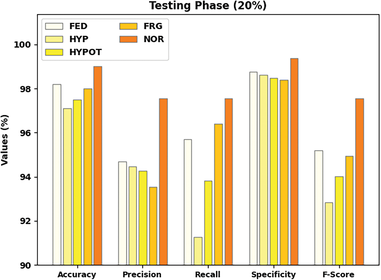
Figure 5: Result analysis of IFBC-MIWOEF method under 20% of TS data
A brief fish behavior categorization result using the IFBC-MIWOEF methodology under the 70% TR and 30% TS dataset is provided in Table 3. The overall classification results of the IFBC-MIWOEF technique are shown in Fig. 6 using data from 70% of the TR dataset. According to the figure, the IFBC-MIWOEF technique has improved results for each class label. For example, the IFBC-MIWOEF technique has classified samples under the FED class with

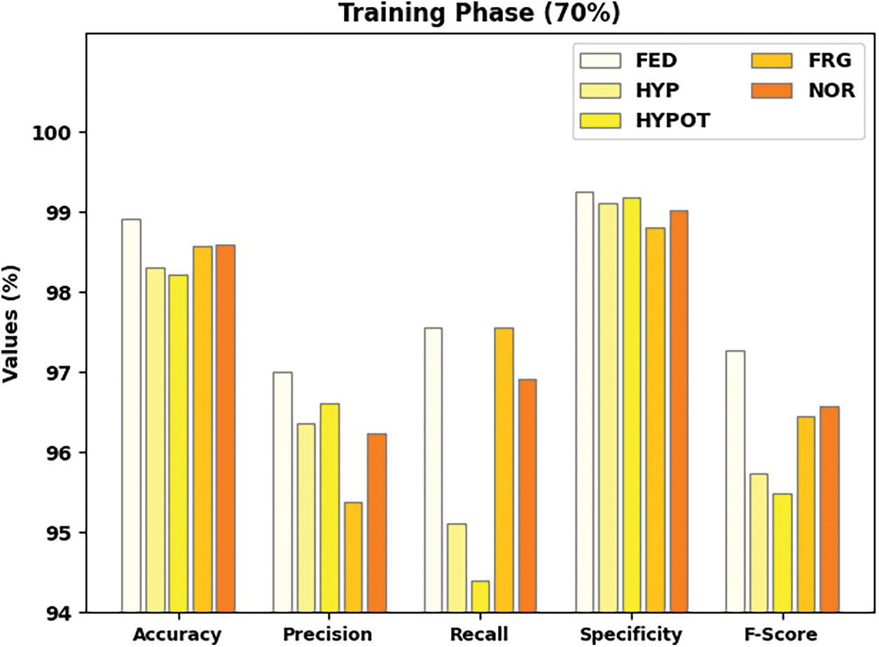
Figure 6: Result analysis of IFBC-MIWOEF method under 70% of TR data
Fig. 7 demonstrates the total organization consequences of the IFBC-MIWOEF method on 30% of the TS dataset. The figure shows that the IFBC-MIWOEF method has demonstrated improved outcomes under each class label. For example, the IFBC-MIWOEF method has classified samples under the FED class with
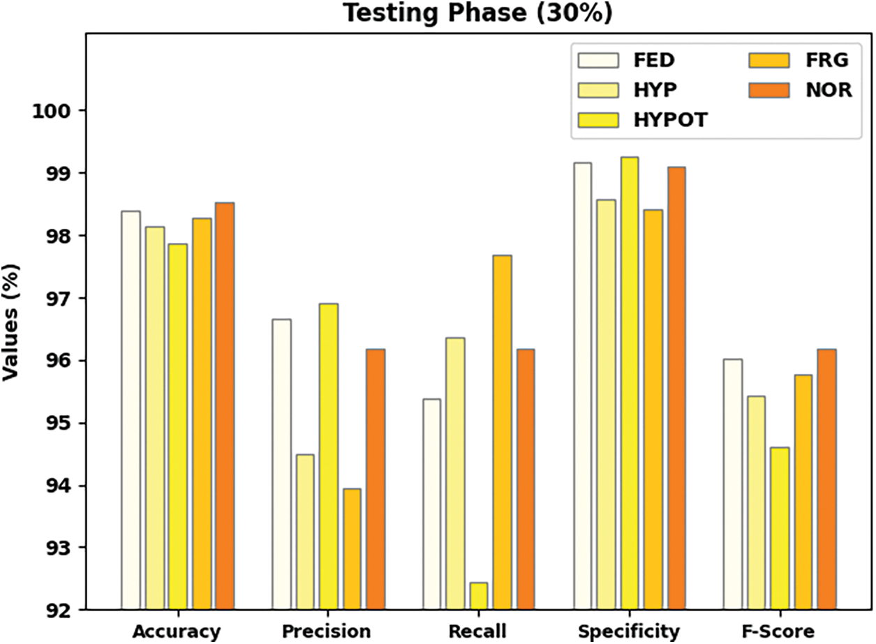
Figure 7: Result analysis of IFBC-MIWOEF method under 30% of TS data
Table 4 demonstrates the comparison study of the IFBC-MIWOEF model with other models. Fig. 8 reports a comparative review of the IFBC-MIWOEF with existing methodologies. The graph showed that the LeNet5 model performed poorly, with an

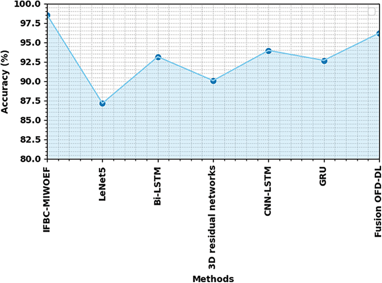
Figure 8:
The experimental results proved that the IFBC-MIWOEF model performed better than other models at recognising fish behaviour.
To identify and categorize different forms of fish behavior, a novel IFBC-MIWOEF model was developed in this study. Primarily, the input videos are collected, and the frame conversion process takes place. Then, the fusion-based feature extraction process is carried out through three DL algorithms, namely VGG-19, DenseNet, and EfficientNet. The performance of the DL models can be improvised using the MIWO algorithm-based hyperparameter tuning process. Finally, the SM layer assigns the incoming video frames appropriate class labels. To demonstrate the efficacy of the IFBC-MIWOEF model, a series of imitations were performed using distinct processes. An Extensive comparative study pointed out the better outcomes of the IFBC-MIWOEF model over current methods. Thus, the presented IFBC-MIWOEF approach can be treated as a professional fish behavior recognition and classification tool.
Funding Statement: The authors received no specific funding for this study.
Availability of Data and Materials: The data used to support the findings of this study are available from the corresponding author upon request.
Conflicts of Interest: The authors declare that they have no conflicts of interest to report regarding the present study.
References
1. S. Zhao, S. Zhang, J. Liu, H. Wang, J. Zhu et al., “Application of machine learning in intelligent fish aquaculture: A review,” Aquaculture, vol. 540, pp. 736724, 2021. [Google Scholar]
2. M. Sun, X. Yang and Y. Xie, “Deep learning in aquaculture: A review,” Journal of Computers, vol. 31, no. 1, pp. 294–319, 2020. [Google Scholar]
3. C. Xia, L. Fu, Z. Liu, H. Liu, L. Chen et al., “Aquatic toxic analysis by monitoring fish behavior using computer vision: A recent progress,” Journal of Toxicology, vol. 2018, no. 2, pp. 1–15, 2018. [Google Scholar]
4. M. Susmita and P. Mohan, “Digital mammogram inferencing system using intuitionistic fuzzy theory,” Computer Systems Science and Engineering, vol. 41, no. 3, pp. 1099–1115, 2022. [Google Scholar]
5. B. V. Deep and R. Dash, “Underwater fish species recognition using deep learning techniques,” in 6th Int. Conf. on Signal Processing and Integrated Networks (SPIN), Noida, India, pp. 665–669, 2019. [Google Scholar]
6. L. Yang, Y. Liu, H. Yu, X. Fang, L. Song et al., “Computer vision models in intelligent aquaculture with emphasis on fish detection and behavior analysis: A review,” Archives of Computational Methods in Engineering, vol. 28, no. 4, pp. 2785–2816, 2021. [Google Scholar]
7. W. Xu and S. Matzner, “Underwater fish detection using deep learning for water power applications,” in Int. Conf. on Computational Science and Computational Intelligence (CSCI), Las Vegas, NV, USA, pp. 313–318, 2018. [Google Scholar]
8. D. Li, Z. Wang, S. Wu, Z. Miao, L. Du et al., “Automatic recognition methods of fish feeding behavior in aquaculture: A review,” Aquaculture, vol. 528, pp. 735508, 2020. [Google Scholar]
9. A. Banan, A. Nasiri and A. Taheri-Garavand, “Deep learning-based appear-ance features extraction for automated carp species identification,” Aquacultural Engineering, vol. 89, pp. 102053, 2022. [Google Scholar]
10. B. Jaishankar, A. Pundir, I. Patel and N. Arulkumar, “Blockchain for securing healthcare data using squirrel search optimization algorithm,” Intelligent Automation & Soft Computing, vol. 32, no. 3, pp. 1815–1829, 2022. [Google Scholar]
11. M. A. Iqbal, Z. Wang, Z. A. Ali and S. Riaz, “Automatic fish species classification using deep convolutional neural networks,” Wireless Personal Communications, vol. 116, no. 2, pp. 1043–1053, 2021. [Google Scholar]
12. A. Jalal, A. Salman, A. Mian and F. Shafait, “Fish detection and species classification in underwater environments using deep learning with temporal information,” Ecological Informatics, vol. 57, pp. 101088, 2020. [Google Scholar]
13. A. B. Tamou, A. Benzinou, K. Nasreddine and L. Ballihi, “Underwater live fish recognition by deep learning,” in Int. Conf. on Image and Signal Processing, Cherbourg, France, Springer, pp. 275–283, 2018. [Google Scholar]
14. H. S. Chhabra, A. K. Srivastava and R. Nijhawan, “A hybrid deep learning ap-proach for automatic fish classification,” in Proc. of ICETIT 2019, Institutional Area, Janakpuri New Delhi, Springer, pp. 427–436, 2020. [Google Scholar]
15. C. Zhou, D. Xu, L. Chen, S. Zhang, C. Sun et al., “Evaluation of fish feeding intensity in aquaculture using a convolutional neural network and machine vision,” Aquaculture, vol. 507, pp. 457–465, 2019. [Google Scholar]
16. M. U. Farooq, M. N. M. Saad and S. D. Khan, “Motion-shape-based deep learning approach for divergence behavior detection in high-density crowd,” Visual Computer, vol. 38, pp. 1553–1577, 2022. [Google Scholar]
17. S. D. Khan, Y. Salih, B. Zafar and A. Noorwali, “A deep-fusion network for crowd counting in high-density crowded scenes,” International Journal Computer Intelligence System, vol. 14, pp. 168, 2021. [Google Scholar]
18. A. J. Alzahrani and S. D. Khan, “Characterization of different crowd behaviors using novel deep learning framework,” Turkish Journal of Electrical Engineering & Computer Sciences, vol. 29, pp. 169–185, 2021. [Google Scholar]
19. S. D. Khan, S. Bandini, S. Basalamah and G. Vizzari, “Analysing crowd behavior in naturalistic conditions: Identifying sources and sinks and characterizing main flows,” Neurocomputing, vol. 177, no. 5, pp. 543–563, 2016. [Google Scholar]
20. K. M. Knausgård, A. Wiklund, T. K. Sørdalen, K. T. Halvorsen, A. R. Kleiven et al., “Temperate fish detection and classification: A deep learning-based approach,” Applied Intelligence, vol. 52, no. 6, pp. 6988–7001, 2020. [Google Scholar]
21. M. Revanesh, V. Sridhar and J. M. Acken, “CB-ALCA: A cluster-based adaptive lightweight cryptographic algorithm for secure routing in wireless sensor networks,” International Journal of Information and Computer Security, vol. 11, no. 6, pp. 637–662, 2019. [Google Scholar]
22. G. Wang, A. Muhammad, C. Liu, L. Du and D. Li, “Automatic recognition of fish behavior with a fusion of RGB and optical flow data based on deep learning,” Animals, vol. 11, no. 10, pp. 2774, 2021. [Google Scholar] [PubMed]
23. M. R. Hassan, M. F. Islam, M. Z. Uddin, G. Ghoshal, M. M. Hassan et al., “Prostate cancer classification from ultrasound and MRI images using deep learning based Explainable Artificial Intelligence,” Future Generation Computer Systems, vol. 127, pp. 462–472, 2022. [Google Scholar]
24. C. Saravanakumar, R. Priscilla, B. Prabha, A. Kavitha and C. Arun, “An efficient on-demand virtual machine migration in cloud using common de-ployment model,” Computer Systems Science and Engineering, vol. 42, no. 1, pp. 245–256, 2022. [Google Scholar]
25. R. R. Bhukya, B. M. Hardas and T. Ch, “An automated word embedding with parameter tuned model for web crawling,” Intelligent Automation & Soft Computing, vol. 32, no. 3, pp. 1617–1632, 2022. [Google Scholar]
26. C. Pretty Diana Cyril, J. Rene Beulah, A. Harshavardhan and D. Sivabalaselvamani, “An automated learning model for sentiment analysis and data classification of Twitter data using balanced CA-SVM,” Concurrent Engineering: Research and Applications, vol. 29, no. 4, pp. 386–395, 2021. [Google Scholar]
27. P. V. Rajaram and P. Mohan, “Intelligent deep learning based bidirectional long short term memory model for automated reply of e-mail client prototype,” Pattern Recognition Letters, vol. 152, no. 10, pp. 340–347, 2021. [Google Scholar]
28. V. Harshavardhan and S. Velmurugan, “Chaotic salp swarm optimization-based energy-aware VMP technique for cloud data centers,” Computational Intelligence and Neuroscience, vol. 2022, no. 4, pp. 1–16, 2022. [Google Scholar]
29. J. Deepak Kumar, B. Prasanthi and J. Venkatesh, “An intelligent cognitive-inspired computing with big data analytics framework for sentiment analysis and classification,” Information Processing & Management, vol. 59, no. 1, pp. 1–15, 2022. [Google Scholar]
30. D. K. Jain, S. K. Sah Tyagi and N. Subramani, “Metaheuristic optimization-based resource allocation technique for cybertwin-driven 6G on IoE environment,” IEEE Transactions on Industrial Informatics, vol. 18, no. 7, pp. 4884–4892, 2022. [Google Scholar]
31. B. M. Hardas and S. B. Pokle, “Optimization of peak to average power reduction in OFDM,” Journal of Communications Technology and Electronics, vol. 62, pp. 1388–1395, 2017. [Google Scholar]
32. Y. Alotaibi, S. Alghamdi and O. I. Khalaf, “An efficient metaheuristic-based clustering with routing protocol for underwater wireless sensor networks,” Sensors, vol. 22, no. 2, pp. 1–15, 2022. [Google Scholar]
33. T. Satish Kumar, S. Jothilakshmi, B. C. James and N. Arulkumar, “HHO-based vector quantization technique for biomedical image compression in cloud computing,” International Journal of Image and Graphics, vol. 23, no. 3, pp. 1–15, 2022. [Google Scholar]
34. H. Y. Sang, Q. K. Pan, J. Q. Li, P. Wang and Y. Y. Han, “Effective invasive weed optimization algorithms for distributed assembly permutation flow shop problem with total flowtime criterion,” Swarm and Evolutionary Computation, vol. 44, pp. 64–73, 2019. [Google Scholar]
35. Y. Alotaibi, S. Alghamdi, O. I. Khalaf and U. Sakthi, “Improved metaheuristics-based clustering with multihop routing protocol for underwater wireless sensor networks,” Sensors, vol. 22, no. 4, pp. 1–16, 2022. [Google Scholar]
36. D. Paulraj and P. Ezhumalai, “A deep learning modified neural network (DLMNN) based proficient sentiment analysis technique on twitter data,” Journal of Experimental & Theoretical Artificial Intelligence, pp. 1–15, 2022. https://doi.org/10.1080/0952813X.2022.2093405 [Google Scholar] [CrossRef]
37. B. T. Geetha, A. K. Nanda, A. M. Metwally, M. Santhamoorthy and M. S. Gupta, “Metaheuristics with deep transfer learning enabled detection and classification model for industrial waste management,” Chemosphere, vol. 308, no. 10, pp. 1–13, 2022. [Google Scholar]
38. S. Raghavendra, B. T. Geetha, S. M. R. Asha and M. K. Roberts, “Artificial humming bird with data science enabled stability prediction model for smart grids,” Sustainable Computing: Informatics and Systems, vol. 36, no. 9, pp. 1–17, 2022. [Google Scholar]
39. D. K. Jain and X. Liu, “Modeling of human action recognition using hyperparameter tuned deep learning model,” Journal of Electronic Imaging, vol. 32, no. 1, pp. 1–10, 2022. [Google Scholar]
40. E. Veerappampalayam, N. Subramani, M. Subramanian and S. Meckanzi, “Handcrafted deep-feature-based brain tumor detection and classification using MRI images,” Electronics, vol. 11, no. 24, pp. 1–10, 2022. [Google Scholar]
41. A. Mardani, A. R. Mishra and P. Ezhumalai, “A fuzzy logic and DEEC protocol-based clustering routing method for wireless sensor networks,” AIMS Mathematics, vol. 8, no. 4, pp. 8310–8331, 2023. [Google Scholar]
42. V. D. Ambeth Kumar, S. Malathi, K. Abhishek Kumar and K. C. Veluvolu, “Active volume control in smart phones based on user activity and ambient noise,” Sensors, vol. 20, no. 15, pp. 1–15, 2020. [Google Scholar]
43. C. Ramalingam, “An efficient applications cloud interoperability framework using I-Anfis,” Symmetry, vol. 13, no. 2, pp. 1–15, 2021. [Google Scholar]
44. R. Chithambaramani, “Addressing semantics standards for cloud portability and interoperability in multi cloud environment,” Symmetry, vol. 13, no. 2, pp. 1–14, 2021. [Google Scholar]
Cite This Article
 Copyright © 2023 The Author(s). Published by Tech Science Press.
This work is licensed under a Creative Commons Attribution 4.0 International License , which permits unrestricted use, distribution, and reproduction in any medium, provided the original work is properly cited.
 Downloads
 Citation Tools