Detection of a Quasiperiodic Phenomenon of a Binary Star System Using Convolutional Neural Network

1  Introduction

A signal is a phenomenon, an event, or a function that transmits encoded information. It can take on various shapes, including electromagnetic waves, energy, impulse, optical, mechanical, acoustic, and many more [1]. It is conveyed between the receiver and the transmitter, both of which may be fundamentally opposed in how they are created, received, and processed [2].

Astrophysical signals are documented as electromagnetic radiation by either device on the ground that can monitor a range of low to medium frequencies (GHz to THz, optical region) or satellite systems in Earth’s orbit because of cosmic radiation filtering and the atmosphere. The latter manifest in THz and higher frequency spectra (ultraviolet, gamma, beta radiation, etc.) [3]. In the current years, astronomical satellites are undergoing rapid development and are collecting vast amounts of data daily. The quantity of data generated by these satellites is immense, leading to the construction of large-scale data archives. For instance, the HEASARC astrophysical scientific archive is presently archiving data from 20 satellites over a period of 30 years, specifically high-frequency data. In our research, we investigate satellite-observed low-frequency and low-energy signals [4].

Our focus will be on analyzing the data from the Kepler satellite, which observed a binary star system named MV Lyrae, belonging to the category of CVs. The CVs comprise a primary star that draws in material from its host, which is a secondary star. Within the CVs, there are numerous phenomena that can be examined. In our study, we will be exploring a particular phenomenon that exhibits stochastic behavior rather than following a specific occurrence period. This phenomenon is known as the quasiperiodic oscillations (QPOs) of the accreted mass which then forms an accretion disc around the host star. Our observed CV is a binary star system called MV Lyrae [4]. The nature of QPOs is defined by a continuous range of frequencies that are not harmonically associated with one another. In other words, a QPOs frequency fluctuates with time, but the pattern of fluctuation repeats across larger time scales. On the other hand, there are so-called pseudo-periodic oscillations (PPOs), defined by a non-repeating pattern of oscillation that seems to be periodic across a restricted spectrum of time scales. Unlike QPOs, the frequency of a PPO does not fluctuate continuously but rather jumps between discrete values. PPOs are frequently seen in chaotic systems, such as the behavior of a pendulum in the presence of random force [5–7].

CVs have demonstrated the presence of QPOs across a range of time scales. Some CVs have exhibited rapid QPOs with a period of a few milliseconds. The QPOs are thought to originate from the shock zone between a white dwarf and accretion streams [8]. X-ray astronomy employs the term QPO to describe the fluctuations in X-ray light emanating from astronomical objects at specific frequencies. These oscillations occur when X-rays are emitted in the vicinity of the inner edge of an accretion disk where gas is spiraling onto a compact object, such as a white dwarf, neutron star, or black hole [9]. The study of QPOs holds significant potential for astronomers in terms of gaining insight into the innermost areas of the accretion discs, as well as the masses, radii, and spin periods of not only white dwarfs but also neutron stars and black holes. Furthermore, QPOs have the potential to provide insights that could help test Albert Einstein’s theory of general relativity. This theory predicts outcomes that differ from those predicted by Newtonian gravity when the gravitational force is at its strongest or when there is rapid rotation [10].

To analyze our QPO signals, various software tools are currently utilized, as manual processing of this signal can be a difficult task for scientists. The potential for artificial intelligence (AI) techniques to aid in this process is significant, as it could reduce the time and effort required for signal analysis and estimation. ML is a particularly useful tool for analyzing large volumes of data and is becoming increasingly utilized in various applications such as medicine (for identifying tumors), weather forecasting, stock price forecasting, voice recognition, and object generation. The input into such a system can be in the form of an image, numerical matrix, or text string, and depending on the specific problem, an ML algorithm can learn to recognize certain patterns or characteristics and generate or predict new outputs accordingly. Python will be the language we utilize for programming due to the numerous functions and data analysis tools available without licensing fees in its libraries. Python is a common choice for scientists and offers intricate data analysis capabilities. The rest of the paper is organized as follows. Section 2 brings more insight into the data we work with as well as its preparation. Section 3 contains the basic terminology and methodology used in this work. Section 4 contains the results. Section 5 contains the discussion. Section 6 contains the conclusions and policy implications. In the end, the references used are listed.

2  Signal Processing, Timing Analysis

Our research specifically focuses on the study of a binary star system called MV Lyrae, which is a CV. Although it may not be apparent, such star systems are prevalent in the universe. Our investigation centers on analyzing the photometric signal obtained from the Kepler space telescope. The spacecraft was equipped with charge-coupled device (CCD) cameras that function by capturing photons in the field of view through a network of 42 photometers. The CCD chip detects these as an electric charge and records them over time [11–13]. The observational data were archived in the Mikulski Archive for Space Telescopes (MAST). Before our analysis of the data, the raw CCD data must be processed using proper software such as SaS, Heasoft, or Fits View. We used the Fits View software. The energy of the photons and the time of its recording are used to create a critical product for our timing analysis research called a light curve. The light curve, we were working with, is presented in Fig. 1. Expert astronomers can detect some variations in the light curve, but the pattern of its occurrence is not consistent.

Figure 1: The 272-day-long light curve of our research object, a CV called MV Lyrae

Our initial step is to process the signal by removing gaps and zeros from the data to obtain a continuous curve. Afterward, we continue the process by dividing the 272-day-long light curve into equal 1-day-long parts. The flux of each target day was then evaluated using the Lomb-Scargle [14] procedure to figure out the signal’s strength in each time. We get the next product required for our analysis called a periodogram. We grouped every 10 periodograms together (see Fig. 2) and used a log-log scale, to get a better understanding of our data. As we can see, there is a steep decline in the power of the signal to higher frequencies beginning at log(f/Hz) ≃ −3, meaning the presence of QPOs as mentioned in reference [11]. To obtain a PDS, we utilized Bartlett’s method [15] to average the 10-day periodogram. Each bin in the PDS represents the signal’s power at a specific frequency, along with a standard deviation calculated from the 10 averaged values used.

Figure 2: Grouped Lomb-Scargle [14] periodograms of MV Lyrae, ranging from day 401–411. The light curve from which the periodogram was created is in the inset figure

The resulting PDS bins (Fig. 3, black bars) show slope profiles, those are the manifesting QPOs. Some QPOs are obvious, such as the one at log(f/Hz) ≃ −2.9, while others are more subtle. Our attention is drawn to the QPO at log(f/Hz) ≃ −3.4. This QPO is exceedingly weak, appearing only in three bins of the PDS. Scientists already hypothesized that most binary star systems exhibit a similarly subtle QPO at the frequency mentioned earlier [16–18]. To accurately describe our data, we need to identify a model that fits our observations. Lorentz models are commonly used to describe QPO peaks [19], so we used a three (to simulate data without the QPO) and a four (for the simulation of data with the researched QPO) Lorentz component models to create representative fits of our data.

Figure 3: Constructed PDS bins (black bars) with 1-sigma confidence interval (blue dashed line) and fitted four component Lorentz model (red solid line)

In Eq. (1), a single Lorentz model is defined with a constant K describing the y-axis offset, an amplitude A of the Lorentz profile, a centroid c, and the width of the Lorentz profile w. A Lorentz model can be created by summing the single Lorentz profiles with different parameters to describe the QPOs.

L=K+(A⋅w(x−c)2+w2)(1)

To estimate the confidence of our QPO, we generated Timmer & Koenig simulations [20]. The input to each simulation is the fitted parameters from the Lorentz model. Each simulation produces a synthetic light curve, which needs to be processed the same way as we did with our real observational data, i.e., using Lomb-Scargle [14] and afterward Bartlett’s method [15] to produce a PDS either with or without the QPO of our interest (based off the parameters of the fit describing our real data). Afterward, we calculated the sigma confidence intervals. Our observed frequency (the three bins near log(f/Hz) ≃ −3.4) fell below the 1 − σ interval, indicating a confidence level below 68%. This is not significant enough to be considered conclusive.

To improve the confidence level of identifying our QPO, we plan to implement an ML method using simulated light curves and PDS images. For training purposes, we will divide the images into two categories called 4lor (consisting of simulated light curves and the respective PDS with the QPO at our frequency of interest) and 3lor (light curves and the PDS without it). The PDS and light curves will be used in the selected ML algorithms as image input. We will train the ML algorithms using datasets of various sizes, ranging from 50 to 5000 samples from each category.

3  Machine Learning Methods

ML is a subset of AI that involves training algorithms able to learn patterns in data, without being explicitly programmed. It is a process of training a model on a dataset to learn the relationships between inputs and outputs, and then using that model to make predictions or classify new data [21]. There are three main types of ML: supervised learning, unsupervised learning, and reinforcement learning [22]. In supervised learning, the model is trained on labeled data, where the desired output is known for each input. In unsupervised learning, the model is trained on unlabeled data, and it must find patterns or structures in the data without any prior knowledge of the output. In reinforcement learning, the model learns by interacting with an environment and receiving rewards or punishments for its actions [23,24]. ML has a wide range of practical applications, including image and speech recognition, natural language processing, recommendation systems, fraud detection, and more. It has been used in industries such as healthcare, finance, and transportation to make predictions and optimize processes [25].

In ML, a loss function is used to measure the difference between predicted and actual values. It is a mathematical function (2) that takes input from the model’s prediction and the true target values and outputs a scalar value that represents the cost incurred by the model for the prediction. The goal of training an ML model is to minimize the loss function. A commonly used loss function is the mean squared error (MSE) given by:

MSE=1n∑(y−y_pred)2(2)

where y and y_pred are the true and predicted values, respectively, and n is the number of samples in the training dataset. In classification problems, cross-entropy loss is often used [22,26].

Artificial neural networks (ANNs) are a class of ML models inspired by the structure and function of biological neurons. ANNs consist of multiple interconnected nodes (neurons) that process information and learn to make predictions based on input data. Convolutional neural networks (CNNs) are a type of ANNs that are commonly used in image and video processing tasks. They use convolutional layers to automatically learn features from raw pixel data. Sequential models are a type of ANN used in sequential data processing tasks, such as natural language processing and time series prediction. These models learn to predict the next value in a sequence based on previous values [22,25,27].

While in our previous research, as in reference [28], we worked with numerical data, the results were not as we expected, with a QPO detection accuracy of roughly 60% while using a support vector machine and a recurrent neural network. Based on our results, we were certain, that we need to use less procession of the raw data i.e., the usage of light curves rather than PDS, especially when working with numerical data. In this work, we will work with CNN models which are commonly used for image data. We will use our simulated light curves in the form of an image as the training dataset. As we mentioned, we will have two categories, with and without the QPO based on the fit used. Optimization algorithms play a crucial role in training CNNs to achieve high performance in computer vision tasks. The most widely used optimization algorithm for training CNNs is stochastic gradient descent (SGD), which updates the network parameters based on the gradients of the loss function with respect to the parameters. Other optimization algorithms, such as Adam, Adagrad, and RMSProp, have also been developed to improve the convergence speed and stability of the training process. Additionally, techniques such as weight decay, dropout, and batch normalization are commonly used to regularize the network and prevent overfitting [29,30]. The choice of optimization algorithm and regularization techniques can significantly impact the network’s performance. Researchers continue to explore new optimization algorithms and techniques to further improve the training of CNNs. As the area of ML is growing, so is its usage in various scientific fields. Astronomy can also benefit from ML model utilization. The following works demonstrate the versatility of CNNs in astronomy, including applications such as galaxy morphology prediction, photometric redshift estimation, and object detection in astronomical images. Additionally, recent studies have explored the use of deep learning for cosmological parameter estimation, showing promising results in overcoming the effects of galaxy morphology on parameter inference. Sadly, we did not find any relevant works regarding the detection of QPO using CNNs.

Authors in reference [31] developed a convolutional neural network (CNN) for the detection of transiting exoplanets in time-domain data. The CNN was trained on simulated data and then applied to real-world observations from the K2 mission. The CNN achieved a high detection accuracy and was able to identify previously undiscovered exoplanets, demonstrating the effectiveness of CNNs in analyzing time series data from astronomical observations. Their accuracy of detection was 88.5%.

In reference [32], the authors investigated the use of diverse convolutional neural networks for time series classification. The authors proposed a novel architecture that combined multiple CNNs with different kernel sizes and pooling strategies. The proposed model was evaluated on several benchmark datasets and demonstrated state-of-the-art performance compared to other methods. Although their detection accuracy was roughly 74%, the study highlights the potential of using diverse CNNs to improve the accuracy of time series classification tasks. explored the use of deep learning techniques, specifically CNNs, for predicting the morphologies of galaxies.

The authors in reference [33] trained a CNN on a large dataset of labeled galaxy images from the Galaxy Zoo project and achieved an accuracy of 92% in predicting galaxy morphology types. They also compared the performance of their CNN with that of other ML algorithms and found that the CNN outperformed these methods in terms of accuracy and computational efficiency. presented a deep-learning approach for classifying galaxy morphology.

The researchers of the paper in the reference [34] used a CNN to analyze and classify galaxy images from the K-CLASH (Kilo-Degree Cluster Lensing and Supernova Survey with Hubble) dataset. The near-perfect results of 99 % accuracy showed that the CNN was able to accurately classify the majority of the galaxies according to their morphology, including distinguishing between elliptical and spiral galaxies. This approach can be used to significantly speed up the analysis of large datasets in astronomy, where manual classification of galaxy morphology can be very time-consuming.

The authors in reference [35] proposed a CNN to analyze X-ray data from the Chandra and XMM-Newton telescopes. The results showed that the CNN was able to estimate the X-ray mass and gas fraction of the galaxy clusters with a precision comparable to traditional methods but significantly faster.

FETCH (Fast Extragalactic Transient Candidate Hunter) [36] is a deep learning-based classifier designed for rapid and accurate classification of fast transients in astronomical data. The model uses convolutional neural networks to identify and classify transients based on their light curves, or time series of brightness measurements. The authors trained FETCH on a large set of simulated and real data, achieving high accuracy (99.5%) and fast classification times.

The authors in reference [37] used supervised ML algorithms to classify fast radio bursts (FRBs) detected by the CHIME telescope. The researchers applied several different ML techniques to the data, including support vector machines, random forests, and artificial neural networks. The results showed that the ML algorithms could accurately classify the FRBs based on their observed properties, such as their dispersion measure and signal-to-noise ratio. The study also identified several new FRB candidates that were missed by traditional detection methods, demonstrating the potential of ML for discovering new phenomena in the universe.

In the paper by [38], they applied deep learning techniques to detect and classify gravitational waves from neutron star-black hole mergers. The researchers trained a deep neural network on simulated gravitational wave data and found that it was able to accurately (with about 90% certainty) detect and classify these events with high precision. The study suggests that deep learning methods can significantly improve the detection and analysis of gravitational waves, opening new avenues for studying the universe and testing fundamental physics.

The study by [39] used ML algorithms to identify active galactic nuclei (AGNs) from the HETDEX survey data. The researchers applied a random forest classifier to a large sample of galaxies and found that it was able to accurately identify AGNs based on their spectral properties. The study also compared the performance of different ML algorithms and found that random forest performed better than other techniques. The results (accuracy of about 92%) show that ML can be a powerful tool for identifying and studying AGNs in large surveys, providing insights into the evolution of galaxies and the supermassive black holes that power these phenomena.

The examples mentioned demonstrate the effectiveness of ML algorithms beyond image-based detection. Based on the literature review, we have a hypothesis that a CNN will detect our subtle QPO while trained on the very images of the light curves. We also compared the CNN to other state-of-the-art algorithms such as a random forest, a recurrent network, and an artificial neural network. Our research objective is to utilize a CNN to address the issue of detecting faint QPO signals and evaluate our findings in comparison to the conventional method of estimating confidence, namely Timmer & Koenig’s confidence intervals [20]. The total research flowchart is presented in Fig. 4.

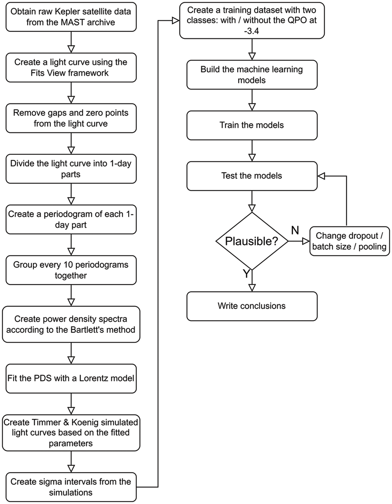
Figure 4: Flowchart of our research

We have decided to use light curves, in the form of an image, to create a training dataset for our CNN. The ML model was created using the Keras 2.10 library of Python 3.9.16. First, we simulated 50–5000 samples of light curve images in each category, e.g., with the QPO of our interest (using a fit with three Lorentz components) and without the QPO at the researched frequency. Afterward, we divided the data into training (80% of the whole dataset) and validation (20% of the dataset) sets.

We used rescaling of each image so that the numerical matrix passed to the CNN has values in between 1–255 to represent a numerical RGB spectrum. We also used data augmentation of the train set. Here we rotated the image by 20% and zoomed in by 20% of their original position as well as set the image size for the input layer of our model to 180 × 180 pixels. To build the model, we used the Sequential function of the Keras library, and the resulting model is depicted in Fig. 5.

Figure 5: Architecture of our CNN model

The first layer is the input layer, where data augmentation and rescaling are utilized. Next are 2D convolutions with added pooling layers. We tested several combinations of numbers of neurons and convolution layers in the range of 2–128 and the best-performing combination was two convolution layers with 32 neurons, with a pooling layer after each, and a convolution layer with 64 neurons, also with a pooling layer afterward. The rest of the model consists of a dropout layer with a 60% dropout, one layer to flatten the output tensor of the convolutional layer for a fully connected (dense) layer, which is the last layer and has two neurons based on the number of our classes. For the optimization algorithm of our model, Adam was used. We also tested other algorithms, i.e., adaptive momentum with gradient descent, root mean square propagation, and stochastic gradient descent, but those were not performing well and often got stuck in local minima, resulting in an unsuccessful training of the model. To obtain the best training results, we also utilized an early stopping callback, so the model does not overfit. Here we monitored the validation accuracy with a patience of 50 epochs and if the improvement in the accuracy is less than 0.01, the training stops. The initial number of epochs was 300. We used several dataset sizes ranging from 50 to 5000 to see if the results will change. An increasing value of batch size proved to be beneficial for each dataset size. The training and validation accuracy and loss curves are shown in Fig. 6. Each row of the figure represents each training dataset size, i.e., a1, a2 depict metrics for the model trained on dataset size of 50, b1, b2 are metrics for a model trained on 100 samples, etc. The best training and validation results were while using the 5000-size training dataset. The metrics of the CNNs training are also summarized in Table 1.

Figure 6: Training and testing metrics for our CNN models. Displayed are training accuracy (black line), validation accuracy (blue line), training loss (red line), and validation loss (green line)

Based on the results, we can see that the training accuracy accurately matches the validation accuracy in most of the cases, meaning the process of training our CNN models was successful. The best validation accuracy yielded a model trained on 5000 samples of each category. And as we will see, the best testing results will also yield this CNN model.

4  Results

We tested each model with 10000 simulated data (with the QPO at log(f/Hz) ≃ −3.4), different from the training data. We employed a statistic so that we will monitor how many samples will be classified with a prediction accuracy of less than 68% (meaning falling under the 1 − σ interval in Timmer & Koenig’s confidence levels [20]), how many samples will have prediction accuracy between 68% and 95% (1 − σ), how many will fall between 95% and 99.7% (2 − σ) and above 99.7% (3 − σ). The performance of each CNN model is summarized in Table 2.

We can clearly see, that increasing the dataset size helped the CNN to extract more necessary features. Each trained model had different training batch sizes, i.e., 1, 2, 5, 10, 20, 50. We chose the batch size as approximately 10% of the training dataset size. The most well-performing size of training data was 5000 (from each category), with a batch size of 50. The results of testing this CNN are as follows: out of the 10000-testing data, 2171 were in the 68%–95% interval of confidence, 2437 had classification accuracy between 95%–99.7%, and 4652 had classification accuracy above 99.7%. We can say that 71% of the whole testing dataset was classified above 95% as 4lor, giving us confidence of 2 − σ and above. This proves our hypothesis, that using light curves in an image format, rather than numerical training data, will yield better results. We were also surprised, that our CNN was able to extract the necessary features to find QPO even in noisy data. This only proves the robustness of the CNNs. The worst performing was, as anticipated, the model trained using 50 samples of each class and a batch size of 1.

The best-in-case classification CNN model did outperform the Timmer & Koenig [20] method of estimating confidence. We created PDS out of the light curves tested because we could not tell from a light curve, where (or if) there are any QPO present. Fig. 7 shows 4 simulated PDS constructed from the testing light curves, which were classified above 99.7% as 4lor using our trained CNN model, giving it confidence of 3 − sσ. We created Timmer & Koenig confidence intervals [20] to see, where the QPO at log(f/Hz) ≃ −3.4 will fall.

Figure 7: Simulated light curves (first column) classified as 4lor with over 99.7% confidence. A 4-component Lorentz profile (second column, red line) was fitted, and the Timmer & Koenig confidence intervals [20] (second column, blue dashed line) were generated alongside the PDS (second column, black bars)

In Fig. 7, the target QPO’s confidence levels estimated using Timmer & Koenig [20] were below the 1 − σ giving the QPO confidence of under 68%, while our CNN classified the QPO with 99.7% confidence as 4lor (the category with the QPO present) This proves, we were successful in both training our CNN model and creating a better confidence tool for estimating the confidence of QPOs at log(f/Hz) ≃ −3.4 just from a light curve image. To clarify, the researched QPO frequency in the top right panel of Fig. 7 is log(f/Hz) ≃ −3.40 while the bottom right panel demonstrated a frequency of log(f/Hz) ≃ −3.43. In a longer timescale, such as when analyzing our 272-day-long light curve, we saw a pattern. On every 10th day, a QPO manifested with a frequency of log(f/Hz) ≃ −3.40, while a QPO with a frequency of log(f/Hz) ≃ −3.38 manifested every 12th day. This proves that the oscillations are indeed quasiperiodic.

We also tested the viability of other algorithms e.g., artificial network, recurrent network, and a random forest. We searched for optimal parameters and those are depicted in Table 3. The testing metrics are summarized in Table 4.

For the random forest classifier, the optimal hyperparameters were as follows: the number of trees in the forest 80, the maximum depth of each decision tree 100, criterion (the function used to measure the quality of the split) mean square error, minimum numbers of samples required to split an internal branch of the tree 5. The Artificial neural network used the following hyperparameters: number of neurons in the hidden layer 20, learning rate 0.003, decay of learning rate 1e-6, batch size 10, 300 epochs with early stopping, and an Adam optimizer. The recurrent neural network used the following optimal hyperparameters: two hidden layers with tanh activation function, a learning rate of 0.001, 30 neurons in each hidden layer, a 50% dropout rate, a batch size of 15, and the Adam optimizer.

We tested each of the three algorithms using 10000 simulated data of the category 4lor, meaning that the researched QPO was present. The worst performing was the recurrent neural network with an average of 60% training and 53% testing accuracy, the metrics for the best of the three algorithms, the random forest classifier, are as follows: average training accuracy of 86% and testing accuracy 81%. Our CNN in contrast to the three algorithms got an average training accuracy of 92% and testing accuracy of 92%. This proves the supremacy of the CNN as our chosen algorithm for our task of QPO identification.

5  Discussion

To prevent common problems during the training of our CNN, we employed several countermeasures. To prevent the overfitting of our model, we used early stopping as well as a dropout.

D=α(Wx)×M(3)

In Eq. (3), W are the weights of the layer where dropout is used, x is the vector with the input data, α is the activation function (of the hidden layer in our case) and M is the binary mask that nullifies the contribution of some neurons towards the next layer [26]. The mask is generated randomly during the training process and is different for each iteration. To reduce the dimensionality of the feature maps and help to prevent the overfitting of our model, we have used pooling layers after each convolutional layer. The layer is defined as:

Mp=max(x[stride_h+p∗stride_w+q])(4)

The mathematical formulation of a pooling layer in CNNs (4) involves sliding a two-dimensional filter over each channel of the feature map and summarizing the features within the region covered by the filter [25]. In Eq. (4), Mp is the output tensor, x is the input tensor, stride_h, and stride_w are the stride values in the horizontal and vertical directions, respectively, and p and q are the pooling window’s height and width. The stride specifies the number of pixels to slide the filter at a time. When there is a limitation in training data, the model may be unable to learn all the patterns in the data, resulting in poor performance. To create surplus training data, one way is to employ data augmentation techniques such as rotating, flipping, or scaling the image data. This was especially useful and used for the smaller sizes of our training datasets. We trained a similar CNN model, but instead of light curve images, we used the images of simulated PDS created from the latter as a training set. We also trained the model using different sizes of such dataset (50–5000) and with the same sizes of training batches. The network architecture was the same as with the main model trained on light curve images. We also used the Adam optimizer, normalized the data, and employed early stopping. The resulting classification accuracies were worse than with our CNN model trained on light curves. We tested our model on 10000 simulated PDS, see Table 5.

The CNN model trained using PDS images performs in a similar way for our first three sizes of the training dataset. However, increasing the number of training images did not help to obtain better classification results. The CNN model trained with 5000 samples of each category did outperform the Timmer & Koenig method of estimating confidence intervals [20] but got worse results than our model trained using the light curves. We did not expect this result. For humans, it is easier to distinguish the QPO in a PDS, but it is clearly harder for an ML algorithm.

6  Conclusion

We analyzed the original light curve data collected from MAST of the binary star system MV Lyrae. Our time-series data analysis verifies the presence of numerous QPOs, with the anticipated QPO occurring at a frequency of log(f/Hz) ≃ −3.4. We estimated sigma confidence intervals. The researched QPO falls within the 1 − σ range using Timmer and Koenig’s method of QPO confidence estimation [20], yielding confidence of 68%. Our goal was to improve this score by implementing a CNN model that can detect such QPOs more precisely. We used simulated data, based on the parameters of the Lorentz model fitted to our PDS, to train our models. The simulated data were separated into two groups: those with and those without the target QPO present.

We conducted tests using simulated data. We also used three more algorithms to prove the supremacy of our CNN architecture. The final classification accuracy was very high. The validation accuracy of the best-in-case CNN model was 99.41% and the training accuracy was 98.60%. We tested our model with 10000 simulated light curves with the latter QPO present. Out of those, 2171 light curves were classified in the range 68%–95%, 2437 were classified in the range 95%–99.7%, and 4652 were classified above 99.7% in the category with the QPO (4lor). After additional research, we selected a few testing light curves and created a PDS out of them (Fig. 7), to show that their confidence using a common statistical method yields only confidence of under 68%. We can clearly say that using a CNN trained on synthetic light curves yields better results in classifying the QPO of our interest. This method also works for any CV object, not only MV Lyrae, manifesting a QPO at log(f/Hz) ≃ −3.4.

Funding Statement: The authors received no specific funding for this study.

Conflicts of Interest: The authors declare that they have no conflicts of interest to report regarding the present study.

References

1. A. V. Oppenheim, A. S. Willsky and S. H. Nawab, “Signals & systems,” in Prentice-Hall Signal Processing Series, 2nd ed., Upper Saddle River, N.J: Prentice Hall, 1997. [Google Scholar]

2. J. G. Proakis and D. G. Manolakis, Digital Signal Processing, 4th ed., Upper Saddle River, N.J: Pearson Prentice Hall, 2007. [Google Scholar]

3. D. E. Osterbrock and G. J. Ferland, Astrophysics of Gaseous Nebulae and Active Galactic Nuclei, 2nd ed., Sausalito, Calif: University Science Books, 2006. [Google Scholar]

4. P. Léna, D. Rouan, F. Lebrun, F. Mignard and D. Pelat, Observational Astrophysics, 3rd ed., Heidelberg: Springer, 2012. [Google Scholar]

5. S. E. Motta, “Quasiperiodic oscillations in black hole binaries,” Astronomische Nachrichten, vol. 337, no. 4–5, pp. 398–403, 2016. [Google Scholar]

6. J. P. Lasota, “Physics of accretion flows around compact objects,” Comptes Rendus Physique, vol. 8, no. 1, pp. 45–56, 2007. [Google Scholar]

7. S. H. Strogatz, Nonlinear Dynamics and Chaos: With Applications to Physics, Biology, Chemistry, and Engineering, 1st ed., Boca Raton: CRC Press, 2000. [Google Scholar]

8. B. Warner, Cataclysmic Variable Stars, 1st ed., Cambridge: Cambridge University Press, 2003. [Google Scholar]

9. A. Bianchini, M. Della Valle and M. Orio, “Cataclysmic variables,” in Proc. of Astrophysics and Space Science, Dordrecht, Netherlands, Boston, Kluwer Academic Publishers, 1995. [Google Scholar]

10. M. Livio and G. Shaviv, “Cataclysmic variables and related objects,” in Proc. of 72nd Colloquium of the Int. Astronomical Union, Haifa, Israel, Dordrecht, Springer Netherlands, vol. 101, 1983. [Google Scholar]

11. M. F. Bode and A. Evans, Classical Novae, 2nd edition, Cambridge University Press, 2008. [Google Scholar]

12. S. N. Shore, The Tapestry of Modern Astrophysics. Hoboken, N.J: Wiley-Interscience, 2011. [Google Scholar]

13. G. W. Collins, The Fundamentals of Stellar Astrophysics. New York: W.H. Freeman, 1989. [Google Scholar]

14. N. Lomb, “Least-squares frequency analysis of unequally spaced data,” Astrophysics and Space Science, vol. 39, no. 1, pp. 447–462, 1976. [Google Scholar]

15. M. S. Bartlett, “On the theoretical specification and sampling properties of autocorrelated time-series,” Supplement to the Journal of the Royal Statistical Society, vol. 8, no. 1, pp. 27–41, 1946. [Google Scholar]

16. A. Dobrotka, M. Orio, D. Benka and A. Vanderburg, “Searching for the 1 mHz variability in the flickering of V4743 Sgr: A cataclysmic variable accreting at a high rate,” Astronomy & Astrophysics, vol. 649, no. A67, pp. 1–5, 2021. [Google Scholar]

17. M. Orio, A. Dobrotka, C. Pinto, M. Henze, J. U. Ness et al., “Nova LMC 2009a as observed with XMM–Newton, compared with other novae,” Monthly Notices of the Royal Astronomical Society, vol. 505, no. 3, pp. 3113–3134, 2021. [Google Scholar]

18. A. Dobrotka, J. U. Ness and I. Bajčičáková, “Fast stochastic variability study of two SU UMa systems V1504 Cyg and V344 Lyr observed by Kepler satellite,” Monthly Notices of the Royal Astronomical Society, vol. 460, no. 1, pp. 458–466, 2016. [Google Scholar]

19. N. Bellomo and L. Preziosi, “Modelling mathematical methods and scientific computation,” in CRC Mathematical Modelling Series, vol. 32. Boca Raton: CRC Press, pp. 413–452, 1995. [Google Scholar]

20. J. Timmer and M. Koenig, “On generating power law noise,” Astronomy & Astrophysics, vol. 300, no. 1, pp. 707–710, 1995. [Google Scholar]

21. E. Alpaydin, “Introduction to Machine Learning,” in Adaptive Computation and Machine Learning, 2nd ed., Cambridge, Mass: MIT Press, 2010. [Google Scholar]

22. I. Goodfellow, Y. Bengio and A. Courville, “Deep learning,” in Adaptive Computation and Machine Learning. Cambridge, Massachusetts: The MIT Press, 2016. [Google Scholar]

23. T. Hastie, R. Tibshirani and J. Friedman, “The elements of statistical learning,” in Springer Series in Statistics. New York, NY: Springer, 2009. [Google Scholar]

24. M. I. Jordan and T. M. Mitchell, “Machine learning: Trends, perspectives, and prospects,” Science, vol. 349, no. 6245, pp. 255–260, 2015. [Google Scholar] [PubMed]

25. Y. LeCun, Y. Bengio and G. Hinton, “Deep learning,” Nature, vol. 521, no. 7553, pp. 436–444, 2015. [Google Scholar] [PubMed]

26. C. M. Bishop, “Pattern recognition and machine learning,” in Information Science and Statistics. New York, NY: Springer, 2006. [Google Scholar]

27. F. Chollet, Deep Learning with Python. Shelter Island, New York: Manning Publications Co., 2018. [Google Scholar]

28. D. Benka, S. Vašová, M. Kebísek and M. Strémy, “Detection of variable astrophysical signal using selected machine learning methods,” in Artificial Intelligence Application in Networks and Systems-Proc. of 12th Computer Science On-Line Conf., Vsetin, Czech Republic, vol. 3, 2023. [Google Scholar]

29. A. Krizhevsky, I. Sutskever and G. E. Hinton, “ImageNet classification with deep convolutional neural networks,” Communications of the ACM, vol. 60, no. 6, pp. 84–90, 2017. [Google Scholar]

30. S. Ruder, “An overview of gradient descent optimization algorithms,” 2016. https://doi.org/10.48550/ARXIV.1609.04747 [Google Scholar] [CrossRef]

31. A. Chaushev, L. Raynard, M. R. Goad, P. Eigmüller, D. J. Armstrong et al., “Classifying exoplanet candidates with convolutional neural networks: Application to the next generation transit survey,” Monthly Notices of the Royal Astronomical Society, vol. 488, no. 4, pp. 5232–5250, 2019. [Google Scholar]

32. S. Wang, S. Zhang, T. Wu, Y. Duan, L. Zhou et al., “FMDBN: A first-order Markov dynamic Bayesian network classifier with continuous attributes,” Knowledge-Based Systems, vol. 195, no. 1, pp. 1–11, 2020. [Google Scholar]

33. H. Domínguez Sánchez, M. Huertas-Company, M. Bernardi, D. Tuccillo and J. L. Fischer, “Improving galaxy morphologies for SDSS with deep learning,” Monthly Notices of the Royal Astronomical Society, vol. 476, no. 3, pp. 3661–3676, 2018. [Google Scholar]

34. J. M. Dai and J. Tong, “Galaxy morphology classification with deep convolutional neural networks,” Astrophysics and Space Science, vol. 364, no. 55, pp. 1–15, 2019. [Google Scholar]

35. M. Ntampaka, J. ZuHone, D. Eisenstein, D. Nagai, A. Vikhlinin et al., “A deep learning approach to galaxy cluster X-ray masses,” The Astrophysical Journal, vol. 876, no. 1, pp. 1–7, 2018. [Google Scholar]

36. D. Agarwal, K. Aggarwal, S. Burke-Spolaor, D. R. Lorimer and N. Garver-Daniels, “FETCH: A deep-learning based classifier for fast transient classification,” Monthly Notices of the Royal Astronomical Society, vol. 497, no. 2, pp. 1661–1674, 2020. [Google Scholar]

37. J. W. Luo, J. M. Zhuge and B. Zhang, “Machine learning classification of CHIME fast radio bursts–I. supervised methods,” Monthly Notices of the Royal Astronomical Society, vol. 518, no. 2, pp. 1629–1641, 2022. [Google Scholar]

38. R. Qiu, P. G. Krastev, K. Gill and E. Berger, “Deep learning detection and classification of gravitational waves from neutron star-black hole mergers,” Physics Letters B, vol. 840, no. 1, pp. 1–9, 2023. [Google Scholar]

39. V. T. Poleo, S. Finkelstein, G. C. K. Leung, E. M. Cooper, K. Gebhardt et al., “Identifying active galactic nuclei from the HETDEX survey using machine learning,” The Astronomical Journal, vol. 165, no. 4, pp. 1–8, 2023. [Google Scholar]