Optimizing Deep Neural Networks for Face Recognition to Increase Training Speed and Improve Model Accuracy

1  Introduction

One of the most widely used and popular biometric authentication methods is face recognition. Face recognition has many challenges, such as different facial poses, race, expression, and other factors. In recent years all of these challenges have been addressed by introducing various deep learning architectures.

For this purpose, many models with high generalization power and an accuracy roughly equal to the humans’ were introduced [1,2]. The main objective of presenting various architectures designed ranging from VGGNet [3] to ResNet-RS [4] has always been to increase the architecture’s depth and width because this allows for solving more complex problems with greater accuracy.

Increasing the number of convolutional layers and filters in each layer poses a redundancy challenge. Redundancy is a significant challenge in deep face recognition models. This challenge means the presence of ineffective parameters in the model which imposes a computational cost. As a result, the convergence speed of the model decreases in the training phase, and the size of the final model increases.

In the field of face recognition, the size and convergence speed of the face recognition model is very important. Researchers typically design face recognition models for implementation on multitasking embedded systems like mobile phones, which face hardware limitations such as memory, Random-access memory (RAM) and processing power. As a result, in face recognition models, the size of the model and the computational cost should be low. The size of a face recognition model that uses the VGGNet basic architecture is about 500 MB, which makes this model ineffective for implementation on systems such as mobile phones, even though it is highly accurate.

This paper presents a solution to maintaining face recognition accuracy while increasing speed in the training and testing stages and reducing model size. For this purpose, a method for identifying and removing deactivated filters from the model is proposed. Our proposed method successfully identified these filters and distinguished the filters deactivated due to applying the activation function from filters that have been deactivated due to initial (pre-trained) weights. This allowed us to maintain critical filters that were deactivated due to the use of ReLU. Finally, using the CASIA-WebFace dataset [5], our proposed method reduced convolution parameters by 1.36× and 2.46× for models with backbone architectures of VGG16 [3] and ResNet50V2 [6], respectively. It also achieved the FLOPs reduction rates of 47.96% and 57.29% on the models mentioned above, respectively. For the model with the VGG16 backbone, this paper used the Cross-Entropy loss function, and for the model with the ResNet50V2 backbone, the loss function used ArcFace. The LFW [7] is used to evaluate both models.

The rest of this paper is structured as follows: Section 2 introduces related work. In Section 3, the proposed method is described. In Section 4, the experimental results are presented Finally, Section 5 presents the results of the proposed method.

2  Related Work

Deep architectures were introduced to solve complex problems with high accuracy. Throughout the evolution process of deep networks, it has always attempted to increase the network’s depth and width because this allows for extracting more abstract features. Increasing the depth and width will give rise to redundancy and make the resulting model infeasible for devices such as mobile phones. So far, various methods for pruning deep networks have been introduced. Most methods randomly remove weights, such as dropout, or put aside a fixed percentage of the less effective parameters. With the introduction of new architectures, compression and redundancy reduction of models become essential and have been considered by researchers. In general, redundancy removal is performed at two levels: weight level and filter level. Weight-level pruning methods remove weights in a filter.

Han et al. [8] introduced an iterative redundancy removal technique in deep models. They set a threshold for weights, followed by removing weight connections below the threshold using the L1 and L2 regularization terms. Then, the network is set up, and the previous step is repeated. The main drawback of this method is that it eventually leads to a sparse model with limited flexibility, making it unsuitable for commercial use. Fig. 1 shows that the Han's method made a robust network into a sparse one. All weights lower than the defined threshold were removed.

Figure 1: Network pruning by Han’s method [8]

In another paper, Han et al. [9] adopted the method presented by [8] to remove unimportant weights. They then compressed the weights using Huffman coding to maximize the network compression ratio. Some other methods that have yielded promising results in weight-level network pruning are [10–12]. In all of the above methods, redundancy removal in the network is performed at the weight level, leading to non-structured sparsity in the model. Therefore, it is challenging to use parallel processing techniques in the software implementation of such models.

Filter-level (structured) pruning methods, on the other hand, remove convolutional filters directly from the network. Using statistical information from adjacent layers, Luo et al. [13] introduced the ThiNet framework for identifying and removing unimportant filters in the previous layer. They introduced the ThiNet-Conv model based on VGG16 architecture, this model on ImageNet was able to reduce 4.98% of VGG16 architecture parameters, and on the other hand, the accuracy of the introduced model increased by 1.09%. The method evaluates the parameters of the first two layers in each block to detect inactive filters. As shown in Fig. 2, the filter elimination rate was the same for all layers of a specific block.

Figure 2: Illustration of the ThiNet pruning strategy for ResNet block [13]

In the ThiNet-GAP model, Fully connected (FC) layers are replaced with a GAP (global average pooling) layer and fine-tuned in 12 epochs with the same hyper-parameters. ThiNet-GAP achieves 3.31× FLOPs reduction and 16.63× compression on the VGG16 model, While the ThiNet-Conv model achieves 3.23× FLOPs reduction [13]. This means that removing FC parameters has minimal effect on the speed of the model.

Li et al. [14] proposed a method for removing filters and a feature map associated with each filter, in which the importance of each filter is obtained by the sum of its absolute weights.

Molchanov et al. [15] applied the Taylor expansion criterion to identify low-impact filters on the loss function. Akyol [16] designed several deep neural network (DNN) and elaboration likelihood (ELM) models based on the growth-pruning method and examined the performance of these models to find the ideal model. Le et al. [17] introduced the “OWGraMi” method to decrease the number of unweighted candidates to reduce the running time of the mining process for the “WeGraMi” method. Liu et al. [18] proposed a simple yet effective method called discrimination-aware channel pruning (DCP) to choose the channels that contribute to the discriminative power. They could reduce the size of the model by removing these filters. Papers [19–21] are a few other studies in this field that have generated positive results. Filter-level pruning is used as a solution to a general compression solution because it preserves the structure of the model while lowering model redundancy and computational cost. In Table 1, we review the methods presented for pruning deep neural networks.

3  Proposed Method

Our objective is to enhance the training and inference speed of face recognition models while preserving model accuracy. To achieve this, we have developed a filter-level model redundancy reduction method. This method is distinct from the model’s training and testing phases, as it is designed to identify and eliminate inactive filters. Notably, the structure of the model remains unchanged when employing this method, rendering it applicable to any model architecture. The method leverages the information within the feature maps generated by the filters to identify and remove inactive filters in each convolutional layer.

As shown in Fig. 3, in the proposed method, a model is first trained for 100 epochs, then deactivated filters for the initial model are identified and removed from the model. The remaining model is then retrained for 10 epochs to ensure convergence of the model. If the new model converges successfully, it could be used as a new structure with fewer parameters. This new structure can be trained on the original dataset. On the other hand, if the remained model does not converge, the removed filters had a good impact on the whole network and should not be deleted. Therefore, we need to reconsider the amount of filter removal. It is worth mentioning that this situation did not occur in our experiments. In the following, we will discuss the details of the proposed method.

Figure 3: Flowchart of the proposed method

As depicted in Fig. 3, to identify inactive filters, the model must undergo a training phase. Specifically, the pre-trained model from the ImageNet dataset is trained on approximately 82,494 samples drawn from the 1,000 classes of the CASIA-WebFace dataset over 100 epochs to establish a face detection model.

In the subsequent step, identify deactivated filters. To achieve this, randomly select 100 samples from various classes, specifically those with the largest populations. This method involves two approaches to identifying inactive filters:

1.   When the feature map generated by a filter fails to extract meaningful information, it results in a sum of elements in the feature map matrix that approaches zero. Fig. 4 provides an example of such a filter with a feature map that does not capture any features.

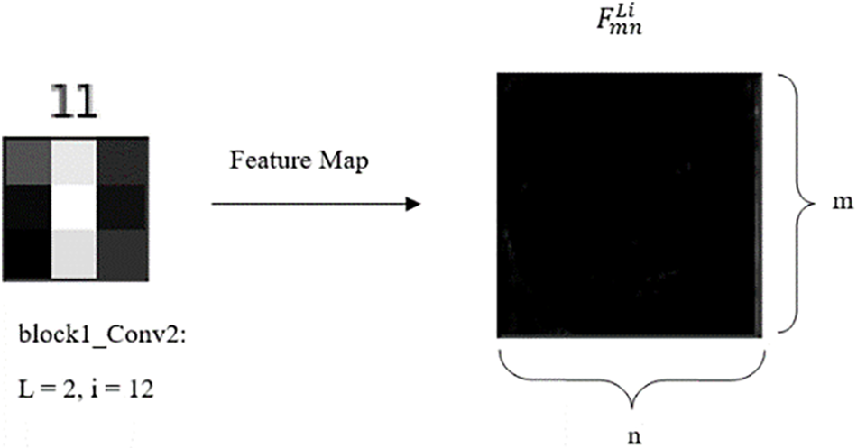
Figure 4: The feature map generated by a filter for the VGG 16 model, this feature map indicates that the corresponding filter is disabled and does not extract features

In Fig. 4, parameters (L) and (i) represent the index of the layer and the index of the filter, respectively. (m) and (n) represent the length and width of the feature map, which is usually (m) equal to (n). FmnLi represents the feature map associated with the i-th filter in the L-th layer of the model.

Sum(FmnLi)=Σi=1    MΣj=1    NFmnLi(1)

deactivated filter:Sum(FmnLi)=δ (0≤δ≤0.02)(2)

2.   When there is a correlation between 2 or more feature maps, and it fails to extract facial features. The correlation between the two feature maps indicates that the filters related to these feature maps extract similar information. As a result, removing these filters reduces the computational cost of the model without introducing any change in the model’s accuracy.

Fig. 5 illustrates the types of correlations that exist between two feature maps. As seen in this figure, in the proposed method, only feature maps that exhibit robust correlations with each other are eliminated, and only one of them is saved.

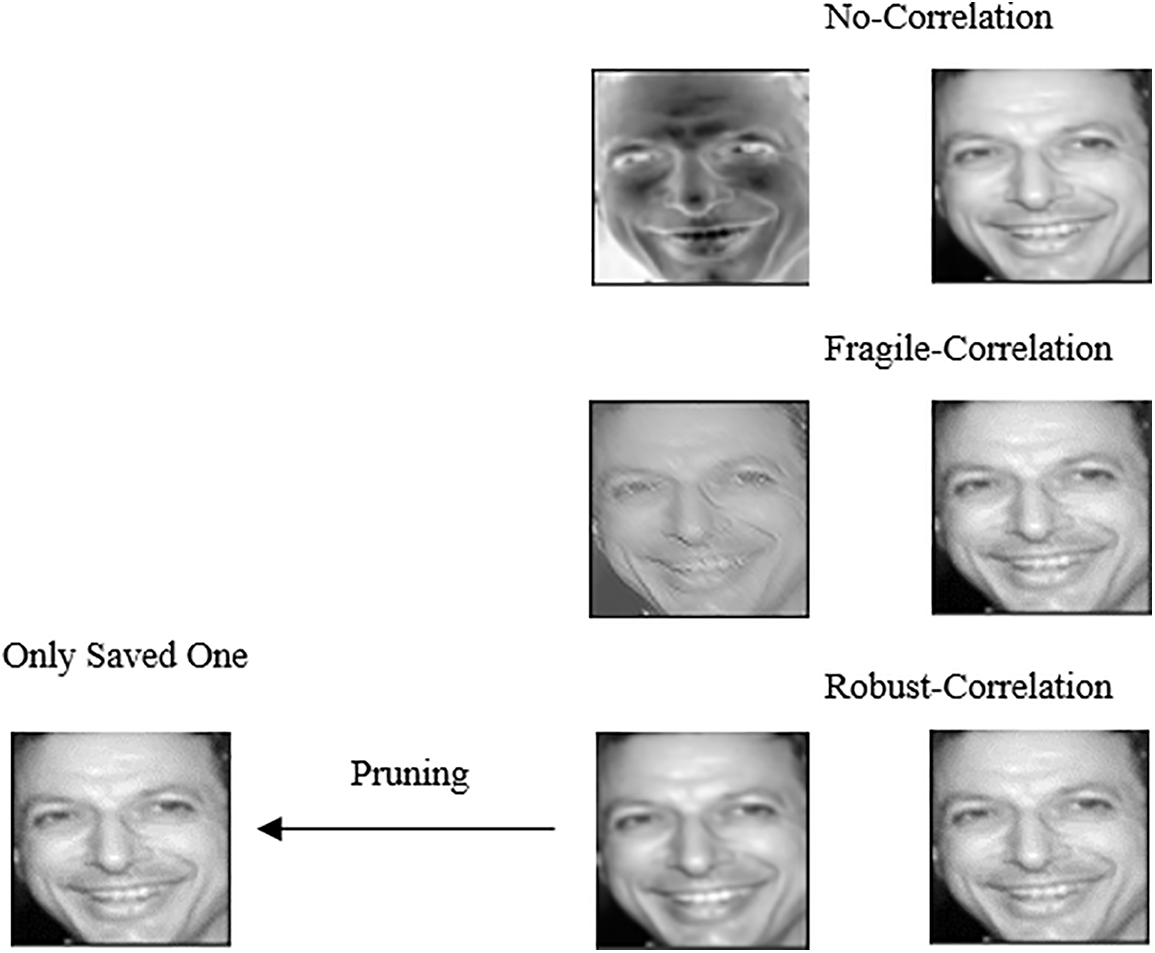
Figure 5: Types of correlation between two feature maps

FgLi set as the matrix of output feature map associated with the i-th filter in the L-th layer of the model, and FgLk is k-th matrix of output feature map of the same layer L, both the matrix converted into a vector of feature maps given below:

F^gLi=(F1Li,F2Li,F3Li,....,FgiLi)(3)

F^gLk=(F1Lk,F2Lk,F3Lk,....,FgiLk)(4)

NgLi=FgLi−ming{FgLi}Maxg{FgLi}−ming{FgLi}(5)

NLi=(N1Li,N2Li,…,NgiLi)(6)

For F^gLk:

NgLk=FgLk−ming{FgLk}Maxg{FgLk}−ming{FgLk}(7)

NLk=(N1Lk,N2Lk,…,NgiLk)(8)

After, for the L-th convolutional layer, the Pearson correlation of both i-th and k-th vectors of feature maps are given as:

ρ((NLi),(NLk))=∑g=1gi(NLi−NLi¯)(NLk−NLk¯)∑(NLi−NLi¯)2(NLk−NLk¯)2(9)

Let NLi¯ represent the mean of NLi, and NLk¯ represent the mean of NLk. The range of values for ρ((NLi),(NLk)) is from −1 to 1. If ρ((NLi),(NLk)) is 0, it indicates that NLi and NLk are independent; otherwise, the value is 1. The closer the value of ρ((NLi),(NLk)) is to 1, the higher the correlation between the two feature maps. In this method of identifying inactive filters, we empirically consider filters associated with feature maps whose correlation level is greater than 0.95 as possible filters that have been deactivated.

deactivated filter:ρ((NLi),(NLk))≥φ (φ=0.95)(10)

Now, for 100 selected samples, we identify and save the possible inactive filters by Eqs. (2) and (10). A filter is identified as deactivated if it is inactive for at least 80% of these samples.

Accordingly, deactivated filters were identified and removed from the model to construct a new structure with fewer parameters.

The pseudo-code of the proposed algorithm is presented in Fig. 6. The initial weighting of the model was carried out by the weights obtained by the ImageNet data set training. (D) is a subset of the CASIA-WebFace dataset containing Nd (= 82,494) samples of Cd (= 1,000) classes. β is the number of epochs where the model is fine-tuned on D. The value of β is empirically chosen to be 100. K is the dataset used for detecting inactive filters. Parameter (F) is a list of all filters in all convolution layers of the basic network. All filters detected as inactive are saved in (Z), in which (Zf) is the number of samples for which the specific filter (f) was passive. Parameter (α) is a threshold for the detection of inactive filters. The value of (α) was chosen to be 0.8 based on experiments. This means those elements of (Z) with 80% repetition for input (Nk) are recognized as inactive filters and saved in the dictionary (P). The elements of (P) are removed from (F). The remaining model is referred to as (M). The (M) is fine-tuned for (0.1* β) to assess its convergence, and if it converges, it will be saved as the final model and retrained for (2* β) epochs. If the remained model does not converge, the removed filters had a good impact on the whole network and should not be deleted. Therefore, a reconsideration of the amount of filter removal is necessary. It should be noted that this situation did not occur in our experiments.

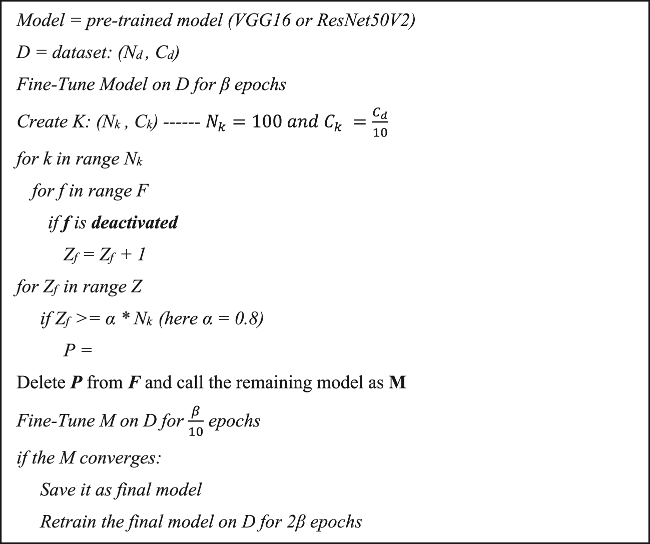
Figure 6: Pseudo-code of the proposed algorithm for network pruning

Fig. 7 shows the strategy of the proposed model to remove the filters from each block of the ResNet50V2 model. As authenticated here, each layer’s deleted filter ratio is independent of other layers. In similar methods such as ThiNet [13] (Fig. 2), the filter elimination rate was constant for each block or defined by a threshold value. Furthermore, the inactive filters were detected only for the first two layers in ThiNet. However, when the ResNet50V became more profound, the number of blocks and layers of each block increased, and our method could detect and remove inactive filters in all layers, except for the Addition layers. Detecting and eliminating inactive filters is significantly easier for the VGG16 network with sequential architecture and no concatenation layer.

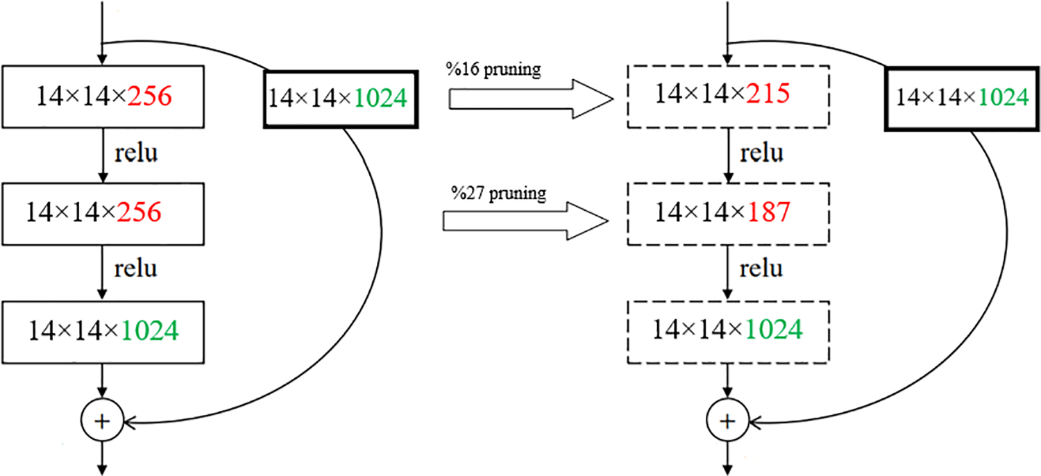
Figure 7: The proposed method strategy for removing filters in each block of the ResNet50V2 network

It is worth mentioning that negative data deactivates filters. A filter removed by negative data may contribute to the extraction of good features for positive data. To overcome this challenge, filters are not simply removed according to the result of a single training sample. For this purpose, deactivated filters are identified experimentally for 100 randomly selected samples, and then the filters identified as inactive for 80% of the data are removed. These 100 samples are chosen from 100 classes with the highest population.

4  Experimental Results

Deactivated filters are not only because of the ReLU activation function but also due to initial (pre-trained) weights. Weights obtained from pre-trained models by ImageNet are used to initialize weights in convolutional layers.

The ImageNet dataset consists of 1000 object classes, some of which bear no resemblance to human facial features. Thus, a certain number of filters fail to extract the appropriate features when feeding facial data to a model for training, making their feature maps black (all zero). This is most noticeable in higher layers, where more abstract features are extracted. For example, Fig. 8 shows that the first feature map generated by the corresponding filter (index 0) is entirely black. Accordingly, the proposed method identified this filter as deactivated and removed it.

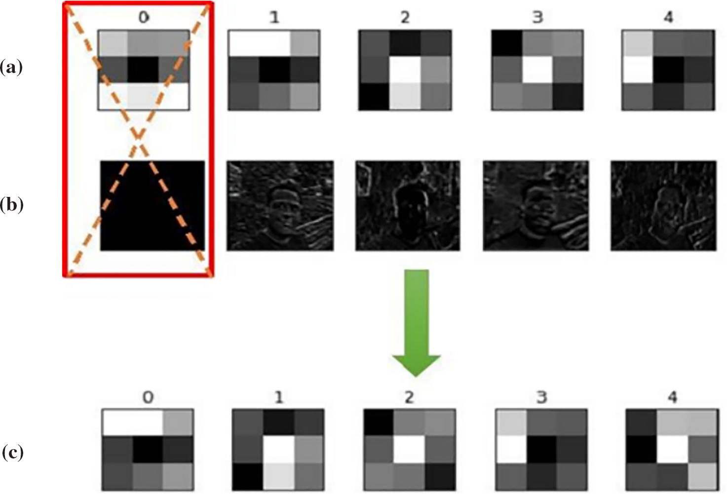
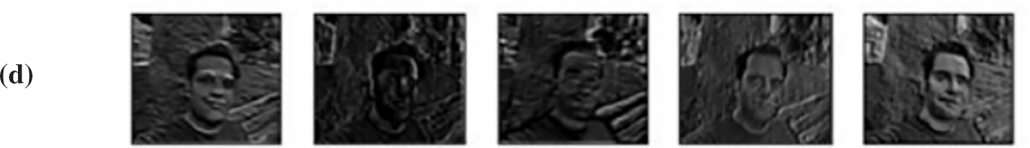
Figure 8: An example of network pruning. Top: First 5 feature maps of a layer from the initial model. Bottom: New feature maps after removing the inactive filter and training again

As shown in this figure, our proposed method removes the filter with an index (0) in the next step because it failed to extract the appropriate features. Filters 1–4 were found to be valid, so they were not released. After removing a filter, the next filter will be replaced, and this process continues until the completion of the identification process for inactive filters in a layer. Fig. 9 illustrates the process of filter removal and replacement in a layer.

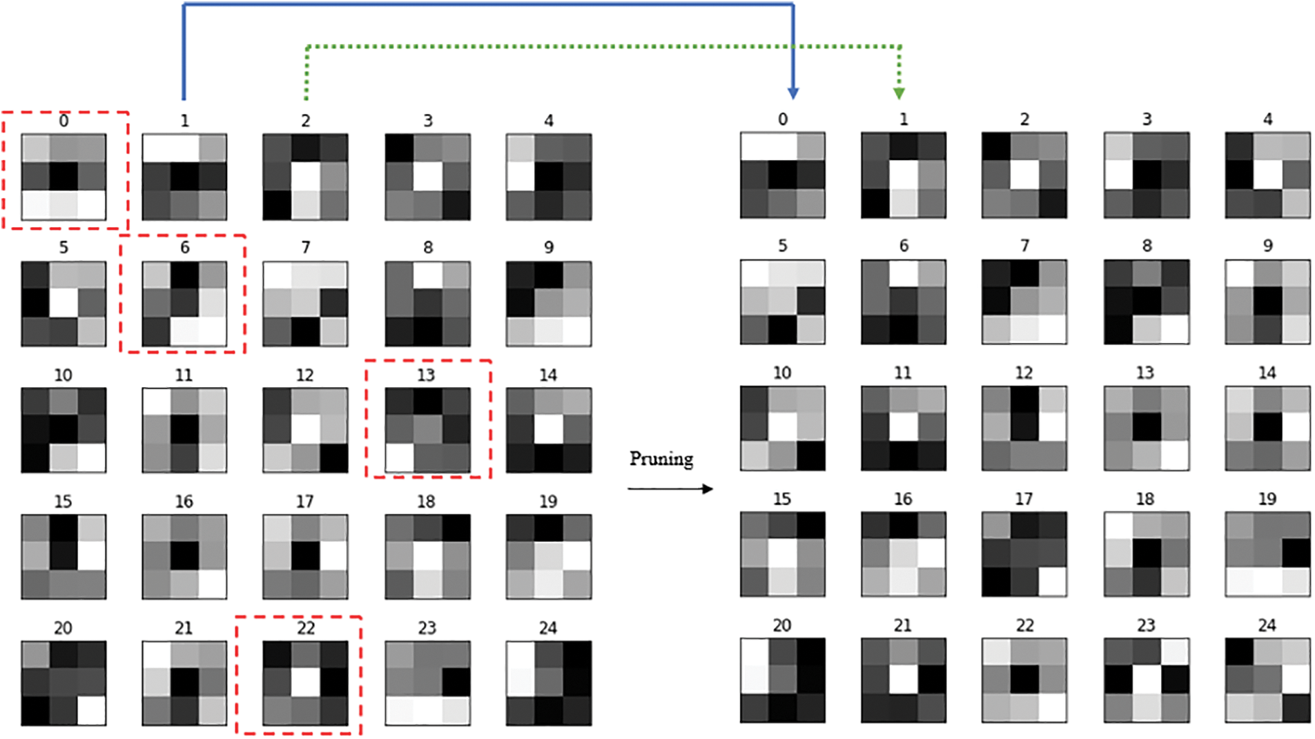
Figure 9: The process of removing and replacing filters in a layer. In this figure, the filters highlighted with a red box have been removed after the network pruning process. For example, the filter with index 0 has been removed, and the filter with index 1 has been replaced in its position

Fig. 10 illustrates the filters and their corresponding feature maps before and after the network pruning process. This figure showcases the filters and feature maps for a face recognition model with the VGG16 base architecture in the second convolutional layer.

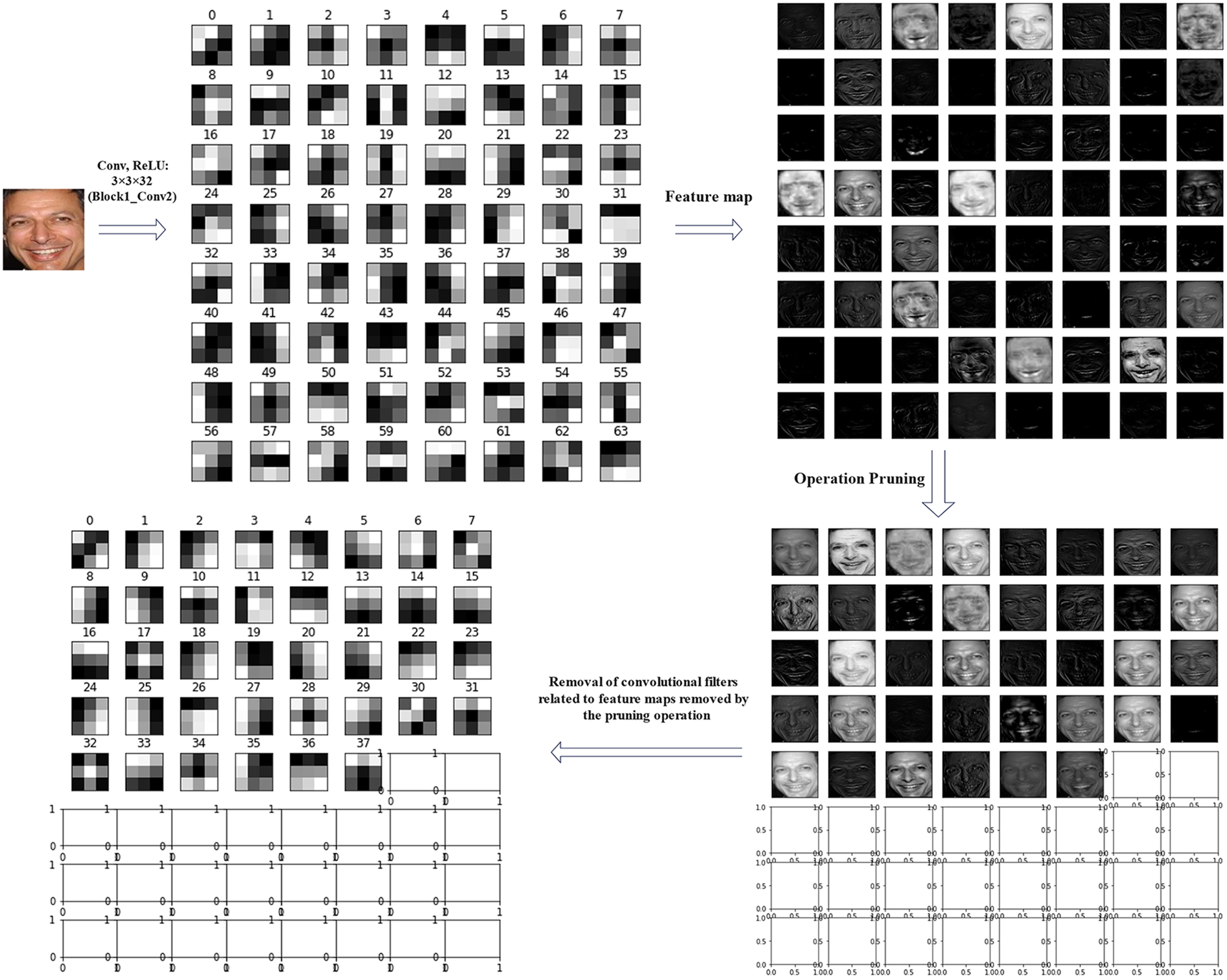
Figure 10: Filters and their corresponding feature maps before and after the network pruning process for the Face recognition model with the VGG16 base architecture VGG16

Figs. 11 and 12 depict the filters and feature maps generated by the initial and final models for models with VGG16 and ResNet50V2 backbones, respectively. A number of the developed feature maps generate no features, imposing computational costs on the model (Fig. 8b). This problem can be solved by identifying and removing deactivated filters.

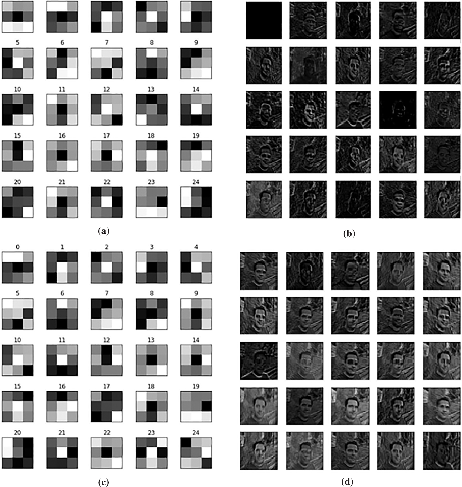
Figure 11: (a) Filters in the third convolutional layer of the VGG16 model, (b) Corresponding feature maps of a, (c) Filters in the third convolutional layer after deactivated filters are removed, (d) Corresponding feature maps of c

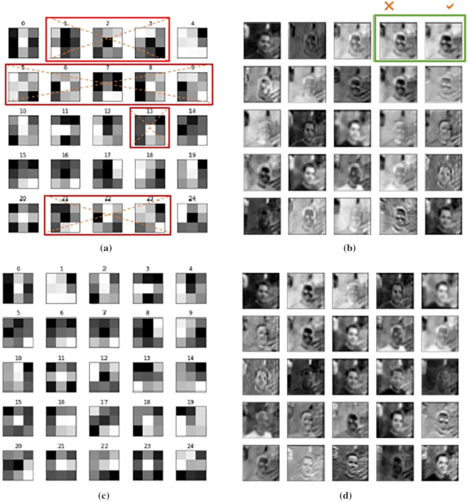
Figure 12: (a) Filters in the 34th convolutional layer of the ResNet50V2 model. Red boxes show inactive or useless filters. Some of them are selected based on their small gradients, and some of them (e.g., 3) produced the same feature maps, (b) Corresponding feature maps of a, (c) Filters in the 34th layer after deactivated filters are removed, (d) Corresponding feature maps of c

As shown in Fig. 12, for the model with the ResNet50V2 backbone network, the filters that produce similar feature maps are removed, and only one of them is retained, displayed in green boxes (e.g., filters 3 and 4). The filter with index 3 is removed, while the filter with index 4 is kept. The reason for removing the filter with index 3 was its high correlation with the filter with index 4. The filters that their feature maps had minor features have also been removed.

In Table 2, the performance of the proposed method on the VGG16 model is shown. In this model, the base network is VGG16, used to train the network on the CASIA-WebFace dataset. The LFW benchmark evaluates the performance of the model. The loss function in this model is Cross-Entropy. As shown in Table 2, the accuracy model has increased by 0.74% compared to the model in which the deactivated filters are not removed. In addition, our method reduced this model’s convolution parameters and FLOPs by 26.85% and 47.96%, respectively.

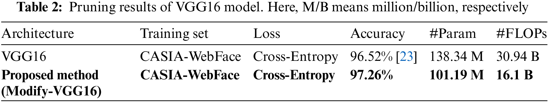
Table 3 shows the performance of the proposed method on pruning the ResNet50V2 model. This table compares the results obtained by our method with other methods. In the ResNet50V2 model, the Top-1 and Top-5 accuracies are 1.1% and 0.9% higher than the ResNet50 model on the ImageNet benchmark, respectively, while the number of parameters of the two models is the same [24]. The ArcFace model [25] was employed for face recognition using the base architecture ResNet50V2. According to the proposed method, deactivated filters were identified for this model. All models were trained with the CASIA-WebFace dataset. The LFW benchmark has evaluated the performance of the models. The accuracy of our proposed model has decreased by only 0.11% compared to the ArcFace model that used the basic architecture of ResNet50V2, which shows that our model has been able to maintain the accuracy of the original model. The proposed method achieves 2.34× FLOPs reduction and 2.46× compression on the ResNet50V2 model.

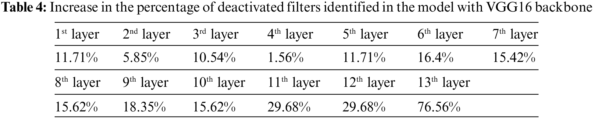
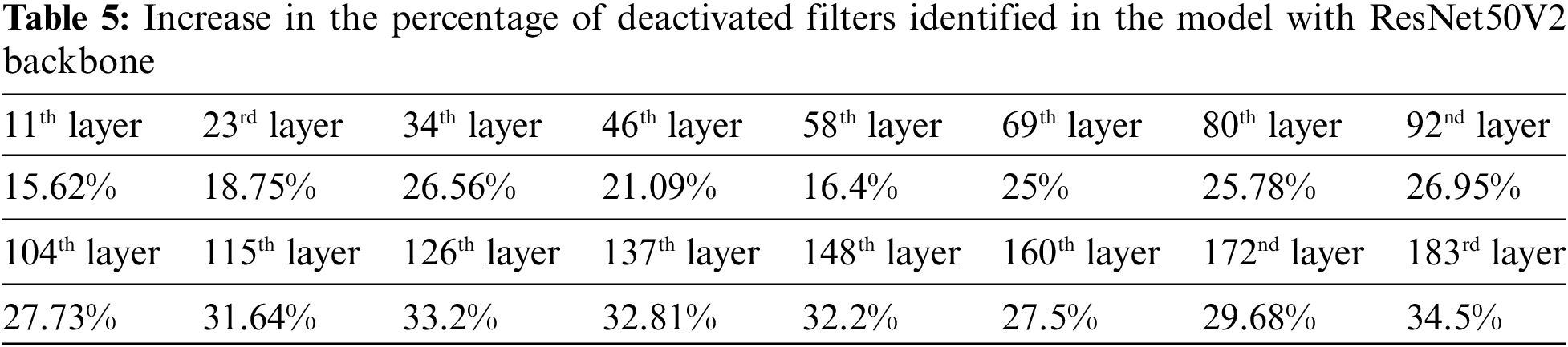
As previously mentioned, the weight initialization of models was carried out using pre-trained weights of the ImageNet dataset. The ImageNet has 1000 object classes, including caddy, Tower of Pisa, ice cream, etc. More deactivated filters are expected in the higher layers of the network for the face recognition model initialized via ImageNet and trained by face data. This is because, in a deep model, more abstract features are extracted in higher layers than in lower layers. So, the expectation is that these pre-trained models extract features in higher layers, and many of these features bear no resemblance to human facial features. Therefore, increasing the rate of deactivated filters identified by increasing the layer depth can be regarded as a criterion for measuring the accuracy of deactivated filter identification. Tables 4 and 5 list the percentage of deactivated filters identified in each layer for models with VGG16 and ResNet50V2 backbones, respectively.

5  Conclusions

In this paper, we assumed that if in the convolutional layers of the face recognition model, we identify and remove the filters that have been disabled due to the use of the ReLU activation function, we can reduce the redundancy in the model by maintaining the accuracy of the face recognition model. As a result, the final model will be compressed, and the training speed of the model will also increase. To investigate this hypothesis, we chose two face recognition models, one with VGG16 basic architecture and the other with ResNet50V2 basic architecture.

The reason for choosing these two models was to check the performance of the proposed method in sequential models (VGG16) and functional models (Resnet50N2). The proposed hypothesis was proved according to the obtained results. According to the results obtained in the face recognition model with VGG16 basic architecture, we improved the model’s accuracy by 0.74%; in addition, we reduced convolution parameters by 26.85%, and FLOPs decreased by 47.96%. For the face recognition model with ResNet50V2 basic architecture, we used the ArcFace method for face recognition; after removing the inactive filters in this model, the accuracy decreased by 0.11%, while the training speed of the model increased, and the convolution parameters of the model reduced by 59.38%. Moreover, the FLOPs of the model were also reduced by 57.29%. By utilizing our proposed method, the size of the face recognition model with the VGG16 base architecture was reduced from 500 to 150 MB, which is a significant achievement in this article. By integrating our proposed models with the SqNxt block, we anticipate a reduction in the parameters of the resulting model. This concept is suggested for future research.

Acknowledgement: The authors thank the Advanced Computing Research Laboratory, Faculty of Electrical Engineering, Shahrood University of Technology for their continued support and the supervisor for his guidance and constant support rendered during this work.

Funding Statement: The authors received no specific funding for this study.

Author Contributions: Conceptualization: Mostafa Diba; Methodology: Mostafa Diba, Hossein Khosravi; Formal analysis and investigation: Mostafa Diba; Writing—original draft preparation: Hossein Khosravi, Mostafa Diba; Writing—review and editing: Mostafa Diba, Hossein Khosravi; Funding acquisition: Hossein Khosravi; Supervision: Hossein Khosraviversion. All authors reviewed the results and approved the final version of the manuscript.

Availability of Data and Materials: The code of the paper is placed in the link below: https://github.com/mosdiba/Pruning-Networks-for-Face-Recognition. The dataset used in this article is CASIA-WebFace, which is available in link below: https://www.kaggle.com/datasets/debarghamitraroy/casia-webface.

Conflicts of Interest: The authors declare that they have no conflicts of interest to report regarding the present study.

References

1. M. T. H. Fuad, A. A. Fime, D. Sikder, M. A. R. Iftee, J. Rabbi et al., “Recent advances in deep learning techniques for face recognition,” IEEE Access, vol. 9, pp. 99112–99142, 2021. [Google Scholar]

2. R. Hammouche, A. Attia, S. Akhrouf and Z. Akhtar, “Gabor filter bank with deep autoencoder based face recognition system,” Expert Systems with Applications, vol. 197, pp. 116743, 2022. [Google Scholar]

3. K. Simonyan and A. Zisserman, “Very deep convolutional networks for large-scale image recognition,” arXiv preprint arXiv:1409.1556, 2014. [Google Scholar]

4. I. Bello, W. Fedus, X. Du, E. D. Cubuk, A. Srinivas et al., “Revisiting ResNets: Improved training and scaling strategies,” Advances in Neural Information Processing Systems, vol. 34, pp. 1–14, 2021. [Google Scholar]

5. D. Yi, Z. Lei, S. Liao and S. Z. Li, “Learning face representation from scratch,” arXiv preprint arXiv:1411.7923, 2014. [Google Scholar]

6. K. He, X. Zhang, S. Ren and J. Sun, “Identity mappings in deep residual networks,” in European Conf. on Computer Vision, Israel, Tel Aviv, Springer, pp. 630–645, 2016. [Google Scholar]

7. G. B. Huang and E. Learned-Miller, “Labeled faces in the wild: Updates and new reporting procedures,” Technical Report, Dept. Comput. Sci., Univ. Massachusetts Amherst, Amherst, MA, USA, vol. 14, no. 3, 2014. [Google Scholar]

8. S. Han, J. Pool, J. Tran and W. Dally, “Learning both weights and connections for efficient neural network,” Advances in Neural Information Processing Systems, vol. 28, pp. 1–9 2015. [Google Scholar]

9. S. Han, H. Mao and W. J. Dally, “Deep compression: Compressing deep neural networks with pruning, trained quantization and huffman coding,” arXiv preprint arXiv:1510.00149, 2015. [Google Scholar]

10. X. Dong, S. Chen and S. Pan, “Learning to prune deep neural networks via layer-wise optimal brain surgeon,” Advances in Neural Information Processing Systems, vol. 30, pp.1–11, 2017. [Google Scholar]

11. Y. He, G. Kang, X. Dong, Y. Fu and Y. Yang, “Soft filter pruning for accelerating deep convolutional neural networks,” arXiv preprint arXiv:1808.06866, 2018. [Google Scholar]

12. F. Tung and G. Mori, “CLIP-Q: Deep network compression learning by in-parallel pruning-quantization,” in Proc. of the IEEE Conf. on Computer Vision and Pattern Recognition, Salt Lake City, Utah, USA, pp. 7873–7882, 2018. [Google Scholar]

13. J. H. Luo, J. Wu and W. Lin, “Thinet: A filter level pruning method for deep neural network compression,” in Proc. of the IEEE Int. Conf. on Computer Vision, Venice, Italy, pp. 5058–5066, 2017. [Google Scholar]

14. H. Li, A. Kadav, I. Durdanovic, H. Samet and H. P. Graf, “Pruning filters for efficient convnets,” arXiv preprint arXiv:1608.08710, 2016. [Google Scholar]

15. P. Molchanov, S. Tyree, T. Karras, T. Aila and J. Kautz, “Pruning convolutional neural networks for resource efficient inference,” arXiv preprint arXiv:1611.06440, 2016. [Google Scholar]

16. K. Akyol, “Comparing of deep neural networks and extreme learning machines based on growing and pruning approach,” Expert Systems with Applications, vol. 140, pp. 112875, 2020. [Google Scholar]

17. N. T. Le, B. Vo, L. B. Nguyen and B. Le, “OWGraMi: Efficient method for mining weighted subgraphs in a single graph,” Expert Systems with Applications, vol. 204, pp. 117625, 2022. [Google Scholar]

18. J. Liu, B. Zhuang, Z. Zhuang, Y. Guo, J. Huang et al., “Discrimination-aware network pruning for deep model compression,” IEEE Transactions on Pattern Analysis and Machine Intelligence, vol. 44, no. 8, pp. 4035–4051, 2021. [Google Scholar]

19. Y. He, P. Liu, Z. Wang, Z. Hu and Y. Yang, “Filter pruning via geometric median for deep convolutional neural networks acceleration,” in Proc. of the IEEE/CVF Conf. on Computer Vision and Pattern Recognition, Long Beach, California, USA, pp. 4340–4349, 2019. [Google Scholar]

20. R. Yu, A. Li, C. F. Chen, J. H. Lai, V. I. Morariu et al., “Nisp: Pruning networks using neuron importance score propagation,” in Proc. of the IEEE Conf. on Computer Vision and Pattern Recognition, Salt Lake City, Utah, USA, pp. 9194–9203, 2018. [Google Scholar]

21. Y. Tang, Y. Wang, Y. Xu, Y. Deng, C. Xu et al., “Manifold regularized dynamic network pruning,” in Proc. of the IEEE/CVF Conf. on Computer Vision and Pattern Recognition, pp. 5018–5028, 2021. [Google Scholar]

22. Y. Guo, A. Yao and Y. Chen, “Dynamic network surgery for efficient DNNs,” Advances in Neural Information Processing Systems, vol. 29, pp. 1–9 2016. [Google Scholar]

23. M. You, X. Han, Y. Xu and L. Li, “Systematic evaluation of deep face recognition methods,” Neurocomputing, vol. 388, pp. 144–156, 2020. [Google Scholar]

24. Keras Applications, Keras Library, 2022. [Online]. Available: https://keras.io/api/applications/ (accessed on 03/11/2022). [Google Scholar]

25. J. Deng, J. Guo, N. Xue and S. Zafeiriou, “ArcFace: Additive angular margin loss for deep face recognition,” in Proc. of the IEEE/CVF Conf. on Computer Vision and Pattern Recognition, Long Beach, California, USA, pp. 4690–4699, 2019. [Google Scholar]

26. W. Liu, Y. Wen, Z. Yu, M. Li, B. Raj et al., “SphereFace: Deep hypersphere embedding for face recognition,” in Proc. of the IEEE Conf. on Computer Vision and Pattern Recognition, Honolulu, Hawaii, USA, pp. 212–220, 2017. [Google Scholar]

27. Y. Srivastava, V. Murali and S. R. Dubey, “A performance evaluation of loss functions for deep face recognition,” in National Conf. on Computer Vision, Pattern Recognition, Image Processing and Graphics, Hubballi, India, Springer, pp. 322–332, 2019. [Google Scholar]

28. F. Wang, J. Cheng, W. Liu and H. Liu, “Additive margin softmax for face verification,” IEEE Signal Processing Letters, vol. 25, no. 7, pp. 926–930, 2018. [Google Scholar]

29. J. Deng, Y. Zhou and S. Zafeiriou, “Marginal loss for deep face recognition,” in Proc. of the IEEE Conf. on Computer Vision and Pattern Recognition Workshops, Honolulu, Hawaii,USA, pp. 60–68, 2017. [Google Scholar]