K-Hyperparameter Tuning in High-Dimensional Space Clustering: Solving Smooth Elbow Challenges Using an Ensemble Based Technique of a Self-Adapting Autoencoder and Internal Validation Indexes

1  Introduction

Cluster analysis is one of the data mining tasks in high-dimensional space [1]. Clustering algorithms, which are used in cluster analysis, aim to group data points in a manner that ensures data points within the same cluster are similar to each other and significantly different from data points in other clusters [1,2]. k-means is one of the most popular partition-based clustering algorithms used in cluster analysis, known for its many advantages, such as scalability [3]. However, its performance heavily depends on selecting the optimal number of k-clusters, which is typically referred to as the k-hyperparameter value [4]. Defining this value in high-dimensional space clustering with the k-means algorithm has been a long-standing challenge and remains an intractable and open research issue [5]. Although the use of the traditional elbow curve has a long-standing literature as one of the most successful techniques applied to help identify the correct k-hyperparameter value, a smooth elbow generated by some datasets is one of its major limitations [6]. The GLA-BRA-180 dataset is an example of a dataset that produces a smooth elbow on the elbow curve. This makes it difficult to identify the correct value of the k-hyperparameter from the unclear elbow [7,8]. Several techniques have been developed to address the limitations of smooth elbow formations. The statistical metric-based new elbow point discriminant technique is one such method [8]. In this technique, the mean distortion degree returned by the elbow is standardized between zero and ten. Then, the standardized results are used to calculate the cosine angles that intersect the points on the elbow. The calculated cosine angles are then utilized to compute the intersection angles between these points. This is then used to find the correct k-hyperparameter value. However, with this method, there are still some inconsistencies in the generated k-hyperparameter values, especially with datasets of increased dimensionality [8]. Development of an improved k-hyperparameter tuning technique on a smooth elbow is therefore crucial. This research therefore, aims to develop an improved technique for k-hyperparameter tuning technique on a smooth elbow based on the analysis of these techniques. The new technique leverages the ensemble of a self-adapting autoencoder and internal validation indexes to improve the traditional elbow technique. The analysis of both the new and existing techniques is based on a similar set of four high-dimensional datasets and five evaluation metrics. The four high-dimensional datasets encompass various types, including text, images, video, and audio datasets. The five metrics include the Silhouette index, Dunn index, Davies Bouldin index, Calinski Harabasz index, and the run times. The newly developed technique complements the existing literature on k-hyperparameter tuning techniques for addressing the challenges of smooth elbow. The improved technique demonstrates superior performance across high-dimensional datasets, including text, audio, video, and image-based data.

The organization of this paper is as follows: In the second section, the related works on the existing k-hyperparameter tuning techniques for smooth elbow are discussed. The related works also include the discussion of the traditional elbow methods, dimensionality reduction methods used with high-dimensional k-means clustering, as well as popular evaluation metrics. In the third section, experimental research design and implementation are discussed, with a focus on the methodology, experimental design, hypothesis, and the new technique. The methodology is achieved through a pre-study, experimental design, and finally a system development methodology for the new technique. In the fourth section, the experimental results are analyzed and discussed. Finally, in section five, the conclusions and recommendations for future research are stated.

2  Related Works

This section focuses on providing background information on the architecture of the k-means algorithm, the traditional elbow method, dimensionality reduction methods, and evaluation metrics. The challenge of using the elbow method to identify the correct value of the k-hyperparameter, as well as its mathematical definition, is explored in the discussion of the traditional elbow method. This section also focuses on reviewing the k-hyperparameter tuning techniques used to address the challenges of smooth elbow detection. The structure of the high-dimensional datasets is also explored in further detail in this section. Lastly, this paper also discusses the popular metrics used to evaluate k-hyperparameter tuning techniques for solving the smooth elbow challenges.

2.1 K-Means Architecture

K-means is an iterative algorithm that aims to partition a dataset into a set of k non-overlapping groups of data points [9]. The k-hyperparameter is one of the most important hyperparameters to tune in k-means [10,11]. Tuning a machine learning model’s hyperparameters has a significant effect on its performance [12]. In this subsection, we explore k-clusters, k-hyperparameters, and the traditional elbow method used to identify the optimal value for the k-hyperparameter.

2.1.1 K-Means Clusters

The k-means clusters are the resulting data sub-groups generated by the popular unsupervised partitioning algorithm, known as the k-means clustering algorithm [13]. Cluster analysis using the k-means algorithm is an example of a k-means-based model that has been successfully applied in cluster analysis [14,15]. The k-clusters generated by these algorithms are usually composed of distinct non-overlapping groups of data points, aggregated together because they share specific similarities [16]. The data points within a particular cluster are similar, while the data points across different clusters are different [17]. Both the intra-cluster and inter-cluster data points are measured using a sum of squared distance-based metric [18,19]. For this reason, the original un-partitioned dataset is standardized to have a mean of zero and a standard deviation of one [20]. The number of k-clusters obtained is determined by the random initialization of centroids at the beginning of the k-means clustering algorithm [21,22]. For this reason, it is important to run the algorithm using several centroid initializations and then select the cluster result that has the lowest sum of squared distances [23–25]. The visualization of the k-means clusters is typically achieved using scatter plots [26,27].

2.1.2 K-Means Hyperparameters

Hyperparameters have a direct control over the behavior of a machine learning algorithm and significantly impact the performance of the model [28,29]. Some of the commonly used k-means hyperparameters include max_iter, init_method, n_int and n_clusters. The max_iter is the number of iterations that a k-means algorithm runs before convergence. The init_method is the method through which the algorithm selects its initial cluster centers. The n_int refers to the number of times the algorithm will be initialized, while the n_clusters parameter refers to the number of clusters that will be generated by the k-means algorithm [30,31]. The latter, n_clusters, also referred to as the k-hyperparameter value, is considered the most important hyperparameter in high-dimensional k-means clustering, with a relatively higher level of impact compared to the other hyperparameters [32]. The algorithm for “learning hyperparameter optimization initializations” is an example of a k-means based model that has shown that the hyperparameter k-value has a greater impact compared to other k-means hyperparameters [32].

2.1.3 Elbow Method

The elbow method is a technique for assisting in the identification of the optimal value for the k-hyperparameter from a given dataset, and it has been extensively discussed in the literature [33]. It involves plotting the average dispersion on the Y-axis as a function of the number of clusters (k) on the X-axis [33]. After plotting the curve, the elbow of the curve is identified as the optimal number of clusters, which is the correct value for the k-hyperparameter to be used in a specific dataset [34]. However, the elbow can either be distinct, with a clear elbow or non-distinct, without a clear elbow [35]. Fig. 1 below shows a clear elbow, while Fig. 2 shows an indistinct elbow.

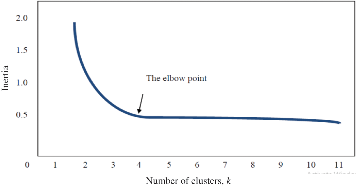
Figure 1: Distinct elbow method for selecting the optimal k clusters [35]

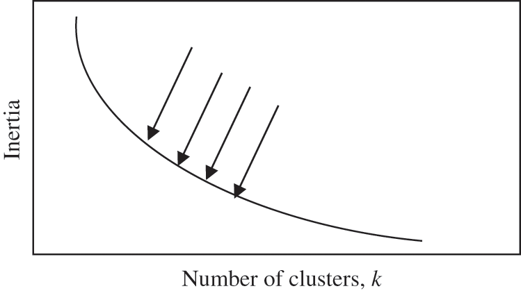
Figure 2: Example of non-distinct smooth elbow [36]

2.2 Mathematical Definition of Elbow

The reason for using a mathematical equation to define an elbow is because what may be considered a good elbow point in one situation may not be equally good in another situation. For this reason, authors have adopted the mathematical definition of curvature for a function as the basis for the mathematical formulation of an elbow point in an elbow curve [37]. This is defined as follows:

LF(K)=f″(k)((1+f′(k)2)3/2(1)

The elbow point, also referred to as the optimal number of clusters (k), is the point of highest curvature. It is a mathematical measure of the extent to which the function varies from a straight line. The maximum curvature is calculated by taking the derivative of the equation above and is considered the optimal value of k [37]. This derivative is stated as follows:

L′f(k)=f‴(k)(1+f′(k)2)−3 f″(k)2f″((k)2f′(k)=0(2)

2.3 High-Dimensional Datasets

The modern trends in technology have resulted in the generation of massive high-dimensional datasets [38,39]. The study of high-dimensional statistics has attracted immense interest from scholars and data scientists [40]. According to [41], a high-dimensional dataset is defined as a dataset where the number of features or attributes, P, is higher than or close to the number of instances or observations, N. This is in contrast to the misconception that a high-dimensional dataset is synonymous with big data, which consists of a large number of records [42,43]. For example, a dataset that has five features (P = 5) and four instances/data points (N = 4) would be considered a high-dimensional dataset, while a dataset with twenty thousand features (P = 20,000) and eighty thousand instances/data points (N = 80,000) would not be considered high-dimensional [44]. According to [45], it is most common to find high-dimensional datasets in the field of medicine [44,45]. An example is when there are a high number of attributes for a particular patient, such as body mass index, blood pressure values, diagnosis history, family history of illnesses, height, weight, and immune system status [46]. Fig. 3 below is an example of a high-dimensional dataset composed of several features for each patient.

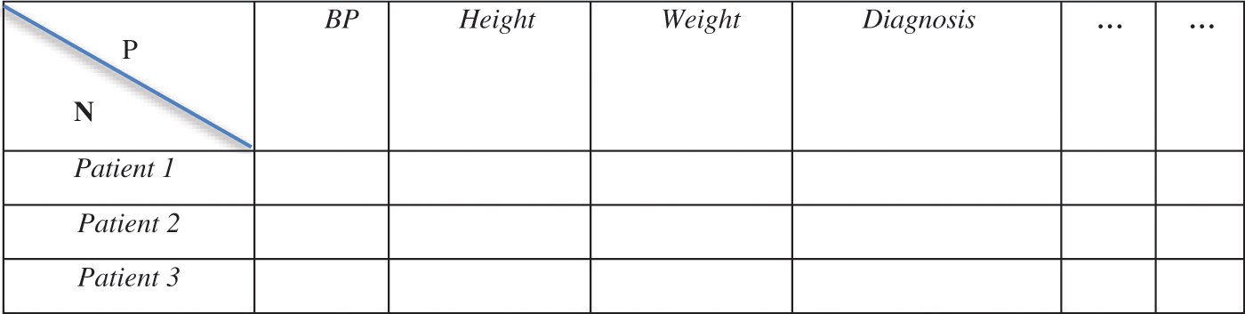
Figure 3: Example of a structure of high-dimensional dataset based on patients data [47]

In genomics and proteomic datasets, each sample can be defined by multiple measurements of up to a thousand or more [47,48]. Computational molecular medicine, computational anatomy, computational healthcare, computational neuroscience, and computational physiological medicine are some of the areas that have shown extensive use of high-dimensional datasets in cluster analysis [49]. Computational molecular medicine aims to construct a comprehensive understanding of molecular networks by gaining insights into the concentrations of biomolecules. Such assistance leads to more informed clinical decisions [50]. Computational physiological medicine aims to create disease models that integrate information from multiple levels of biological organization and apply these computational models to patient care. Such biological organizations include molecules, cells, tissues, and organ systems [50–52]. Computational anatomy aims to utilize mathematical theories to model anatomical structures and their variations in health and disease [53,54]. An example of computational anatomy is the identification of changes in the shape and motion of a heart, and using this data to predict specific cardiac diseases [55,56]. Computational healthcare integrates biomedical signal processing, computational modeling, machine learning, and health informatics to develop new strategies in personalized medicine. This is achieved through the analysis of e-health records, physiology-based time series data, and genomics [57–59]. Both computational molecular medicine and computational healthcare utilize a large number of high-dimensional datasets in their models [60–62]. The sparse and redundant nature of high-dimensional datasets poses great challenges for data scientists in data mining [63]. An “Enhanced Deterministic k-means Clustering Algorithm for Cancer Subtype Prediction from Gene Expression Data” is an example of a k-means-based computational medicine model that has been successfully applied in cluster analysis [64–67].

2.4 Dimensionality Reduction Methods Used in High-Dimensional K-Means

The dimensionality reduction methods are designed to transform data from a high-dimensional space to a low-dimensional space. This transformation, however, must aim to minimize information loss on the original high-dimensional dataset [68]. The methods for reducing data dimensionality are critical for improving the performance of high-dimensional k-means algorithms. Data dimensionality methods are categorized into both linear and non-linear methods. The most commonly used linear methods are Principal Component Analysis (PCA), Linear Discriminant Analysis (LDA), Singular Value Decomposition (SVD), and Factor Analysis (FA). On the other hand, the most commonly used non-linear data dimensionality reduction methods include kernel PCA, t-distributed Stochastic Neighboring Embedding (t-SNE), isomap embedding, multidimensional scaling (MDS), and Locally Linear Embedding (LLE). Data dimensionality reduction methods are useful for reducing the dimensionality of high-dimensional datasets, which present significant data mining challenges for data scientists [68]. In the following subsections, we will examine each of the unsupervised data dimensionality reduction methods in detail.

2.4.1 Principal Component Analysis

Principal Component Analysis (PCA) is a linear technique used to reduce the dimensionality of data. It aims to identify the most important low-level dimensions from a high-dimensional dataset while minimizing the loss of information from the original dataset [68]. It derives new linear variables from the original uncorrelated variables. Principal Component Analysis is calculated through eigen decomposition on the matrix of the data covariance. The obtained eigenvectors are similar to the principal axes of the maximum variance subspace. The eigenvalues show the variance of the inputs projected along principal axes. The number of significant eigenvalues indicates the approximate dimensionality. The size of the covariance matrix is similar to the dimensionality of the data. The Eigen decomposition strategy used by PCA can be computationally expensive, particularly in high-dimensional space. However, this method of reducing data dimensionality is simple to calculate and guarantees the generation of accurate representations of high-dimensional datasets in lower dimensions. The following is the formula for Principal Component Analysis (PCA) [69].

Projected Data=X∗PC(3)

where: Projected data is the transformed lower-dimensional representation of the original data. X is the standardized original data matrix, where each row corresponds to a data point, and each column corresponds to a feature. PC is the matrix of selected principal components, where each column represents a principal component (eigenvector).

2.4.2 Singular Value Decomposition

Singular Value Decomposition (SVD) is an unsupervised method used for reducing the dimensionality of data. It is applied to significantly reduce a large matrix to a smaller one, which is generated as the best rank k approximation. Singular value decomposition of matrix E is its factorization into three matrices product, i.e., E = UDVT. The U and V are the orthonormal columns, and the matrix D is diagonal with positive entries. The E data matrix is approximately a low-rank matrix. With the Singular Value Decomposition of matrix E, it is possible to obtain a matrix of rank k that provides the best approximation of E. Singular Value Decomposition is defined for both rectangular and square matrices, unlike the usual spectral decomposition in linear algebra. The left singular vectors, i.e., the columns of U, form an orthogonal set. The consequence of this orthogonality is that for a square and invertible matrix E, its inverse is formulated as VD-1UT. Outputs generated from the Singular Value Decomposition are usually dense, regardless of whether the supplied input is sparse or not [70]. The following is a formula for the Singular Value Decomposition (SVD):

X=U∗Σ∗V∧T(4)

where: U is an m × m matrix containing the left singular vectors (columns) that represent the relationships between the observations and the latent features. These vectors are orthogonal to each other and form an orthonormal basis for the row space of X. Σ is an m × n diagonal matrix containing the singular values (non-negative) along its diagonal. The singular values are sorted in descending order. They represent the importance of each latent feature (70). V^T is an n × n matrix containing the right singular vectors (rows) that represent the relationships between the features and the latent features. These vectors are orthogonal to each other and form an orthonormal basis for the column space of X [70].

2.4.3 Factor Analysis

Factor Analysis is a method for reducing data dimensionality that aims to reduce the original high-dimensional space by representing the entire matrix as a product of two smaller matrices, including random noise. Variables are modeled as linear combinations of the latent variables and the Gaussian error. Features are represented as factors, where the number of factors equals the number of features. When determining the number of factors (number of variables/features), a scree plot is generated with the Eigen function. This plot displays the original Eigen values and the common factor Eigen factors. The optimal number of factors, determined by analyzing the scree plot, is identified as the point where the Eigen values begin to level off, forming a plateau. The factor loadings heat map is used to visualize the most important variables/features from a high-dimensional dataset [70]. The formula for Factor Analysis is represented as follows:

X=µ+LF+ε(5)

where: X is the data matrix of observed variables. μ is the vector of means for each observed variable. LF is the matrix of factor loadings that represents the relationships between the observed variables and the latent factors. ε is the matrix of unique error terms. Fig. 4 below shows a scree plot used to identify the number of factors in the factor analysis data dimensionality reduction method.

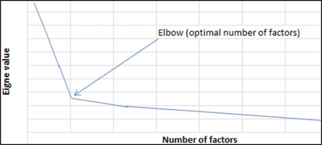
Figure 4: Scree plot to identify the number of factors in factor analysis method [70]

2.4.4 Isomap

Isomap is a multi-dimensional scaling-based unsupervised data dimensionality reduction method that estimates geodesic distances using shortest path distances. It then searches for the embedding of these geodesic distances in the Euclidean space. It represents high-dimensional space in a low-dimensional space by preserving the pairwise distances between points [71]. With data points, n, and a distance matrix E, Isomap computes the low-dimensional representation through Eigen decomposition of matrix E. Isomap aims to preserve the global structure and convert the original high-dimensional space into new coordinates, determined by the most significant eigenvectors [72].

2.4.5 Kernel PCA

Kernel PCA is an unsupervised data dimensionality reduction method and an extension of the popular Principal Component Analysis. The non-linear feature space is transformed into a linear feature space through the use of the kernel function. The inner product of the data points in the high-dimensional space is equal to the kernel matrix created by the kernel function. Any definite matrix with symmetric positive is said to be a kernel matrix [73]. Dimensionality reduction using kernel PCA is achieved through the Eigen decomposition process on the kernel matrix. It selects the most significant eigenvalues and eigenvectors of the kernel matrix to create a low-dimensional representation. Using kernel PCA, the computation of the high-dimensional feature space using kernels is a more efficient process than when using other methods for data dimensionality reduction [73,74]. The formula for projecting the original data onto the selected principal components (PC) can be represented as follows:

Projected Data=Centered_Kernel_Matrix∗PC(6)

where: Projected data is the transformed lower-dimensional representation of the original data. The Centered_Kernel_Matrix is the kernel matrix that has been centered to have a zero mean. PC is the matrix of selected principal components, where each column represents an eigenvector [74].

2.4.6 T-Distributed Stochastic Neighborhood Embedding (T-SNE)

T-SNE is an unsupervised data dimensionality reduction method that calculates the similarity between pairs of data points in both high-dimensional and low-dimensional spaces. Firstly, the similarities between data points in the high-dimensional space are measured using a Gaussian distribution. At this point, the first set of probabilities is generated. Secondly, the similarities between data points in the high-dimensional space are measured using the Cauchy distribution with one degree of freedom. At this point, the second set of probabilities in low-dimensional space is generated. Thirdly, t-SNE aims to accurately represent the set of probabilities in the high-dimensional space, ensuring that both mapping structures are as similar as possible. The difference between the two probability distributions is measured using the Kullback-Leibler divergence, commonly referred to as the KL-divergence. Finally, gradient descent is used to minimize the cost of the KL divergence [74].

2.4.7 Locally Linear Embedding

Locally Linear Embedding is an unsupervised nonlinear dimensionality reduction method that generates a low-dimensional representation while preserving the local structure of the high-dimensional space. This is achieved by exploiting the local symmetries of the linear reconstruction to uncover the nonlinear structure of the high-dimensional dataset. The local linear embedding maps its input into a single global coordinate system in the low-dimensional space, avoiding the need to consider local minima. Considering that the input data consists of d-dimensional vectors, the locally linear embedding (LLE) data dimensionality reduction method calculates the neighbors of each data point. The assumption is that the data points along the neighborhood lie on a locally linear manifold characterized by linear coefficients that have the capability to reconstruct each data point from the neighbors [74]. This is achieved by solving a weighted least squares problem, as shown in the equation below:

min∑(x_i−∑W_ij∗x_j)∧2(7)

W_ij

where: x_i is the data point to be reconstructed. x_j are the neighboring data points. W_ij are the weights that represent the linear combination coefficients.

The weights W_ij are constrained to satisfy certain conditions that ensure local linearity in the reconstruction. Weight Matrix: The weight matrix, W, is where each row corresponds to a data point, and each column contains the weights that represent the linear combination of its neighbors. The low-dimensional embedding is computed by solving an optimization problem that preserves the local relationships of the data points. This optimization aims to minimize the discrepancy between the pairwise distances in the high-dimensional space and the pairwise distances in the low-dimensional space for the neighboring data points using the formula below:

min∑(||z_i−z_j||−||x_i−x_j)∧2(8)

z_i, z_j

where: z_i and z_j are the low-dimensional embeddings of data points x_i and x_j, respectively.

2.4.8 Autoencoders

Autoencoders are a relatively new unsupervised method for reducing data dimensionality, based on feedforward neural networks. Their inputs are similar to the output. They have the capability to compress the input data into a lower-dimensional code and then recreate the output from this model. The code section of the autoencoder is a densely packed “summary” or “compression” of the input data. The close-packed summary is also referred to as the latent-space representation. Encoder, code, and decoder are the three components of an autoencoder. Subsequently, when building an autoencoder, three things are needed: a method for encoding, a method for decoding, and a loss function that compares the autoencoder’s output with the target. Mainly, autoencoders are used for dimensionality reduction. They have the capability to compress data effectively, in line with their training. They differ from standard data compression algorithms because they acquire knowledge from the specific attributes of the training data. The output of the autoencoder is not entirely identical to the input. However, it is close to it with a degraded representation. The process of training the autoencoder involves feeding the raw input data to it. Autoencoders do not require explicit labels during the training process. Instead, they generate their own labels from the training data [75]. It is represented by the following function:

z=f_encoder(x)(9)

where: X is the input data (e.g., a vector of features). Z is the encoding/representation of x in the latent space. f_encoder represents the mapping performed by the encoder neural network.

On the other hand, the decoder part of the autoencoder takes the representation of the latent space (encoding) and reconstructs the input data. It is represented by the following function:

x_hat=f_decoder(z)(10)

where: x_hat is the reconstructed data, which ideally matches the input data x. z is the representation of x in the latent space (encoding). f_decoder represents the mapping performed by the decoder neural network.

The autoencoder’s objective is to minimize the reconstruction error between the original input data x and the reconstructed data x_hat. This is usually measured using a loss function such as Mean Squared Error (MSE), shown below:

Loss=MSE(x,x_hat)(11)

The loss function quantifies how well the autoencoder can reconstruct the input data. During training, the autoencoder adjusts its parameters (weights and biases) using optimization techniques such as gradient descent to minimize the reconstruction error [75].

2.5 K-Hyperparameter Tuning Techniques Used to Solve the Challenges of Smooth Elbow

There are several techniques that have been proposed in the literature to solve the challenges of smooth elbows in the k-hyperparameter tuning process. The most popular ones include the L-method, Dynamic First Derivative Thresholding technique, New Elbow Point Discriminant technique, the Angle Based technique, and the Elbow Strength technique [76].

2.5.1 L-Method Technique

L-method places two straight lines on the elbow curve. One line extends from the head of the curve to the candidate point on the curve, while the other line extends from the tail of the curve to the candidate point on the same curve [77]. Using this technique, we first compute the Bayesian Information Criterion (BIC) values, as well as the first-order differences. The cosine angles between consecutive vectors formed by (k, BIC(k)) and (k+1, BIC(k+1)) are then computed. The point where the cosine angle shows a significant change is then identified. This is often indicated by a sharp decrease in the angle. The optimal value for the k-hyperparameter is determined by finding the intersection point of the two lines formed by the vectors before and after the change in angle in a given high-dimensional dataset. The pseudocode for this technique is represented as follows:

1. Initialize lists to store BIC, first-order difference and angles

     i)  bics = [ ]

    ii)  first_order_diff = [ ]

   iii)  angles = [ ]

2. Run the k-means algorithm for the current value of k

     i)  for k in range(1, max_k + 1):

    ii)  clusters, centroids = k_means(data, k, max_iterations)

3. Calculate the BIC for the current value of k

     i)  bic = compute_bic(data, clusters, centroids)

    ii)  bics.append(bic)

4. Calculate the first-order difference (except for the first element)

     i)  if k > 1:

    ii)  first_order_diff.append(bic - bics[−2])

5. Fit two straight lines to the head and tail of the curve

     i)  head_line = fit_straight_line(range(1, max_k + 1), bics, 0, max_k // 2)

    ii)  tail_line = fit_straight_line(range(1, max_k + 1), bics, max_k // 2, max_k)

6. Find the intersection point of the two lines

     i)  elbow_k = find_intersection(head_line, tail_line)

7. Plot the elbow curve, first-order difference and the fitted lines

     i)  plot_elbow_curve(range(1, max_k + 1), bics, first_order_diff, head_line, tail_line, elbow_k)

    ii)  def fit_straight_line(x_values, y_values, start_index, end_index):

8. Fit a straight line to a segment of the curve defined by start_index and the end_index

     i)  slope, intercept = linregress(x_values[start_index:end_index+1], y_values[start_index:end_index+1])

    ii)  return lambda x: slope * x + intercept

   iii)  def find_intersection(line1, line2):

9. Find the intersection point of the two straight lines

     i)  return (line2(0) - line1(0))/(line1(1) - line2(1))

However, with the L-method, long tails within the curve can influence the value of the optimal number of clusters, k [77]. To minimize this effect, a proposed iterative method aims to gradually decrease the tail while simultaneously refining the point of the elbow. The correct optimal cluster number, i.e., the value of the k-hyperparameter, requires multiple iterations [77]. This can be quite time-consuming and computationally expensive.

2.5.2 Angle Based Technique

The angle-based technique first calculates the measure of the Bayesian Information Criterion. After this, it calculates the first-order difference of the Bayesian Information Criterion. In order to determine the BIC values for various values of k (number of clusters) in the elbow curve, it is necessary to calculate the first-order difference of the Bayesian Information Criterion (BIC) and the BIC angle [78]. The Bayesian Information Criterion is given by the following formula:

BIC=log(n)∗k−2∗log(L)(12)

The “n” refers to the number of data points, “k” represents the number of clusters, and “L” denotes the likelihood of the data given the clustering model. The first-order difference of the BIC is calculated as the difference between consecutive BIC values for each k, and it is determined using the following formula:

First Order Difference=BIC(k)−BIC(k−1)(13)

The BIC angle is the angle between consecutive vectors formed by (k, BIC(k)) and (k+1, BIC(k+1)) in the BIC curve plot. It can help determine the point at which the BIC curve significantly changes its behavior, which may indicate the optimal number of clusters. The following is the pseudocode of this technique:

1. Compute the_bic (data, clusters, centroids):

     i)  n = len(data)

    ii)  k = len (data)

2. Compute the likelihood of the data given the clustering model

     i)  L = calculate_likelihood(data, clusters, centroids)

3. Compute and return BIC

     i)  Bic = math.log(n) * k − 2 * L

    ii)  return bic

4. Compute the likelihood

     i)  likelihood = 0

    ii)  for point, cluster_index in clusters.items():

   iii)  centroid = centroids[cluster_index]

5. Compute the log-likelihood assuming Gaussian distribution,

     i)  log_likelihood = −0.5 * sum((x - mu) ** 2 for x, mu in zip(point, centroid))

    ii)  likelihood += log_likelihood

   iii)  return likelihood

6. Initialize lists to store BIC, first-order difference, and angles

     i)  bics = [ ]

    ii)  first_order_diff = [ ]

   iii)  angles = [ ]

7. Run the k-means algorithm for the current value of k

     i)  for k in range(1, max_k + 1):

    ii)  clusters, centroids = k_means(data, k, max_iterations)

8. Calculate the BIC for the current value of k

     i)  bic = compute_bic(data, clusters, centroids)

    ii)  bics.append(bic)

9. Calculate the first-order difference (except for the first element)

     i)  if k > 1:

    ii)  first_order_diff.append(bic - bics[−2])

10. Calculate the angle for the current k (except for the first element)

     i)  if k > 1:

    ii)  angle = calculate_angle(k, bics[−2], k + 1, bic)

   iii)  angles.append(angle)

11. Plot the elbow curve, first-order difference, and angles

     i)  plot_elbow_curve(range(1, max_k + 1), bics, first_order_diff, angles)

12. Calculate the angle between (k1, bic1) and (k2, bic2) vectors

     i)  calculate_angle(k1, bic1, k2, bic2):

    ii)  vector1 = np.array([k1, bic1])

   iii)  vector2 = np.array([k2, bic2])

    iv)  dot_product = np.dot(vector1, vector2)

     v)  magnitude1 = np.linalg.norm(vector1)

    vi)  magnitude2 = np.linalg.norm(vector2)

   vii)  angle_radians = math.acos(dot_product/(magnitude1 * magnitude2))

  viii)  angle_degrees = math.degrees(angle_radians)

    ix)  return angle_degrees

The point with the biggest bayesian criterion angle is taken as the best approximate of the optimal number of clusters k [78]. However, there may be no clear point where the BIC curve changes in its behavior significantly. This technique, therefore, does not always guarantee the identification of the correct k-hyperparameter value from any given high-dimensional dataset.

2.5.3 Elbow Strength Technique

The elbow strength algorithm identifies the optimal number of clusters, k, by calculating the differences between the first and second order differences on the elbow curve. The concept of finite differences is used to calculate the differences between the first and second-order differences on the elbow curve. The first-order difference between consecutive points is calculated by subtracting the value at index i from the value at index i+1. The second-order difference is computed by taking the first-order difference between consecutive first-order differences. The point with the largest difference is referred to as the elbow strength and is considered the best approximation of the optimal number of clusters, the k-hyperparameter value [79]. The pseudocode for this technique is as follows:

1. Initialize empty list to store inertia for k’s

     i)  Inertias = [ ]

2. Run clustering for current k

     i)  For k in range(1, max_k + 1)

3. Run k-means algorithm for the current k-value

     i)  clusters, centroids = k_means(data, k, max_iterations)

4. Compute inertia for the current k-value

     i)  inertia = compute_inertia(data, centroids, clusters)

5. Append inertia to the list

     i)  inertias.append(inertia)

6. Compute first difference

     i)  first_diff = calculate_first_difference(inertias)

7. Compute second difference

     i)  second_diff = calculate_second_difference(first_diff)

8. Plot elbow and differences

     i)  plot_elbow_curve(range(1, max_k + 1), inertias, first_diff, second_diff)

9. Compute and return first difference

     i)  calculate_first_difference(values):

    ii)  first_diff = []

   iii)  for i in range(len(values) - 1):

    iv)  diff = values[i + 1] - values[i]

     v)  first_diff.append(diff)

    vi)  return first_diff

10. Compute and return second difference

     i)  calculate_second_difference(values):

    ii)  second_diff = [ ]

   iii)  for i in range(len(values) - 1):

    iv)  diff = values[i + 1] - values[i]

     v)  second_diff.append(diff)

    vi)  return second_diff

11. Plot elbow and pick the optimal k-value

12. End

However, this technique does not always guarantee the identification of the correct k-hyperparameter value from a given high-dimensional dataset.

2.5.4 New Elbow Point Discriminant Technique

The proposed technique is the New Elbow Point Discriminant, which is based on statistical metrics. In this technique, the mean distortion degree returned by the elbow is standardized between zero and ten. Then, the standardized results are used to calculate the cosine angles that intersect the points on the elbow. The BIC values and first-order differences are computed first. The cosine angles between consecutive vectors formed by (k, BIC(k)) and (k+1, BIC(k+1)) are then computed. The point at which the cosine angle exhibits a significant change is often marked by a sharp decrease in the angle. The point of intersection between the two lines formed by the vectors before and after the change in angle represents the optimal value for the k-hyperparameter. When using the computed cosine angles and their intersections to find the elbow point (optimal k-value), you are essentially looking for the “elbow” or “knee” in the plot where the angle between consecutive vectors changes significantly. The point where this change occurs represents the optimal k-value [80]. The pseudocode for this technique is as follows:

1. Calculate the BIC for the current value of k

     i)  bic = compute_bic(data, clusters, centroids)

    ii)  bics.append(bic)

2. Calculate the first-order difference (except for the first element)

     i)  if k > 1:

    ii)  first_order_diff.append(bic - bics[−2])

3. Calculate the angle for the current k (except for the first element)

     i)  if k > 1:

    ii)  angle = calculate_angle(k, bics[−2], k + 1, bic)

   iii)  angles.append(angle)

4. Find the elbow point using the cosine angles and their intersections

     i)  elbow_k = find_elbow_point(range(1, max_k + 1), angles)

5. Plot the elbow curve, first-order difference, and angles

     i)  plot_elbow_curve(range(1, max_k + 1), bics, first_order_diff, angles, elbow_k)

    ii)  find_elbow_point(k_values, angles):

6. Find the elbow point using the cosine angles and their intersections

     i)  max_angle_diff = 0

    ii)  elbow_k = 0

   iii)  for i in range(len(angles) - 1):

    iv)  angle_diff = angles[i] - angles[i + 1]

     v)  if angle_diff > max_angle_diff:

    vi)  max_angle_diff = angle_diff

   vii)  elbow_k = k_values[i + 1]

  viii)  return elbow_k

However, with this method, the computational cost is relatively higher. Moreover, this technique does not always guarantee the identification of the correct k-hyperparameter value.

2.5.5 Dynamic First Derivative Thresholding Technique

The Dynamic First Derivative Thresholding k-hyperparameter tuning technique is a hybrid technique composed of Menger curvature and L-method. The Dynamic First Derivative Thresholding technique approximates the first derivative of the curve, which is a local criterion that resembles the Menger curvature. The first derivative of the curve represents the gradient of the tangent line. Close to the operation of the L-method, the Dynamic First Derivative Thresholding technique aims to identify the region where the function has a sharp angle. The threshold algorithm is used to find the difference between high and low values of the first derivative, instead of fitting two straight lines. This categorizes the slopes into two groups: the head of the curve, which consists of high values, and the tail, which consists of low values. The point closest to the threshold is considered the elbow point [81]. This k-hyperparameter tuning technique on a smooth elbow can be represented with pseudo code as follows:

1.    Function dfdt (a, b)

2.    x ← f irstDerivative(a, b)

3.    y ← Data(m)

4.    tz ← 0

5.    minDist ← ||x [0] − y||

6.    for i ← 1;i < x.length;i + + do

7.    if ||x [0] − y|| < minDist then

8.    minDist ← ||x [0] − y||

9.    tz← i

10.   end if

11.   end for

12.   return tz + 1

13.   End function

2.6 Internal Validation Indexes for Evaluating Quality of Clusters in High-Dimensional K-Means

In clustering algorithms like k-means, there is no ground truth to accurately evaluate the model’s performance, as is the case with supervised algorithms. At the same time, there is no prior knowledge about the clustering dataset at hand. For this reason, it is important to use metrics that provide insight into the best or optimal value of k when clustering high-dimensional datasets [82]. Such a standard cluster validation process and set of internal validation metrics are highly critical for assessing the quality of the k clusters generated as the output. The optimal value of the k-hyperparameter in k-means determines the best clustering results. At this optimum, the variance within a cluster is normally low, while the separation between clusters is high [82,83]. The choice of internal validation metrics, as opposed to external and relative validation metrics, is based on the fact that internal validation metrics rely solely on the information inherent in the data itself. It is not based on prior information about the dataset [83]. The internal indexes are known to be better when applied in determining the quality of clustering results because they are solely based on the intrinsic information of the data alone [84]. The most commonly used internal validity metrics in the clustering literature include:

2.6.1 Dunn Index

The Dunn index, which is an internal validity metric, measures the level of compactness among objects within the same cluster and the level of separation between objects in different clusters [85]. The Dunn index is defined mathematically as follows:

DIm=1≤i≤j≤mMinδ(Ci,Cj)maxΔk1≤k≤m(14)

where distance between clusters i and j are denoted by δ (Ci, Cj) and the Δk is the size of cluster [85]. Higher values of the Dunn index indicate both the minimum intra-cluster distances and the maximum inter-cluster distance [85,86]. The k-means algorithm has successfully used the Dunn index to validate the clustering results it generates [86].

2.6.2 Calinski Harabsz Index

The Calinski-Harabasz index (CH), an internal validity metric, is defined as the ratio between the “sums of between-clusters dispersion” and “inter-cluster dispersion” for all clusters [87]. The Calinski-Harabasz index is defined mathematically as follows:

CI=tr(Bk)tr(Wk)∗Ng−kk−1(15)

WK=∑q=1k∑z∈Cq(x−Cq)(x−Cq)r(16)

Bk=∑q=1knq(Cq−CE)(Cq−CE)τ(17)

where k is the corresponding number of clusters, B(K) is the inter-cluster divergence, also called the inter-cluster covariance, W(K) is the intra-cluster divergence, also called the intra-cluster covariance, and N is the number of samples [87]. The larger the B(K) is, the higher the degree of dispersion between clusters. The smaller the W(K) is, the closer the relationship between the clusters [88]. Higher Calinski-Harabasz index values are better because they indicate good quality clustering performance and results [89].

2.6.3 Davies Bouldin Index

The Davies-Bouldin index (DB), an internal validity metric, is used to identify cluster overlap by measuring the ratio of the sum of the “within-cluster scatters” to the “between-cluster separations” [90,91]. The Davies-Bouldin index is defined as follows:

1k∑i=1kmaxj≠i(c¯i+c¯j∥wi−Wj∥2)(18)

A DB index close to zero (0) indicates that the clusters are compact and far from each other [92]. The implementation of the K-Medoids algorithm with Davies-Bouldin Index evaluation for clustering postoperative life expectancy in patients with lung cancer is an example of an algorithm that has applied the Davies-Bouldin index in its evaluation process [93].

2.6.4 Silhouette Index

The silhouette index is an internal validity metric that represents the optimal clustering number. It is calculated by taking the difference between the average distance within a cluster and the minimum distance between clusters [94–97]. The silhouette index is defined mathematically as follows:

s¯=1n∑i=1n(b(i)−a(i)max{a(i),b(i)})(19)

where a(i) represents the average distance of sample i to other samples in the cluster, b(i) represents the minimum distance of the sample from the sample i to the other clusters [97]. The algorithm that utilizes the silhouette index to determine the optimal k-means clustering on images in various color models is an example of the use of Silhouette index to evaluate quality of clustering results [97,98].

2.6.5 Bayesian Information Criterion (BIC)

Bayesian information criterion (BIC), an internal validity metric, is referred to as a strategy for model selection among a finite set of models. The model with the lowest BIC value is the most preferred, as it indicates good clustering results [99]. The Bayesian Information Criterion (BIC) index is calculated as follows:

BIC=2log(L)+qlog(L)(20)

L is the maximum likelihood function of the model and N is the number of data points in a dataset [99–101].

The inconsistent information provided by the various internal validation metrics/indexes is one of the challenges that render them unsuitable solutions when the elbow method fails. The silhouette index, for example, may generate the best score at a different optimal k-hyperparameter value than the best score generated by the Davies Bouldin index [101]. The effectiveness of each internal validation index/metric mentioned above is determined by the conditions present in a high-dimensional dataset. Each internal validation metric focuses on different aspects of the quality of the generated clusters. Comparing the scores of the various pairs of internal validation metrics for a single dataset, as well as assessing their consistency using Kendall’s index one at a time, would be computationally expensive. It is for this reason that we propose adopting an ensemble-based internal validation index in our approach to validate the quality of clusters from the high-dimensional k-means algorithm. The components of the ensemble internal validation index exercise equally sensitive to the varied conditions present in high-dimensional datasets. This type of ensemble could be based on either bootstrap aggregating (bagging) or boosting [101].

2.7 Ensemble Learning Techniques in Machine Learning

Ensemble techniques that train multiple base learners and then aggregate them, using methods such as bagging, stacking, and boosting, are considered state-of-the-art. It is widely recognized that ensembles have higher accuracy and performance compared to individual learners. Ensemble techniques are capable of enhancing weak learners into strong learners. Ensemble techniques have achieved significant success in various real-world tasks. Researchers from the fields of machine learning, data mining, and statistics have been extensively studying ensemble techniques from various perspectives, particularly in recent years. A number of ensemble techniques apply a single algorithm to generate homogeneous base learners, while other ensemble techniques apply several algorithms to generate heterogeneous base learners. Base learners can be created either in parallel or in a sequential manner. These base learners are then aggregated using a voting scheme for classification problems or using weighted averaging for regression problems [102]. The ensemble has been utilized in the development of the new k-hyperparameter tuning method for addressing the challenges posed by the smooth elbow.

3  Experimental Research Design and Implementation

This section describes the methodology utilized in the systematic review process, conducting main experiments as well as during the data analysis in this research. The main objective of this research work was to develop and validate an improved k-hyperparameter tuning technique for solving the challenges of smooth elbow in high-dimensional space clustering. The rest of this section is organized as follows: methodology, description of the high-dimensional datasets used in this experiment, experimental design, tools and data visualization, research objectives, hypothesis, and the metrics for evaluating the k-hyperparameter tuning techniques used to address the challenges of smooth elbows in high-dimensional space clustering. The proposed ensemble-based k-hyperparameter tuning technique using a self-adapting autoencoder and internal validation index is also discussed in this section.

3.1 Methodology for Review

A mixed methods research design was adopted in this paper, with a general focus on the positivist research philosophy. Qualitative research design entailed conducting a literature review on the existing k-hyperparameter tuning techniques for a smooth elbow. This qualitative research design also involved the utilization of design science methodology. Using the design science methodology, this research aimed to solve the problem of k-hyperparameter tuning on a smooth elbow through the design of a new technique. Quantitative research design, on the other hand, involves collecting and analyzing the results from the main experiments using an experimental design methodology. A similar set of high-dimensional datasets and evaluation metrics was used in the validation process. The high-dimensional datasets included a variety of data types, such as text, images, video, and audio. The process of developing a new technique adopted a multi-methodological design approach. The experimental design in this work demonstrates how all the experiments in this empirical study are carried out.

The systematic review process of the k-hyperparameter tuning techniques used to solve the challenges of smooth elbows in high-dimensional k-means clustering algorithms followed the five-step methodology as proposed by Khan, Kunz, Kleijnen, and Antes. This five-step methodology is applied when conducting a critical review of the existing literature [103]. The five-step methodology involves framing the questions for the review, identifying relevant literature, assessing the quality of articles, and reviewing the relevant literature. The meta-search-based strategy for identifying relevant literature focuses on k-hyperparameter tuning techniques to address the challenges of smooth elbows in high-dimensional k-means clustering algorithms.

3.2 Description of the High-Dimensional Datasets

Based on a purposive sampling strategy, the high-dimensional datasets used in this research study include the GLA-BRA-180 dataset, the Lung Cancer dataset, the YouCook dataset, and the COVID-19 coughs dataset. These datasets cover the four main categories of data: text, image, video, and audio. The GLA-BRA-180 dataset is text-based, the Lung Cancer dataset is image-based, the YouCook dataset is video-based, while the COVID-19 coughs dataset is an audio-based dataset. The GLA-BRA-180 dataset comprises 180 instances, 4,915 attributes/features, and 4 optimal clusters. This dataset involves the analysis of gliomas of different grades in computational medicine. The dataset is an expression profile of stem cell factors that are important in determining tumor angiogenesis. Glioma is the growth of cells from the brain or spinal cord. Glioma cells are similar in appearance to healthy glial cells. Glial cells surround the nerve cells and assist in their functioning [104]. When the glioma grows, it forms a mass of cells. Several types of gliomas can cause varying symptoms in different individuals, such as headaches, seizures, irritability, vomiting, visual difficulties, weakness, and numbness [104]. The GLA-BRA-180 dataset was initially downloaded as a .mat file but was later converted to a .csv file using both the scipy and pandas Python libraries.

The YouCook video-based dataset is a well-known benchmark dataset in computer vision. YouCook dataset focuses on the role of action recognition and anticipation in videos that involves cooking. The dataset has a huge database of instructional cooking videos together with their associated annotations. The YouCook dataset comprises 2,000 cooking videos, with each video demonstrating a step-by-step process of making a recipe. These videos are created from YouTube and cover a great variety of recipes and styles of cooking these recipes. The dataset comprises of different ingredients, cooking techniques, and culinary actions. Action labels have each action within the video labeled with a descriptive action name. These labels specify the type of action being performed in the corresponding video segment [105]. COVID-19 coughs datasets is an audio data, including cough sounds, to aid in the detection and diagnosis of COVID-19. Also referred to as COUGHVID, this dataset consists of more than 25,000 cough recordings from patients of different age-groups, gender and geographical locations. This dataset has been successfully used in clustering patients as either COVID-19 positive or negative [106]. Lung cancer dataset is a computational medicine dataset based on images and comprises of clinical attributes, i.e., patient age, history of smoking, and tumor characteristics. This also comprises of the target variable showing whether the patient suffers from lung cancer or not. Lung cancer dataset consists of 12,533 features, 181 instances and 2 clusters. It consists of radiological imaging features extracted from Computed Tomography scans and genetic mutation data. This dataset also comprises of clinical information on patient demographics, tumor characteristics, genetic markers, and treatment outcomes. Researchers use this dataset to investigate risk factors, create diagnostic models, predict the response of a particular treatment, and identify biomarkers associated with lung cancer [107].

3.3 Experimental Design, Tools and Data Visualization

According to [108], a proper design of experiments goes a long way in obtaining measurements that answer research objectives and/or hypotheses in a valid and efficient manner. The four high-dimensional datasets were each subjected to k-hyperparameter tuning techniques on a smooth elbow. The performance and statistical metrics were recorded for each run. An improved autoencoder was employed as the method for reducing data dimensionality, along with the existing k-hyperparameter tuning techniques. The scores of the metrics after each run are recorded and documented in a results table. The analysis of these results was followed by the formulation of conclusions and recommendations based on the hypothesis.

3.3.1 Research Objectives

In this paper, the research objectives were formulated as follows:

•   Evaluate the current k-hyperparameter tuning techniques used to address the challenges of smooth elbow.

•   Develop a new k-hyperparameter tuning technique to address the challenges of smooth elbow detection, utilizing an ensemble-based approach, combining a self-adapting autoencoder with internal validation indexes.

•   Validate the newly developed technique.

3.3.2 Research Hypothesis

In this paper, both the null hypothesis (H0) and the alternate hypothesis (H1) have been formulated in the subsequent sections as follows:

H0: There is no statistically significant difference between the performance of the newly developed k-hyperparameter tuning technique and the existing techniques used to address the challenges of a smooth elbow in high-dimensional space clustering.

H1: There is a statistically significant difference between the performance of the newly developed k-hyperparameter tuning technique and the existing techniques used to address the challenges of a smooth elbow in high-dimensional space clustering.

3.3.3 Tools of Experiment and Visualization

The Jupyter Notebook, Python’s IDE, was used to implement the new k-hyperparameter tuning technique proposed in this paper. TensorFlow, Keras Tuner, and Random Search were the main autoencoder libraries used with the new technique. The Matplotlib library was used for visualization, while the R software was used for computing the statistical scores. Spreadsheets were used to create charts.

3.3.4 Evaluation Metrics

Different performance and statistical metrics have been applied to compare various k-hyperparameter tuning techniques for addressing the challenges of smooth elbows in high-dimensional space clustering [109]. These metrics include the silhouette index, Calinski-Harabasz index, Dunn index, Davies-Bouldin index, as well as the run-time. The four internal validation indexes are commonly used metrics for evaluating the quality of clusters in high-dimensional space clustering [110]. Clustering accuracy is not a reliable metric for evaluating unsupervised learning tasks in machine learning. This is because there are no ground truth labels available to directly calculate accuracy. Moreover, the decision to use internal validation indexes instead of external cluster validation indexes is based on the fact that internal metrics for validating clusters rely solely on the inherent information within the data [111]. On the other hand, the decision to use the ensemble internal validation metric is based on the fact that all components of the ensemble validation index are equally sensitive to the diverse conditions present in a high-dimensional dataset. On the other hand, Cochran’s Q-score, McNemar’s score, and ANOVA were the statistical metrics applied in testing the hypothesis. Several statistical metrics exist in the literature on the hypothesis testing process of machine learning algorithms [112]. In this research, Cochran’s Q test [113] was used to determine whether there is a statistically significant difference in the optimal k hyperparameter values generated across the different k-hyperparameter tuning techniques on the GLA-BRA-180 dataset. MC Nemar’s score [114] was used to determine if there was a statistically significant difference in the k-hyperparameter value before and after the autoencoder compression process on any high-dimensional dataset, specifically the GLA-BRA-180 dataset. Anova [115] was used to investigate whether there was a statistically significant difference between the performance of the existing techniques and the new technique in solving the challenges of a smooth elbow.

3.3.5 Improved K-Hyperparameter Tuning Technique on a Smooth Elbow

The new and improved k-hyperparameter tuning technique on a smooth elbow is based on an ensemble-based self-adapting autoencoder. In this technique, a high-dimensional dataset first undergoes a compression process using a self-adapting autoencoder to generate a set of the most important features. The process of compressing data using an autoencoder is known as the encoding process. The architecture of the flexible autoencoder adapts itself in response to the type of high-dimensional data input. The engine’s ability to adapt itself based on the characteristics of the high-dimensional dataset input requires adjustments to several crucial hyperparameters. These hyperparameters include the number of hidden layers, the number of nodes, the choice of activation function, the choice of loss function, the learning rate and optimization method, regularization, batch size, number of epochs, initializer, learning rate schedule, dimensionality’s bottleneck dimensions, batch normalization, and early stopping. The new k-hyperparameter tuning technique aims to improve the autoencoder by combining the best set of hyperparameter settings based on the nature of the high-dimensional input dataset. The new k-hyperparameter tuning technique was implemented using Python version 3.6 and TensorFlow version 2.0. The autoencoder technique consists of three main libraries: TensorFlow, Keras Tuner, and Random Search. Keras Tuner was installed using the pip command, while the TensorFlow library was installed using the import function. TensorFlow library provides an application interface for the improved autoencoder, which incorporates the new k-hyperparameter tuning technique. Keras Tuner library automates the process of selecting the best combinations of hyperparameter settings to a great extent. Random search assists in sorting the different combinations of hyperparameter settings. These hyperparameter settings are defined in various function models. After importing the high-dimensional dataset input into the improved autoencoder, several model building functions are created. Different model building functions consist of a different set of hyperparameter settings. The best set of hyperparameter settings from these model functions is selected using Random Search. During the tuning process, both the maximum number of trials and the number of executions per trial are determined. Once the optimal combinations of hyperparameter settings are identified, the technique utilizes these settings to project a high-dimensional dataset into the latent space. This information is part of the decision that the technique uses to identify the correct k-hyperparameter value for a specific dataset. The validation score of the ensemble from the clustering result determines whether the autoencoder will make further internal adjustments or if the algorithm will stop if the scores are relatively the best. In clustering different high-dimensional datasets, the careful design of an architecture that can effectively learn and represent the underlying structure of a particular dataset is critical to the success of developing the new k-hyperparameter tuning technique. The carefulness in the design also incorporated the use of experimentation to find the optimal architecture and parameters for high-dimensional space clustering on a specific dataset.

In designing the image dataset handling system, the image data is normalized to a common scale during the data preprocessing stage. At the same time, the images are flattened or reshaped into a vector that is suitable for inputting into the autoencoder. The architecture’s depth was set to strike a balance between capturing more complex features from an image dataset and minding the computational constraints. Convolutional layers are used for both the encoder and the autoencoder because of their ability to capture spatial hierarchies. The hyperparameter settings were experimented with the RELU, Leaky RELU, and Swish activation functions. The incorporation of batch normalization layers was done to stabilize training and enhance convergence. The Kullback-Leibler Divergence was adopted as the loss function because it encourages the encoder to generate embeddings that are suitable for clustering. A regularization term was also added to enforce a compact clustering-friendly space. The combined reconstruction and clustering losses were minimized, while the learning rate and early stopping were used to improve training stability and convergence. During training, both the loss and the internal validation index scores were monitored to prevent over fitting.

In designing the text dataset handling process, the numerical features were standardized to ensure that they have similar scales. This can improve the training and clustering process during data pre-processing. The data pre-processing also involved appropriately handling any missing values, either by imputing them or encoding them as a separate category. The architecture consists of multiple encoding and decoding layers, utilizing fully connected components for both the encoder and the decoder. Dropout and L1 and L2 regularization techniques were used to prevent over fitting. The architecture design also experimented with three activation functions: ReLU, Leaky ReLU, and Scaled Exponential Linear Units (SELU). Mean Squared Error (MSE) was used for the reconstruction loss due to its popularity in such applications. Experiments were conducted to explore various regularization techniques aimed at incorporating a regularization term that promotes the suitability of the learned embeddings for clustering. The autoencoder was trained to minimize the reconstruction loss while also regularizing the embeddings. In order to improve training performance, learning rate scheduling and early stopping techniques were used. Depending on the complexity of the dataset, the changes in architectural designs and other hyperparameter settings were made based on the evaluation of the internal validation index scores of the clustering results. They were also based on different layer configurations, loss functions, and regularization techniques. Random search was used to find the optimal hyperparameters.

In developing the design for handling audio datasets, the motivation was to create an architecture that can efficiently capture the distinct patterns and characteristics present in audio data, thereby improving clustering performance. During the pre-processing stage, audio files were converted into spectrograms or other suitable representations that capture the frequency and time-domain characteristics of the audio signals. The spectrograms were also normalized to a standardized scale. In order to enhance the diversity of the training data, data augmentation techniques were implemented. The architectural design was tailored for audio data. Convolutional layers were used to capture local patterns and hierarchical features in the spectrogram data. Pooling convolutions were included to reduce the spatial dimensions while preserving important features. The experiment process utilized skip connections and the U-Net architectures to enhance feature preservation. The Mean Squared Error (MSE) between the input spectrogram and the reconstructed spectrogram was used as the reconstruction loss. Kullback-Leibler Divergence was used as the loss function as it encourages the encoder to produce embeddings that are friendly to clustering. The training strategy combined loss focuses on minimizing the reconstruction error and encouraging clustering-friendly embeddings. During training, the use of audio-specific data augmentation was considered the best option as it increased the robustness of the model. The fine-tuning strategy involved the experimentation process with various audio preprocessing techniques, architectures, and loss combinations. The specific audio pre-processing steps incorporated the application of Mel-frequency Cepstral coefficients (MFCCs) to enhance the quality of the input data.

In designing the architecture for handling video datasets, the goal was to create a system that can effectively capture both the temporal and spatial features present in video data. This would enable improved capturing of motion information and enhance clustering performance. The video frames were converted into suitable representations such as image frames, optical flow, or spatiotemporal volumes. The data preprocessing involved normalizing the pixel values to a common scale. Both random cropping and flipping were used as data augmentation techniques to increase the diversity of the training data. A 3D architecture, consisting of a convolutional autoencoder, was used to capture both the spatial and temporal features of video data. The convolutional layers were incorporated for spatial processing, while the recurrent layers were incorporated for temporal processing. Kullback-Leibler Divergence was used as the loss function because it encourages the encoder to generate embeddings that are conducive to clustering. The training strategy incorporated frame skipping and temporal jittering techniques to enhance temporal diversity. Fine-tuning was accomplished through iterations on the various hyperparameters, as well as an experimentation process involving different video pre-processing techniques. It also involved an evaluation process against the internal validation scores of the clustering results. In order to improve the quality of input data, the optical flow estimation technique was incorporated.

Using this technique, the optimal number of clusters, k, is determined through the bagging ensemble’s voting scheme. It is a trade-off between the number of clusters visualized in the autoencoder’s latent space and a k-value that has a relatively good score on the internal validation metric. Additionally, the k-value should generate a value of 0 or close to 0 on the derivative f‴(k)(1+f′(k)2)−3 f″(k)2f″((k)2f′(k). The ensemble validation metric discussed in the last paragraph of Section II was used to validate clusters in this technique. The discovery of the intrinsic structure of high-dimensional data, achieved through the adjustment of the flexible architecture of the autoencoder, is critical to the performance of the new k-hyperparameter tuning technique. Fig. 5 below shows the architecture of the newly developed k-hyperparameter tuning technique.

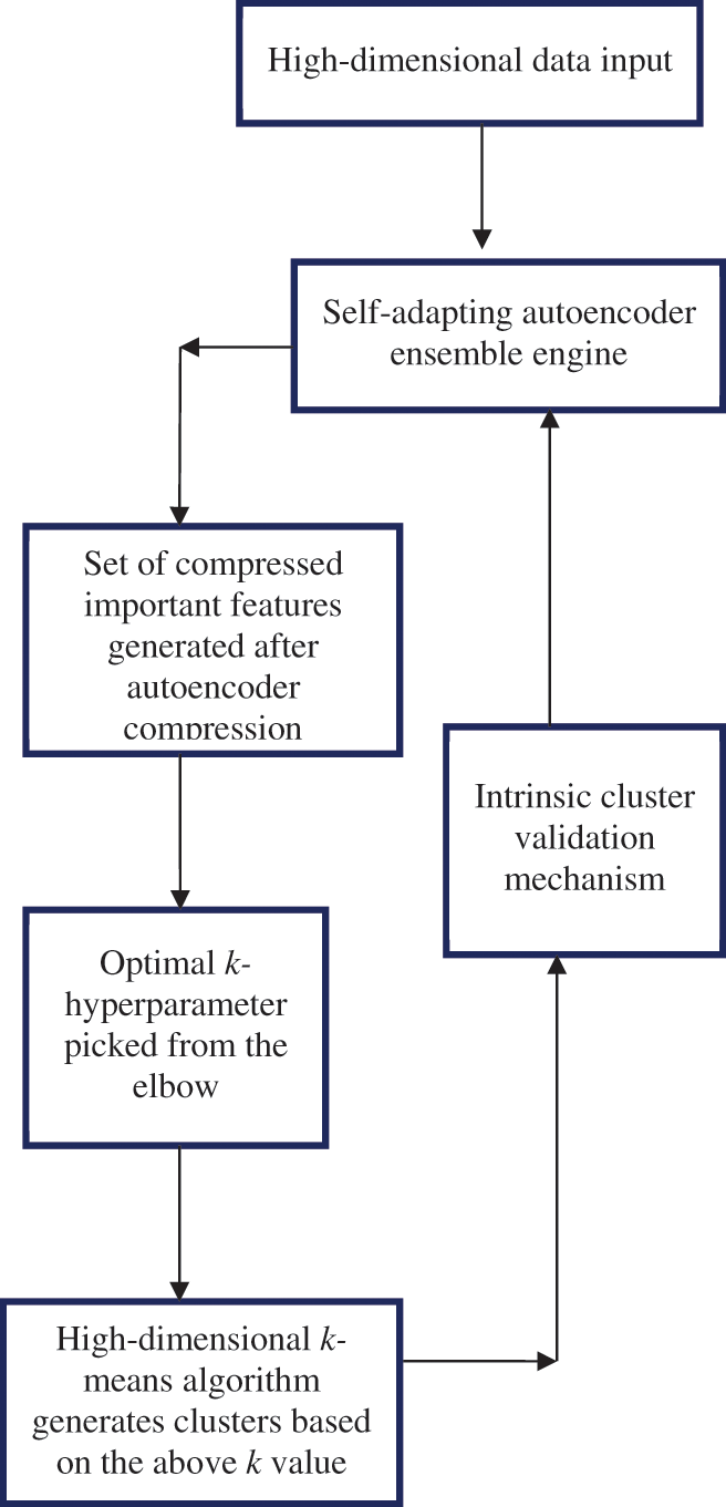
Figure 5: Ensemble based k-hyperparameter optimization technique on a smooth elbow using a self-adapting autoencoder and internal validation index

The following pseudo code represents the functionality of the newly developed k-hyperparameter tuning technique on a smooth elbow in high-dimensional space clustering:

1. KHT ← [HD] # Input high-dimensional dataset into the technique

2. A ← [E] # Initialize autoencoder ensemble

3. HDNature ← HD #Check for the nature of the high-dimensional dataset

4. If HD = = Text of dimensionality X then

5. A ← [K*,HSTX] #Activate the best set of hyperparameter settings for text of X dimensions (K)

6. Else if

7. If HD = = Image of dimensionality X then

8. A ← [K*,HSIX] #Activate the best set of hyperparameter settings for image of X dimensions (K)

9. Else if

10. If HD = = Audio of dimensionality X then

11. A ← [K*,HSAX] # Activate the best set of hyperparameter settings for Audio of X dimensions (K)

12. Else if

13. If HD = = Videos of dimensionality X then

14. A ← [K*,HSVX] #Activate the best set of hyperparameter settings for Video of X dimensions (K)

15. End if

16. End if

17. End if

18. End if

19. HD ← LD # Map the high-dimensional features into low dimensional

20. C ← [ ] # Initialize the elbow curve as empty

21. C* ← [K-values, inertia] # Generate the elbow curve based on LD

22. If

23. K*←[k1] #optimal k is f‴(k)(1+f′(k)2)−3 f″(k)2f″((k)2f′(k) ≈0 at elbow

24. AND

25. K* ← [k2]optimal k aligning to best scores of the validation indexes

26. AND

27. K* ← [k3] optimal k aligning to autoencoder’s latent space visualization

28. Then

29. CI,DI,DB,SI ← [ ] #Initialize all internal validation indexes as empty

30. [Clusters] ← K-means(HD,K*) # Do k-means clustering based on K*

31. [SI, CI,DBn,DI] ← Clusters # Compute internal index scores for clusters

32. If SI,CI,DBn, DI ≠ SI*,CI*,DBn*,DI* # Check if the index scores are best

33. Then

34. Go to step 5

35. Else

36. EI [SI, CI,DBn,DI] ← EI # Compute the ensemble index based on the four internal indexes

37. End

4  Experimental Results and Discussions

Here, the results of the experiments were analyzed and discussed before reaching the conclusion and making recommendations for future research on the k-hyperparameter tuning problem.

4.1 Elbow Visualization of the GLA-BRA-180 High-Dimensional Dataset before and after Compression by the Self-Adapting Autoencoder Ensemble

The main objective of this experiment was to investigate the effect of the autoencoder compression process on the visualization of a high-dimensional dataset using an elbow curve. In Fig. 6, we visualize the GLA-BRA-180 high-dimensional dataset on an elbow, before and after the autoencoder compression process. Before the autoencoder compression process, experimental results show that the elbow curve is smooth and ambiguous, making it difficult to identify a clear elbow. On the other hand, there is evidence of improved visualization of the elbow curve after compressing the high-dimensional dataset with the autoencoder. This compression generated an approximately accurate k-hyperparameter value of 4, compared to the visualization of the original uncompressed data. This demonstrates the ability of the self-adapting autoencoder ensemble to forcefully compress low-level representations of deeply correlated data points from a high-dimensional space, and generate distinct clusters with low intra-cluster variations in an unsupervised manner.

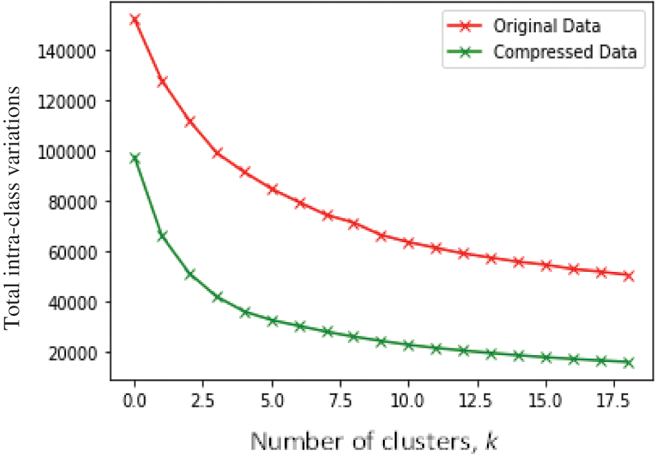
Figure 6: Visualization of the elbow on GLA-BRA-180 dataset before and after autoencoder compression

4.2 Total Intra-Cluster Variations on the GLA-BRA-180 Dataset before and after the Autoencoder Compression

In Fig. 7, we compare the intra-cluster variations of the GLA-BRA-180 high-dimensional dataset before and after the autoencoder encoding process. Intra-cluster variation is a concept in clustering that states that objects within the same cluster should have minimal distances. The results indicate that the total intra-cluster variations on the GLA-BRA-180 dataset are relatively higher between k = 1 and k = 5 before the autoencoder compression process, compared to the total intra-cluster variations after the autoencoder compression process for the same k values. This demonstrates the importance of the autoencoder compression process in reducing intra-cluster variations and, consequently, improving the k-hyperparameter tuning processes and the quality of clustering results, as stated by [115].

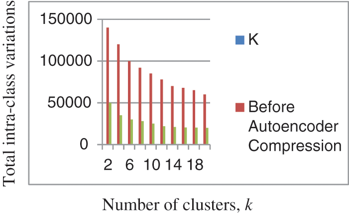
Figure 7: Comparison of the intra-cluster variations on GLA-BRA-180 dataset before and after autoencoder compression

4.3 Cochran’s Q Score Test for Determining if There Is a Statistically Significant Difference in the Optimal K Values Generated across the Different K-Hyperparameter Tuning Techniques on GLA-BRA-180 Dataset

Computed using the R software, the calculated critical Q value has been identified as greater than the critical chi-squared value. For this reason, the null hypothesis has been rejected, and the alternative hypothesis has been retained. We therefore conclude that there is a statistically significant difference in the optimal k-hyperparameter values generated by the ensemble-based technique using a self-adapting autoencoder and internal validation index, compared to the k-hyperparameter values generated by other k-hyperparameter optimization techniques.

4.4 MC Nemar’s Test for Determining if There Is a Statistically Significant Difference in the K-Hyperparameter Value before and after the Autoencoder Compression Process on the GLA-BRA-180 Dataset

The MC Nemar’s score of 19.25, which is greater than the value of 4.6178, provides strong evidence to retain the alternative hypothesis and reject the null hypothesis. Based on this, we can confirm that the compression process of the ensemble-based technique using a self-adapting autoencoder has a significant impact on the k-hyperparameter optimization process for a smooth elbow. Data scientists should therefore adopt this technique as one of the methods for analyzing the high-dimensional datasets that are prevalent in everyday life.

4.5 Comparison of the Identification of the Optimal K-Hyperparameter among the Four Internal Validation Metrics Values on the Self-Adapting Autoencoder Ensemble Based Technique on GLA-BRA-180 Dataset

We further compare the values of the four commonly used internal validation metrics with the ensemble-based k-hyperparameter tuning technique using a self-adapting autoencoder on the GLA-BRA-180 dataset. These four commonly used internal validation metrics include the Davies Bouldin index (DB), Calinski Harabsz index (CH), silhouette index (SI), and Dunn index (DI). A score of one (1) indicates the best performance of the internal validation metric and determines the optimal k-value, while a score of zero (0) indicates that the optimal k-value has not yet been reached. For example, when k =1, the values for all four internal validation metrics are zero because their scores are not the highest. In this case, k = 1 is not considered the optimal value for k on this dataset. This trend is consistent when k = 2, 6, 7, 8, 9, 10, 11, 12, 13, 14, 15, 16, 17, 18, 19, and 20. However, when k = 3, we obtain the Dunn index score that produces the optimal value for the number of clusters, which is three. Moreover, when k = 5, we obtain the Davies Bouldin index, which yields the highest score when the number of clusters is five. Based on the ensemble voting scheme of the autoencoder, the value of k is taken as four. This is because it is the optimal number of clusters at which both the silhouette index and Calinski-Harabasz index produce their highest scores. These results are in Table 1 below.

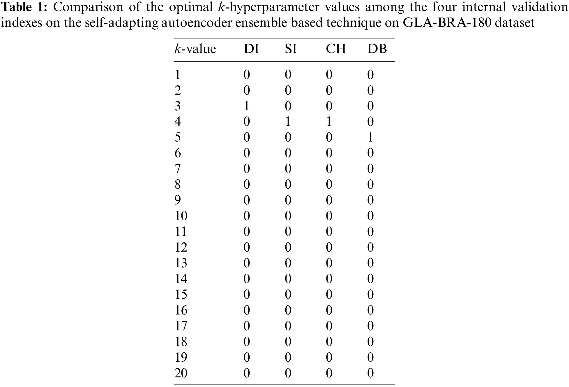
In the table above, the Dunn index and Davies Bouldin index provided inconsistent information regarding the GLA-BRA-180 dataset. Based on the ensemble voting scheme of the proposed technique, the optimal value for the k-hyperparameter is determined to be four (4). This value aligns with the trade-off of the autoencoder’s latent space and the ensemble internal validation index score. Additionally, it generates a value of 0 or close to 0 on the derivative f‴(k)(1+f′(k)2)−3 f″(k)2f″((k)2f′(k) at the elbow. Table 2 below presents a comparison of the performance of the new technique against existing ones on various high-dimensional datasets.

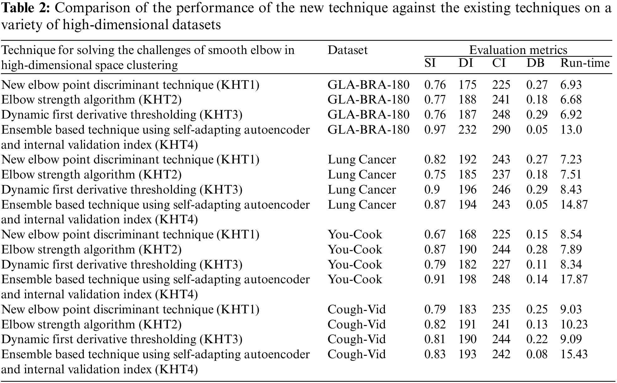
Based on the table above, we conducted an ANOVA analysis to examine the significant differences between the existing techniques and the newly developed technique used to address the challenges of smooth elbow in high-dimensional space clustering. This ANOVA analysis was conducted on the silhouette index, Dunn index, Calinski-Harabasz index, Davies-Bouldin index, and runtime scores. In the first three internal validation indexes, higher values indicate better clustering. In the Davies-Bouldin index, higher values indicate poorer clustering, while lower values indicate better clustering. Higher run times, on the other hand, indicate a lower quality clustering technique. For this reason, we have used DB_N to represent the Davies Bouldin index scores and Time_N to represent the runtime scores. This standardization allows for consistent interpretation of the results across all evaluation metrics. Both standardization and normalization were applied to these variables. The normalization process was performed to standardize the scale without distorting the differences in the values. On the other hand, the standardization process was done in order to ensure that the variables contribute equally to the data analysis process. The following formulas were used for standardization and normalization, respectively.

Xnormalized=(X−Xmin)/(Xmax−Xmin)(21)

Xstandardized=(X−Mean)/Standard deviation(22)

In the following tables (Tables 3–11), we conducted ANOVA analysis on the Silhouette index, Dunn index, Calinski Harabsz index, Davies Bouldin index, and run times. Table 3 presents the ANOVA analysis of the Silhouette index for different techniques used to address the challenges of smooth elbow detection on various high-dimensional datasets. Table 5 presents the ANOVA analysis of the Dunn index for the various techniques employed to address the smooth elbow challenges on a range of high-dimensional datasets. Table 7 presents the ANOVA analysis of the Calinski Harabsz index for the various techniques employed to address the smooth elbow challenges on a range of high-dimensional datasets. Table 9 presents the ANOVA analysis of the Davies Bouldin index for the various techniques employed to address the smooth elbow challenges on a range of high-dimensional datasets. Table 11 presents the ANOVA analysis of the run times for various techniques used to solve the smooth elbow challenges on a range of high-dimensional datasets.

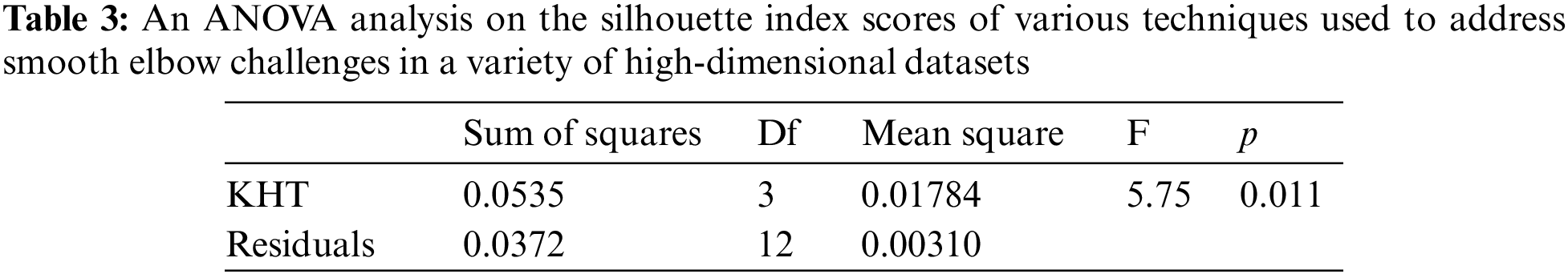
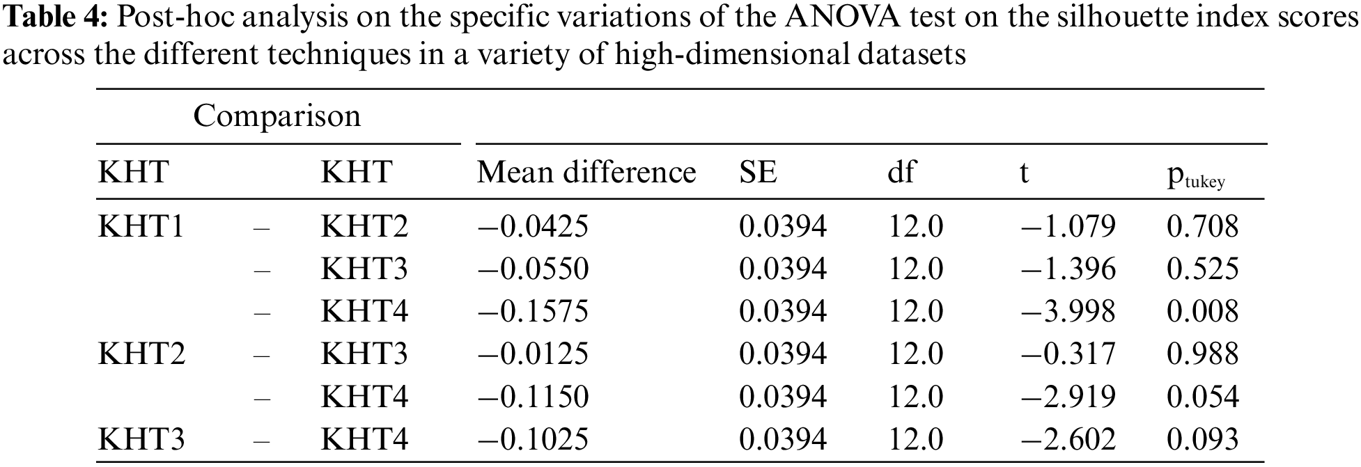
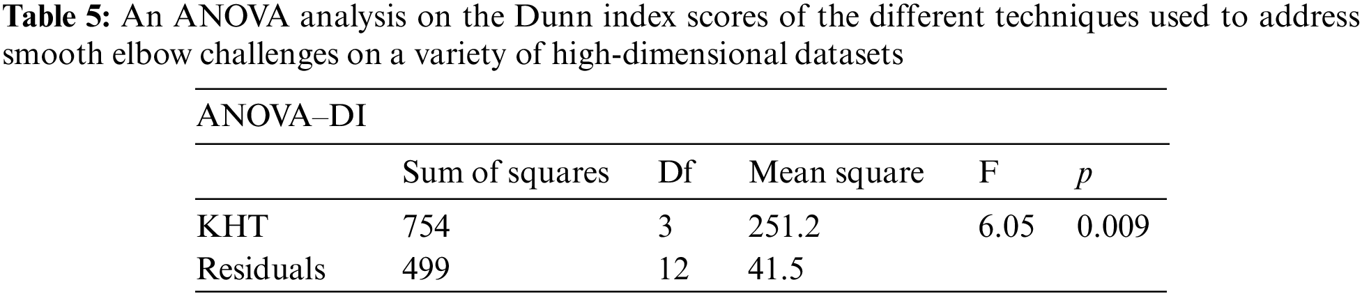
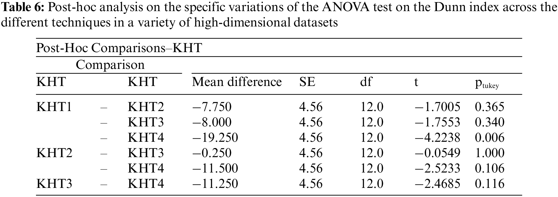
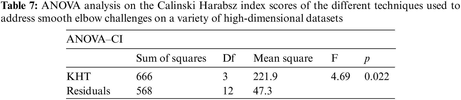
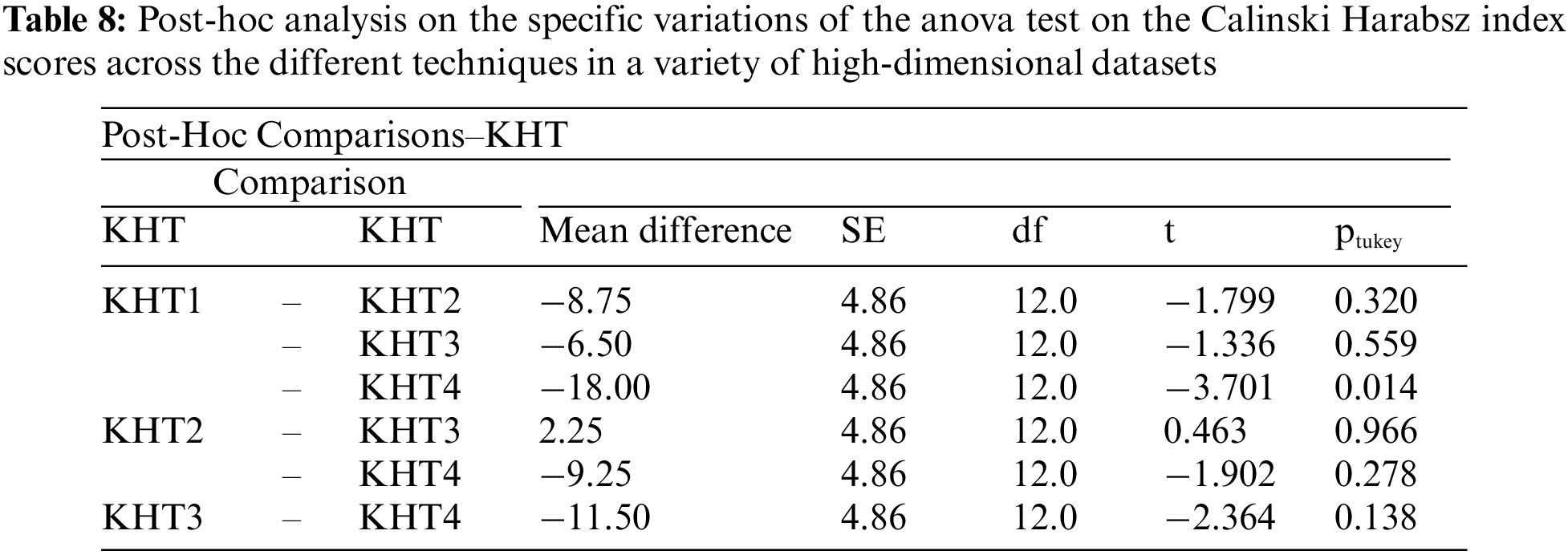
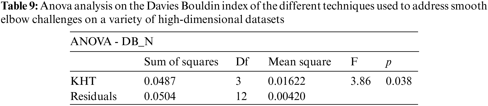
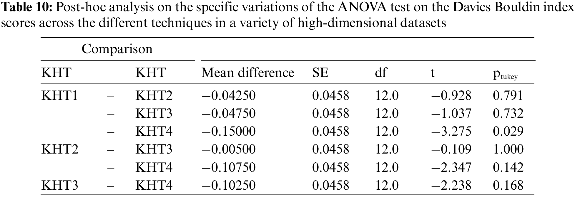
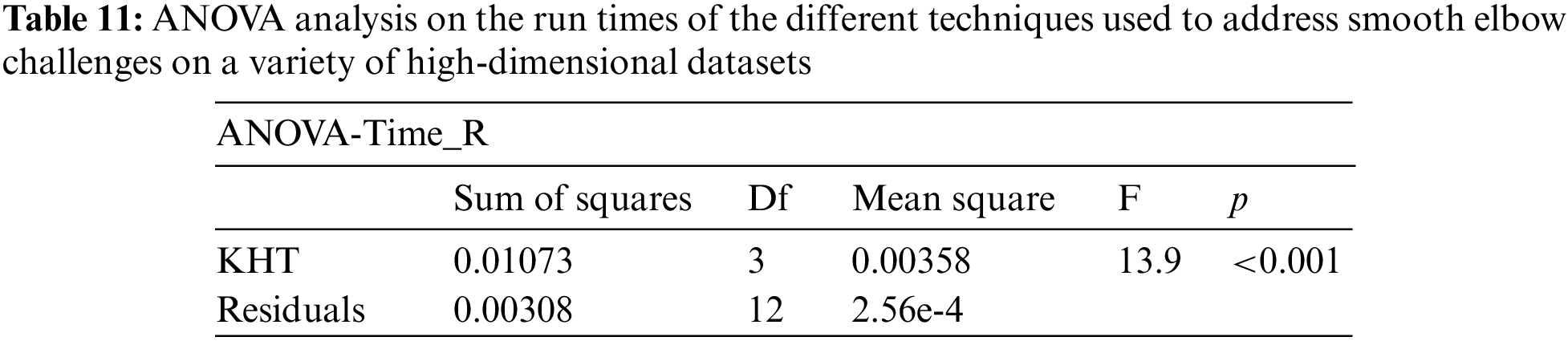
The low p-value of 0.011 indicates that there is a statistically significant variation among the different k-hyperparameter tuning techniques. Based on this evidence, we conducted further post-hoc analysis to investigate the specific differences of the ANOVA test on the Silhouette index scores using different k-hyperparameter tuning techniques. These posthoc results are included in Table 4.

From the above table, it is evident that the significant effect of the different k-hyperparameter tuning techniques was driven by the differences between techniques KHT1 and KHT4 (the new technique). There was mainly no statistically significant difference in the performance of the other techniques.

The low p-value of 0.009 indicates that there is a statistically significant variation among the different k-hyperparameter tuning techniques. Based on this evidence, we conducted further post-hoc analysis to investigate the specific differences of the ANOVA test on the Dunn index scores for the different k-hyperparameter tuning techniques. These post-hoc results are included in Table 6.

From the above table, it is evident that the significant effect of the different k-hyperparameter tuning techniques was driven by the differences between techniques KHT1 and KHT4 (the new technique). There was mainly no statistically significant difference in the performance of the other techniques.

The low p-value of 0.022 indicates that there is a statistically significant variation among the different k-hyperparameter tuning techniques. Based on this evidence, we conducted further post-hoc analysis to investigate the specific differences of the ANOVA test on the Calinski Harabsz index scores for the different k-hyperparameter tuning techniques. These post-hoc results are included in Table 8.

From the above table, it is evident that the significant effect of the different k-hyperparameter tuning techniques was driven by the differences between techniques KHT1 and KHT4 (new technique) only. There was, mainly, no statistical significant difference in the performance of the other techniques.

The low p-value of 0.038 indicates that there is a statistically significant variation among the different k-hyperparameter tuning techniques. Based on this evidence, we conducted further post-hoc analysis to investigate the specific differences of the ANOVA test on the Davies Bouldin index scores using different k-hyperparameter tuning techniques. These post-hoc results are included in Table 10.

The low p-value of less than 0.01 indicates that the observed difference is unlikely to have occurred by chance alone. This supports the conclusion that there are significant variations in run times across the different k-hyperparameter tuning techniques. Based on this evidence, we conducted further post-hoc analysis to investigate the specific differences of the ANOVA test on the run time scores of the different k-hyperparameter tuning techniques. These post-hoc results are included in Table 12.

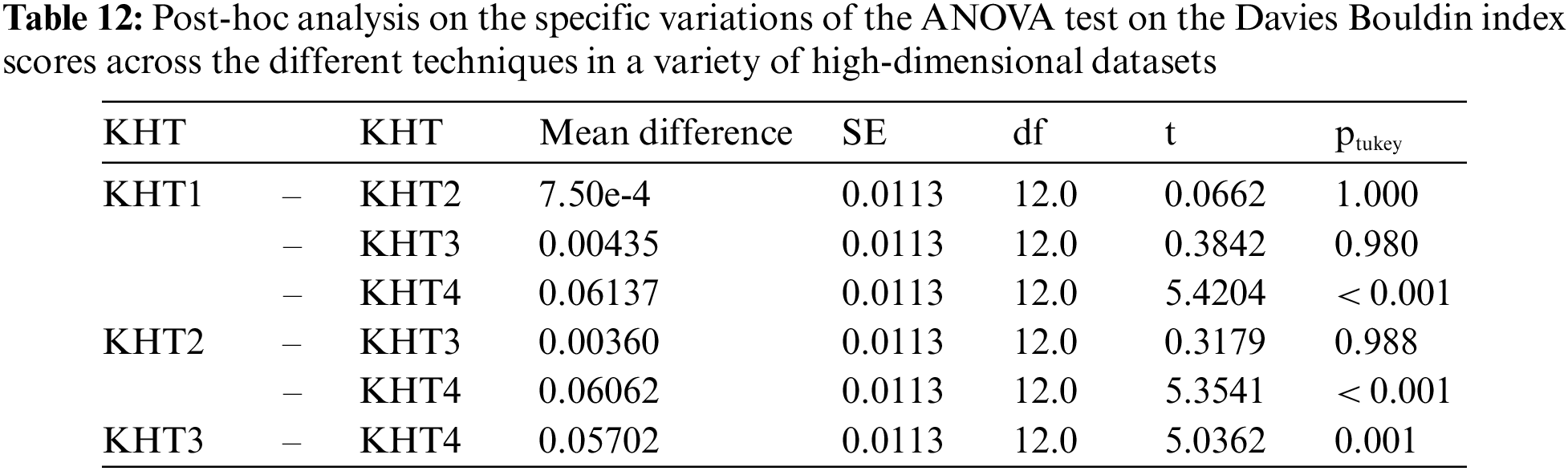
From the above table, it is evident that the significant effect of the different k-hyperparameter tuning techniques was driven by the differences between techniques KHT1 and KHT4 (the new technique), KHT3 and KHT4, as well as between techniques KHT2 and KHT4. This demonstrates that there are clear-cut differences in the run times between technique KHT4 and the other techniques. Although the scores of the internal validation indexes for the new technique are relatively good across all four high-dimensional datasets, the run time, on the other hand, is relatively higher. This is a challenge for the newly developed technique.

5  Conclusions and Recommendations

This research has reviewed the existing k-hyperparameter tuning techniques used to address the challenges of smooth elbows in high-dimensional space clustering. The research gaps identified during the review process served as the foundation for developing the new technique. During the evaluation process, both the existing techniques and the new one were validated using a similar set of high-dimensional input datasets and evaluation metrics. The experimental results, based on the ANOVA, Cochran’s Q test, and McNemar’s score, indicate a significant difference in the performance of the ensemble-based self-adapting autoencoder in the k-hyperparameter tuning process compared to other techniques. Specifically, the results show a clearer elbow. The relatively low total intra-cluster variations on the GLA-BRA-180 dataset after the autoencoder compression process demonstrate the importance of the autoencoder compression process in reducing intra-cluster variations. This, in turn, improves the k-hyperparameter tuning process on a high-dimensional dataset. In order to visualize the number of clusters in the latent space, the autoencoder aims to combine the optimal set of hyperparameter settings based on the characteristics of the high-dimensional input dataset. The contribution of this research work was the development of a new technique for k-hyperparameter tuning. This technique is based on an ensemble of a self-adapting autoencoder and internal validation indexes in the k-hyperparameter tuning process. This study contributes to the existing literature on the process of k-hyperparameter tuning for clustering in high-dimensional space, specifically focusing on identifying a smooth elbow. We have also been able to prove that various internal validation metrics may not always provide consistent information about the quality of clusters. Different internal metrics yield different k-hyperparameter values at their best scores. This nullifies the use of internal validation indexes as the primary solution for addressing the challenges of determining the optimal elbow point when the elbow method fails. The adoption of the ensemble validation metric in this paper allows its components to equally respond to the diverse conditions found in a specific high-dimensional dataset. This ensemble validation metric is based on the voting scheme of the bagging ensemble technique. Future research should focus on investigating the performance of the self-adapting autoencoder-based ensemble technique with high-dimensional datasets of varying dimensionality and different data dimensionality reduction methods.

Acknowledgement: The authors thank the entire faculty at both the Department of Engineering and Department of Computer Science of Kenyatta University for supporting this research study.

Funding Statement: The authors received no specific funding for this study.

Author Contributions: The authors confirm contribution to the paper as follows: study conception and design: R. Gikera, J. Mwaura, E. Muuro, S. Mambo; analysis and interpretation of results: E. Muuro, R. Gikera, S. Mambo; draft manuscript preparation: R. Gikera. J. Mwaura. All authors reviewed the results and approved the final version of the manuscript.

Availability of Data and Materials: Data used in this study can be accessed via the following links: https://www.kaggle.com/datasets/andrewmvd/covid19-cough-audio-classification for COVID-19 cough audio, https://opendatalab.com/YouCook/download for YouCook dataset, https://www.kaggle.com/datasets/yusufdede/lung-cancer-dataset for Lung Cancer dataset and https://www.ncbi.nlm.nih.gov/sites/GDSbrowser?acc=GDS1962 for GLA-BRA-180 dataset.

Conflicts of Interest: The authors declare that they have no conflicts of interest to report regarding the present study.

References

1. M. Ahmed, R. Seraj and S. M. S. Islam, “The k-means algorithm: A comprehensive survey and performance evaluation,” Electronics, vol. 9, no. 8, pp. 1295, 2020. [Google Scholar]

2. L. D. L. Fuente-Tomas, B. Arranz, G. Safont, P. Sierra, M. Sanchez-Autet et al., “Classification of patients with bipolar disorder using k-means clustering,” PLoS One, vol. 14, no. 1, pp. e0210314, 2019. [Google Scholar]

3. P. Arora and S. Varshney, “Analysis of k-means and k-medoids algorithm for big data,” Procedia Computer Science, vol. 78, pp. 507–512, 2016. [Google Scholar]

4. H. Ismkhan, “I-k-means−+: An iterative clustering algorithm based on an enhanced version of the k-means,” Pattern Recognition, vol. 79, pp. 402–413, 2018. [Google Scholar]

5. I. W. Septiani, A. C. Fauzan and M. M. Huda, “Implementation of k-medoids algorithm with Davies-Bouldin-index evaluation for clustering postoperative life expectancy in patients with lung cancer,” Journal of Computer Systems and Informatics, vol. 3, pp. 556–566, 2022. [Google Scholar]

6. P. I. D. P. Manivannan and P. I. Devi, “Dengue fever prediction using K-means clustering algorithm,” in 2017 IEEE Int. Conf. on Intelligent Techniques in Control, Optimization and Signal Processing (INCOS), Krishnankoil, India, pp. 1–5, 2017. https://doi.org/10.1504/IJENM.2019.103161 [Google Scholar] [CrossRef]

7. L. A. Serna, K. A. Hernández and P. N. González, “A k-means clustering algorithm: Using the chi-square as a distance,” in Int. Conf. on Human Centered Computing, Mérida, Mexico, pp. 464–470, 2019. [Google Scholar]

8. C. Shi, B. Wei, S. Wei, W. Wang, H. Liu et al., “A quantitative discriminant method of elbow point for the optimal number of clusters in clustering algorithm,” EURASIP Journal on Wireless Communications and Networking, vol. 1, pp. 1–16, 2021. [Google Scholar]

9. A. K. Dubey, U. Gupta and S. Jain, “Analysis of k-means clustering approach on the breast cancer Wisconsin dataset,” International Journal of Computer Assisted Radiology and Surgery, vol. 11, pp. 2033–2047, 2016. [Google Scholar] [PubMed]

10. P. Fränti and S. Sieranoja, “How much can k-means be improved by using better initialization and repeats?,” Pattern Recognition, vol. 93, pp. 95–112, 2019. [Google Scholar]

11. S. K. Majhi and S. Biswal, “Optimal cluster analysis using hybrid K-means and ant lion optimizer,” Karbala International Journal of Modern Science, vol. 4, pp. 347–360, 2018. [Google Scholar]

12. J. Nayak, B. Naik and H. S. Behera, “Cluster analysis using firefly-based K-means algorithm: A combined approach,” in Computational Intelligence in Data Mining. Singapore: Springer, pp. 55–64, 2017. [Google Scholar]

13. I. F. Ashari, E. D. Nugroho, R. Baraku, I. N. Yanda and R. Liwardana, “Analysis of Elbow, Silhouette, Davies-Bouldin, Calinski-Harabasz, and rand-index evaluation on K-means algorithm for classifying flood-affected areas in Jakarta,” Journal of Applied Informatics and Computing, vol. 7, pp. 95–103, 2023. [Google Scholar]

14. J. Blömer, C. Lammersen, M. Schmidt and C. Sohler, “Theoretical analysis of the k-means algorithm-A survey,” in Algorithm Engineering. Cham: Springer, pp. 81–116, 2016. [Google Scholar]

15. A. Punhani, N. Faujdar, K. K. Mishra and M. Subramanian, “Binning-based silhouette approach to find the optimal cluster using K-means,” IEEE Access, vol. 10, pp. 115025–115032, 2022. [Google Scholar]

16. R. W. Grant, J. McCloskey, M. Hatfield, C. Uratsu, J. DRalston et al., “Use of latent class analysis and k-means clustering to identify complex patient profiles,” JAMA Network Open, vol. 3, no. 12, pp. e2029068, 2020. [Google Scholar] [PubMed]

17. J. Qi, Y. Yu, L. Wang and J. Liu, “K-means: An effective and efficient K-means clustering algorithm,” in 2016 IEEE Int. Conf. on Big Data and Cloud Computing (BDCloudSocial Computing and Networking (SocialComSustainable Computing and Communications (SustainCom)(BDCloud-SocialCom-SustainCom), Atlanta, Georgia, USA, pp. 242–249, 2016. https://doi.org/10.1109/BDCloud-SocialCom-SustainCom.2016.46 [Google Scholar] [CrossRef]

18. K. P. Sinaga and M. S. Yang, “Unsupervised K-means clustering algorithm,” IEEE Access, vol. 8, pp. 80716–80727, 2020. [Google Scholar]

19. R. Jothi, S. K.Mohanty and A. Ojha, “DK-means: A deterministic k-means clustering algorithm for gene expression analysis,” Pattern Analysis and Applications, vol. 22, no. 2, pp. 649–667, 2019. [Google Scholar]

20. Z. Karaca, “The cluster analysis in the manufacturing industry with k-means method: An application for Turkey,” Eurasian Journal of Economics and Finance, vol. 6, no. 3, pp. 1–12, 2018. [Google Scholar]

21. B. M. Devassy and S. George, “Dimensionality reduction and visualisation of hyperspectral ink data using t-SNE,” Forensic Science International, vol. 311, pp. 110194, 2020. [Google Scholar]

22. S. Kant and I. A. Ansari, “An improved K means clustering with Atkinson index to classify liver patient dataset,” International Journal of System Assurance Engineering and Management, vol. 7, no. 1, pp. 222–228, 2016. [Google Scholar]

23. I. A. Pagnuco, J. I. Pastore, G. Absras, M. Brun and V. L. Ballarin, “Analysis of genetic association using hierarchical clustering and cluster validation indices,” Genomics, vol. 109, pp. 438–445, 2017. [Google Scholar] [PubMed]

24. J. Xiao, J. Lu and X. Li, “Davies Bouldin Index based hierarchical initialization K-means,” Intelligent Data Analysis, vol. 21, no. 6, pp. 1327–1338, 2017. [Google Scholar]

25. W. L. Zhao, C. H. Deng and C. W. Ngo, “k-means: A revisit,” Neurocomputing, vol. 291, pp. 195–206, 2018. [Google Scholar]

26. X. Ran, X. Zhou, M. Lei, W. Tepsan and W. Deng, “A novel k-means clustering algorithm with a noise algorithm for capturing urban hotspots,” Applied Sciences, vol. 11, no. 23, pp. 11202, 2021. [Google Scholar]

27. M. Zubair, A. Iqbal, A. Shil, E. Haque, M. M. Hoque et al., “An efficient k-means clustering algorithm for analysing COVID-19,” in Int. Conf. on Hybrid Intelligent Systems, Cham, Springer, pp. 422–432, 2021. [Google Scholar]

28. I. Meniailov, K. Bazilevych, K. Fedulov and S. Goranina, “Using the K-means method for diagnosing cancer stage using the Pandas library,” CEUR Workshop Proceedings, vol. 2386, no. 9, pp. 15, 2019. [Google Scholar]

29. S. Dasgupta, “How fast is k-means?,” in Learning Theory and Kernel Machines. Berlin, Heidelberg: Springer, pp. 735, 2003. [Google Scholar]

30. M. Wistuba, N. Schilling and L. Schmidt-Thieme, “Learning hyperparameter optimization initializations,” in 2015 IEEE Int. Conf. on Data Science and Advanced Analytics (DSAA), Paris, France, pp. 1–10, 2015. [Google Scholar]

31. T. Gupta and S. P. Panda, “Clustering validation of CLARA and k-means using silhouette & DUNN measures on Iris dataset,” in 2019 Int. Conf. on Machine Learning, Big Data, Cloud and Parallel Computing (COMITCon), Faridabad, India, pp. 10–13, 2019. https://doi.org/10.1109/COMITCon.2019.8862199 [Google Scholar] [CrossRef]

32. S. S. Yu, S. W. Chu, C. M. Wang, Y. K. Chan and T. C. Chang, “Two improved k-means algorithms,” Applied Soft Computing, vol. 68, pp. 747–755, 2018. [Google Scholar]

33. Š. Brodinová, P. Filzmoser, T. Ortner, C. Breiteneder and M. Rohm, “Robust and sparse k-means clustering for high-dimensional data,” Advances in Data Analysis and Classification, vol. 13, no. 4, pp. 905–932, 2019. [Google Scholar]

34. N. Keriven, N. Tremblay, Y. Traonmilin and R. Gribonval, “Compressive K-means,” in 2017 IEEE Int. Conf. on Acoustics, Speech and Signal Processing (ICASSP), Toronto, Ontario, Canada, pp. 6369–6373, 2017. [Google Scholar]

35. E. Schubert, “Stop using the elbow criterion for k-means and how to choose the number of clusters instead,” arXiv preprint arXiv: 2212.12189, 2022. [Google Scholar]

36. M. K. Islam, M. S. Ali, M. S. Miah, M. M. Rahman and M. S. Alam, “Brain tumor detection in MR image using superpixels, principal component analysis and template based K-means clustering algorithm,” Machine Learning with Applications, vol. 5, pp. 100044, 2021. [Google Scholar]

37. C. Yuan and H. Yang, “Research on K-value selection method of K-means clustering algorithm,” J, vol. 2, no. 2, pp. 226–235, 2019. [Google Scholar]

38. A. Asai, M. Konno, M. Taniguchi, A. Vecchione and H. Ishii, “Computational healthcare: Present and future perspectives,” Experimental and Therapeutic Medicine, vol. 22, no. 6, pp. 1–13, 2021. [Google Scholar]

39. N. Nidheesh, K. A. Nazeer and P. M. Ameer, “An enhanced deterministic K-means clustering algorithm for cancer subtype prediction from gene expression data,” Computers in Biology and Medaicine, vol. 91, pp. 213–221, 2017. [Google Scholar] [PubMed]

40. M. J. Wainwright, “Sparse linear models in high dimensions,” in High-Dimensional Statistics: A Non-Asymptotic Viewpoint. Cambridge, England: Cambridge University Press, pp. 194–208, 2019. [Google Scholar]

41. C. Giraud, “Introduction,” in High-Dimensional Statistics. London, New York: Chapman and Hall/CRC Press, pp. 3–17, 2021. [Google Scholar]

42. J. H. Wang and C. T. Yang, “Identification of gene-environment interactions by non-parametric kendall’s partial correlation with application to TCGA ultrahigh-dimensional survival genomic data,” Frontiers in Bioscience (Landmark Ed), vol. 27, no. 8, pp. 225, 2022. [Google Scholar]

43. K. R. Moon, D. V. Dijk, Z. Wang, S. Gigante and D. B. Burkhardt, “Visualizing structure and transitions in high-dimensional biological data,” Nature Biotechnology, vol. 37, no. 12, pp. 1482–1492, 2019. [Google Scholar] [PubMed]

44. M. Liao, Y. Li, F. Kianifard, E. Obi and S. Arcona, “Cluster analysis and its application to healthcare claims data: A study of end-stage renal disease patients who initiated hemodialysis,” BMC Nephrology, vol. 17, no. 1, pp. 1–14, 2016. [Google Scholar]

45. D. S. Cho, F. Khalvati, D. A. Clausi and A. Wong, “A machine learning-driven approach to computational physiological modeling of skin cancer,” in Int. Conf. Image Analysis and Recognition, Montreal, QC, Canada, pp. 79–86, 2017. [Google Scholar]

46. C. Gaser, R. Dahnke, P. M. Thompson, F. Kurth and E. Luders, “CAT-a computational anatomy toolbox for the analysis of structural MRI data,” bioRxiv, 2022. https://doi.org/10.1101/2022.06.11.495736 [Google Scholar] [CrossRef]

47. M. Zhao, Y. Tang, H. Kim and K. Hasegawa, “Machine learning with k-means dimensional reduction for predicting survival outcomes in patients with breast cancer,” Cancer Informatics, 2018. https://doi.org/10.1177/1176935118810215 [Google Scholar] [PubMed] [CrossRef]

48. R. Singh and E. Rajesh, “Prediction of heart disease by clustering and classification techniques prediction of heart disease by clustering and classification techniques,” International Journal of Computer Sciences and Engineering, vol. 7, no. 5, pp. 861, 2019. [Google Scholar]

49. D. Q. Wei, A. C. Kaushik, G. Selvaraj and Y. Pan, “Computational genomics and molecular medicine for emerging COVID-19,” IEEE/ACM Transactions on Computational Biology and Bioinformatics, vol. 18, no. 4, pp. 1227–1229, 2021. [Google Scholar]

50. C. Ritter, T. Wollmann, P. Bernhard, M. Gunkel and D. M. Braun, “Hyperparameter optimization for image analysis: Application to prostate tissue images and live cell data of virus-infected cells,” International Journal of Computer Assisted Radiology and Surgery, vol. 14, no. 11, pp. 1847–1857, 2019. [Google Scholar] [PubMed]

51. Q. Y. Xie, A. Almudevar, C. L. Whitney-Miller, C. T. Barry and M. N. McCall, “A microRNA biomarker of hepatocellular carcinoma recurrence following liver transplantation accounting for within-patient heterogeneity,” BMC Medical Genomics, vol. 9, no. 1, pp. 1–11, 2016. [Google Scholar]

52. P. Silitonga, “Clustering of patient disease data by using K-means clustering,” International Journal of Computer Science and Information Security, vol. 15, no. 7, pp. 219–221, 2017. [Google Scholar]

53. D. C. Sujatha, D. M. Kumar and M. C. Peter, “Building predictive model for diabetics data using K Means Algorithm,” International Journal of Management, IT and Engineering, vol. 8, no. 7, pp. 58–65, 2018. [Google Scholar]

54. G. A. Robinson, J. Peng, P. Dönnes, L. Coelewij and M. Naja, “Disease-associated and patient-specific immune cell signatures in juvenile-onset systemic lupus erythematosus: Patient stratification using a machine-learning approach,” The Lancet Rheumatology, vol. 2, no. 8, pp. e485–e496, 2020. [Google Scholar] [PubMed]

55. Z. Xie, “Computational medicine,” Current Molecular Medicine, vol. 20, no. 6, pp. 407, 2020. [Google Scholar] [PubMed]

56. P. Sarker, M. M. H. Shuvo, Z. Hossain and S. Hasan, “Segmentation and classification of lung tumor from 3D CT image using K-means clustering algorithm,” in 2017 4th Int. Conf. on Advances in Electrical Engineering (ICAEE), Dhaka, Bangladesh, pp. 731–736, 2017. [Google Scholar]

57. D. L. G. Franco, “Computational anatomy strategies for characterization of brain patterns associated with Alzheimer’s disease,” Doctoral Dissertation, University of Antwerp, Antwerp, Belgium, 2022. [Google Scholar]

58. S. Hyun, P. Kaewprag, C. Cooper, B. Hixon and S. M. Bruce, “Exploration of critical care data by using unsupervised machine learning,” Computer Methods and Programs in Biomedicine, vol. 194, pp. 105507, 2020. [Google Scholar] [PubMed]

59. R. C. de Amorim, “A survey on feature weighting-based k-means algorithms,” Journal of Classification, vol. 33, no. 2, pp. 210–242, 2016. [Google Scholar]

60. P. Zhang, A. Cobat, Y. S. Lee, Y. Wu and C. S. Bayrak, “A computational approach for detecting physiological homogeneity in the midst of genetic heterogeneity,” The American Journal of Human Genetics, vol. 108, no. 6, pp. 1012–1025, 2021. [Google Scholar] [PubMed]

61. D. J. Lehmann and H. Theisel, “Optimal sets of projections of high-dimensional data,” IEEE Transactions on Visualization and Computer Graphics, vol. 22, no. 1, pp. 609–618, 2015. [Google Scholar] [PubMed]

62. D. T. A. Luong and V. Chandola, “A k-means approach to clustering disease progressions,” in 2017 IEEE Int. Conf. on Healthcare Informatics (ICHI), Park City, UT, USA, pp. 268–274, 2017. [Google Scholar]

63. K. Ning, X. Zhao, A. Poetsch, W. H. Chen and J. Yang, “Computational molecular networks and network pharmacology,” BioMed Research International, 2017. https://doi.org/10.1155/2017/7573904 [Google Scholar] [PubMed] [CrossRef]

64. A. Malav, K. Kadam and P. Kamat, “Prediction of heart disease using k-means and artificial neural network as hybrid approach to improve accuracy,” International Journal of Engineering and Technology, vol. 9, no. 4, pp. 3081–3085, 2017. [Google Scholar]

65. H. Mitsumoto, P. L. Nagy, C. Gennings, J. Murphy and H. Andrews, “Phenotypic and molecular analyses of primary lateral sclerosis,” Neurology Genetics, vol. 1, no. 1, pp. 1–7, 2015. [Google Scholar]

66. Y. Wang, Y. Zhao, T. M. Therneau, E. J. Atkinson and A. P. Tafti, “Unsupervised machine learning for the discovery of latent disease clusters and patient subgroups using electronic health records,” Journal of Biomedical Informatics, vol. 102, pp. 103364, 2020. [Google Scholar] [PubMed]

67. S. K. Prabhakar and H. Rajaguru, “PCA and K-means clustering for classification of epilepsy risk levels from EEG signals—A comparitive study between them,” in 2015 Int. Conf. on Intelligent Informatics and Biomedical Sciences (ICIIBMS), Bangkok, Thailand, pp. 83–86, 2015. [Google Scholar]

68. E. Becht, L. McInnes, J. Healy, C. A. Dutertre and I. W. Kwok, “Dimensionality reduction for visualizing single-cell data using UMAP,” Nature Biotechnology, vol. 37, no. 1, pp. 38–44, 2019. [Google Scholar]

69. W. Cai, “A dimension reduction algorithm preserving both global and local clustering structure,” Knowledge-Based Systems, vol. 118, pp. 191–203, 2017. [Google Scholar]

70. R. Aziz, C. K. Verma and N. Srivastava, “Dimension reduction methods for microarray data: A review,” AIMS Bioengineering, vol. 4, no. 2, pp. 179–197, 2017. [Google Scholar]

71. R. Zebari, A. Abdulazeez, D. Zeebaree, D. Zebari and J. Saeed, “A comprehensive review of dimensionality reduction techniques for feature selection and feature extraction,” Journal of Applied Science and Technology Trends, vol. 1, no. 2, pp. 56–70, 2020. [Google Scholar]

72. X. Zhao, F. Nie, S. Wang, J. Guo and P. Xu, “Unsupervised 2D dimensionality reduction with adaptive structure learning,” Neural Computation, vol. 29, no. 5, pp. 1352–1374, 2017. [Google Scholar] [PubMed]

73. S. Sun, J. Zhu, Y. Ma and X. Zhou, “Accuracy, robustness and scalability of dimensionality reduction methods for single-cell RNA-seq analysis,” Genome Biology, vol. 20, no. 1, pp. 1–21, 2019. [Google Scholar]

74. D. Bank, N. Koenigstein and R. Giryes, “Autoencoders,” arXiv preprint arXiv:2003.05991, 2020. [Google Scholar]

75. M. Alkhayrat, M. Aljnidi and K. Aljoumaa, “A comparative dimensionality reduction study in telecom customer segmentation using deep learning and PCA,” Journal of Big Data, vol. 7, no. 1, pp. 1–23, 2020. [Google Scholar]

76. S. Ayesha, M. K. Hanif and R. Talib, “Overview and comparative study of dimensionality reduction techniques for high dimensional data,” Information Fusion, vol. 59, pp. 44–58, 2020. [Google Scholar]

77. A. J. Onumanyi, D. N. Molokomme, S. J. Isaac and A. M. Abu-Mahfouz, “AutoElbow: An automatic elbow detection method for estimating the number of clusters in a dataset,” Applied Sciences, vol. 12, no. 15, pp. 7515, 2022. [Google Scholar]

78. S. B. Salem, S. Naouali and Z. Chtourou, “A fast and effective partitional clustering algorithm for large categorical datasets using a k-means based approach,” Computers & Electrical Engineering, vol. 68, pp. 463–483, 2018. [Google Scholar]

79. P. M. Shakeel, S. Baskar, V. R. Dhulipala and M. M. Jaber, “Cloud based framework for diagnosis of diabetes mellitus using K-means clustering,” Health Information Science and Systems, vol. 6, no. 1, pp. 1–7, 2018. [Google Scholar]

80. S. Liu, D. Maljovec, B. Wang, P. T. Bremer and V. Pascucci, “Visualizing high-dimensional data: Advances in the past decade,” IEEE Transactions on Visualization and Computer Graphics, vol. 23, no. 3, pp. 1249–1268, 2016. [Google Scholar] [PubMed]

81. M. Shutaywi and N. N. Kachouie, “Silhouette analysis for performance evaluation in machine learning with applications to clustering,” Entropy, vol. 23, no. 6, pp. 759, 2021. [Google Scholar] [PubMed]

82. A. R. Mamat, F. S. Mohamed, M. A. Mohamed, N. M. Rawi and M. I. Awang, “Silhouette index for determining optimal k-means clustering on images in different color models,” International Journal of Engineering & Technology, vol. 7, no. 2, pp. 105–109, 2018. [Google Scholar]

83. B. Gerald, “A brief review of independent, dependent and one sample t-test,” International Journal of Applied Mathematics and Theoretical Physics, vol. 4, no. 2, pp. 50–54, 2018. [Google Scholar]

84. R. Kusumaningrum, “An automatic labeling of K-means clusters based on chi-square value,” Journal of Physics: Conference Series, vol. 801, no. 1, pp. 012071, 2017. [Google Scholar]

85. J. Qi, Y. Yu, L. Wang, J. Liu and Y. Wang, “An effective and efficient hierarchical K-means clustering algorithm,” International Journal of Distributed Sensor Networks, vol. 13, no. 8, 2017. https://doi.org/10.1177/1550147717728627 [Google Scholar] [CrossRef]

86. X. Shen, W. Liu, I. Tsang, F. Shen and Q. S. Sun, “Compressed k-means for large-scale clustering,” in Proc. of the AAAI Conf. on Artificial Intelligence, California, USA, pp. 2527–2533, 2017. [Google Scholar]

87. S. Nawrin, M. R. Rahman and S. Akhter, “Exploreing k-means with internal validity indexes for data clustering in traffic management system,” International Journal of Advanced Computer Science and Applications, vol. 8, no. 3, pp. 264–272, 2017. [Google Scholar]

88. B. Abualhaj, G. Weng, M. Ong, A. A. Attarwala, F. Molina et al., “Comparison of five cluster validity indices performance in brain FET-PET image segmentation using k-means,” Medical Physics, vol. 44, no. 1, pp. 209–220, 2017. [Google Scholar] [PubMed]

89. J. Hämäläinen, S. Jauhiainen and T. Kärkkäinen, “Comparison of internal clustering validation indices for prototype-based clustering,” Algorithms, vol. 10, no. 3, pp. 105, 2017. [Google Scholar]

90. S. G. Rao and A. Govardhan, “Investigation of validity metrics for modified K-means clustering algorithm,” i-Manager’s Journal on Computer Science, vol. 3, no. 2, pp. 33, 2015. [Google Scholar]

91. M. Misuraca, M. Spano and S. Balbi, “BMS: An improved dunn index for document clustering validation,” Communications in Statistics-Theory and Methods, vol. 48, no. 20, pp. 5036–5049, 2019. [Google Scholar]

92. K. R. Rao and B. M. Josephine, “Exploring the impact of optimal clusters on cluster purity,” in 2018 3rd Int. Conf. on Communication and Electronics Systems (ICCES), Coimbatore, Tamil Nadu, India, pp. 754–757, 2018. [Google Scholar]

93. M. Hassani and T. Seidl, “Using internal evaluation measures to validate the quality of diverse stream clustering algorithms,” Vietnam Journal of Computer Science, vol. 4, no. 3, pp. 171–183, 2017. [Google Scholar]

94. P. Roy and J. K. Mandal, “Performance evaluation of some clustering indices,” Computational Intelligence in Data Mining, vol. 3, pp. 509–517, 2015. [Google Scholar]

95. D. Tward, X. Li, B. Huo, B. Lee, P. Mitra et al., “3D mapping of serial histology sections with anomalies using a novel robust deformable registration algorithm,” in Int. Workshop on Multimodal Brain Image Analysis, Switzerland AG, pp. 162–173, 2019. [Google Scholar]

96. L. Gao, J. Song, X. Liu, J. Shao, J. Liu et al., “Learning in high-dimensional multimedia data: The state of the art,” Multimedia Systems, vol. 23, no. 3, pp. 303–313, 2017. [Google Scholar]

97. A. Ly, M. Marsman and E. J. Wagenmakers, “Analytic posteriors for Pearson’s correlation coefficient,” Statistica Neerlandica, vol. 72, no. 1, pp. 4–13, 2018. [Google Scholar] [PubMed]

98. J. J. Pambabay-Calero, S. A. Bauz-Olvera, A. B. Nieto-Librero, M. P. Galindo-Villardon and S. Hernandez-Gonzalez, “An alternative to the cochran-(Q) statistic for analysis of heterogeneity in meta-analysis of diagnostic tests based on HJ biplot,” Investigación Operacional, vol. 39, no. 4, pp. 536–545, 2018. [Google Scholar]

99. M. Jain, M. Jain, T. AlSkaif and S. Dev, “Which internal validation indices to use while clustering electric load demand profiles?,” Sustainable Energy, Grids and Networks, vol. 32, pp. 100849, 2022. [Google Scholar]

100. A. Cockburn, P. Dragicevic, L. Besançon and C. Gutwin, “Threats of a replication crisis in empirical computer science,” Communications of the ACM, vol. 63, no. 8, pp. 70–79, 2020. [Google Scholar]

101. H. Xiong and Z. Li, “Clustering validation measures,” in Data Clustering, vol. 23, London, England: Chapman and Hall/CRC, pp. 571, 2018. [Google Scholar]

102. X. Dong, Z. Yu, W. Cao, Y. Shi and Q. Ma, “A survey on ensemble learning,” Frontiers of Computer Science, vol. 14, pp. 241–258, 2020. [Google Scholar]

103. K. S. Khan, R. Kunz, J. Kleijnen and G. Antes, “Five steps to conducting a systematic review,” Journal of the Royal Society of Medicine, vol. 96, no. 3, pp. 118–121, 2003. [Google Scholar] [PubMed]

104. M. Le Mercier, S. Fortin, V. Mathieu, R. Kiss and F. Lefranc, “Galectins and gliomas,” Brain Pathology, vol. 20, no. 1, pp. 17–27, 2010. [Google Scholar] [PubMed]

105. S. Yagcioglu, A. Erdem, E. Erdem and N. Ikizler-Cinbis, “RecipeQA: A challenge dataset for multimodal comprehension of cooking recipes,” arXiv preprint arXiv:1809.00812, 2018. [Google Scholar]

106. N. K. Chowdhury, M. A. Kabir, M. M. Rahman and S. M. S. Islam, “Machine learning for detecting COVID-19 from cough sounds: An ensemble-based MCDM method,” Computers in Biology and Medicine, vol. 145, pp. 105405, 2022. [Google Scholar] [PubMed]

107. P. R. Radhika, R. A. Nair and G. Veena, “A comparative study of lung cancer detection using machine learning algorithms,” in 2019 IEEE Int. Conf. on Electrical, Computer and Communication Technologies (ICECCT), Tamil Nadu, India, pp. 1–4, 2019. [Google Scholar]

108. A. Tashakkori and J. W. Creswell, “Exploring the nature of research questions in mixed methods research,” Journal of Mixed Methods Research, vol. 1, no. 3, pp. 207–211, 2007. [Google Scholar]

109. H. Chouikhi, M. Charrad and N. Ghazzali, “A comparison study of clustering validity indices,” in 2015 Global Summit on Computer & Information Technology (GSCIT), Sousse, Tunisia, pp. 1–4, 2015. [Google Scholar]

110. Y. S. Thakare and S. B. Bagal, “Performance evaluation of K-means clustering algorithm with various distance metrics,” International Journal of Computer Applications, vol. 110, no. 11, pp. 12–16, 2015. [Google Scholar]

111. N. Tomašev and M. Radovanović, “Clustering evaluation in high-dimensional data,” in Unsupervised Learning Algorithms. Cham, German: Springer, pp. 71–107, 2016. [Google Scholar]

112. M. Q. P. Smith and G. D. Ruxton, “Effective use of the McNemar test,” Behavioral Ecology and Sociobiology, vol. 74, no. 11, pp. 1–9, 2020. [Google Scholar]

113. M. Zitnik, F. Nguyen, B. Wang, J. Leskovec, A. Goldenberg et al., “Machine learning for integrating data in biology and medicine: Principles, practice, and opportunities,” Information Fusion, vol. 50, pp. 71–91, 2019. [Google Scholar] [PubMed]

114. S. L. K. Pond, S. D. Frost and S. V. Muse, “HyPhy: Hypothesis testing using phylogenies,” Bioinformatics, vol. 21, no. 5, pp. 676–679, 2005. [Google Scholar] [PubMed]

115. A. Nasser, “Investigating k-means and kernel k-means algorithms with internal validity indices for cluster identification,” Journal of Advances in Mathematics and Computer Science, vol. 30, no. 2, pp. 1–12, 2019. [Google Scholar]