Automatic Driving Operation Strategy of Urban Rail Train Based on Improved DQN Algorithm

1  Introduction

Two components, designing the line running curve and tracking the running curve, make up the traditional automatic train operation control method. This necessitates a precise analysis of the train motion model; however, as the model becomes more accurate, its internal parameters become more complex, resulting in significant challenges in solving these parameters during actual train operations. Consequently, real-time performance cannot be guaranteed. With the rapid development of artificial intelligence, AI technology has shown some advantages in perception, big data processing and decision control in urban traffic, which provides a new way of thinking about the problem of autonomous driving. In recent years, scholars at home and abroad have applied various methods to study the automatic train driving operation strategies. He et al. [1,2] introduced a feedforward control model and designed a nonparametric adaptive iterative learning control algorithm for high-speed trains based on the superior processing capability of iterative learning control algorithms for highly repetitive controlled systems. Yang et al. [3,4] proposed a train speed control algorithm based on self-anti-disturbance control for the train operation speed tracking control problem in complex environment operation, compared with the traditional algorithm and verified the superiority. Zhang et al. [5,6] established an expert system for train control to control trains with neural networks and designed a strategy-based reinforcement learning algorithm to adapt to changing operation scenarios. Wu et al. [7] designed a suitable objective function and developed a train operation strategy to satisfy passenger comfort. Lai et al. [8] designed a platform framework for train comfort scenario simulation based on digital twins to support ATO performance optimization. Zhang et al. [9,10] considered line conditions, developed a train energy saving control model, and investigated energy saving control strategies for urban rail trains using Q-learning algorithms. Su et al. [11,12] used a time planning approach to plan train operation control in terms of train utilization and amount of passenger time, and combined with other conditions to comprehensively evaluated methods to reduce the energy consumption of the subway. In summary, the research of traditional control methods is gradually being optimized and replaced by existing methods, and reinforcement learning has also appeared in the research of train operation control. DQN algorithm in reinforcement learning is able to deal with the autonomous driving problem through the framework of Markov Decision Process (MDP) of reinforcement learning. Through the approximation of deep neural networks and iterative optimization of reinforcement learning, driving strategies can be learned to adapt to different driving environments and task requirements. It is able to extract valuable features from sensory data and improve the performance and robustness of driving decisions through empirical playback and stable learning process, while discrete control facilitates the action planning for automatic train driving. Therefore, this study proposes train driving control based on DQN algorithm and introduces some improvement methods for the shortcomings of traditional DQN algorithm. Additionally, it integrates the specific operational scenarios of train operations, thereby enabling the analysis and implementation of a superior strategy for automatic train driving operations.

2  Train Operation Model and Algorithm Analysis

2.1 Train Model

The analysis of the physical model of the train is one of the main components of the algorithmic environment construction. The train makes a movement and the train state changes after real-time calculations based on this model to get the feedback given by the environment. The train is subjected to complex forces during actual operation, and the single mass point model is a common simplification method, and the train motion conforms to Newton’s laws of mechanics. The forces can be divided into four categories as shown in Fig. 1, and the kinetic equations of the train operation are as follows:

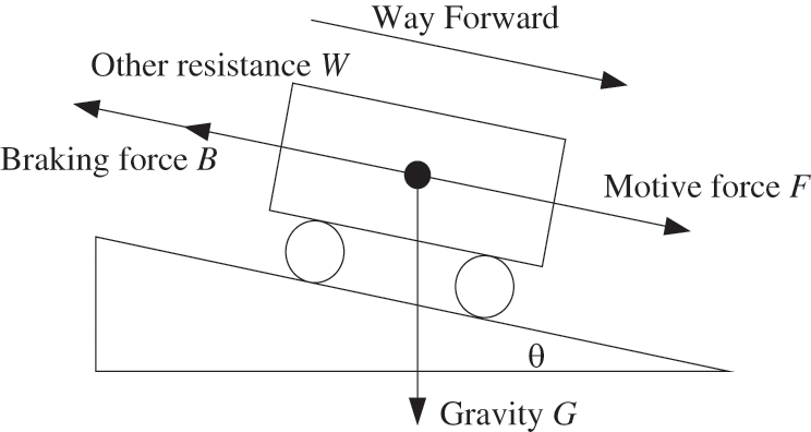
Figure 1: Force diagram of single mass train

{dv(x)dt=F(x)−B(x)−W(x)mdxdt=v(1)

W=(w0+w1)×mg÷1000{w0=a+bv+cv2w1=cr+sin⁡(θ)≈cr+θ(2)

where w0 is the Davis equation, which represents the basic train resistance, where a, b, c are the characteristic parameters determined by the vehicle. w1 is the content of the additional resistance of the line, generally including ramp additional resistance and curve additional resistance, ramp additional resistance is formed by the gravity of the train, expressed by the sine of the slope, generally θ for thousands of grades. In the urban rail line, the line conditions are designed simply and the curve additional resistance is neglected in this study. The units of w0 and w1 for calculating the train resistance are N/kN, which indicates the unit basic resistance.

2.2 Deep Q-Network (DQN) Algorithm

The purpose of deep reinforcement learning is to learn how to control the agent so that the agent makes the appropriate action a based on the current state s, aiming to get as much reward as possible in the future. The classical deep Q-learning method, a value learning approach, combines neural networks with Q-Learning. As in Fig. 2, the neural network structure of DQN is shown.

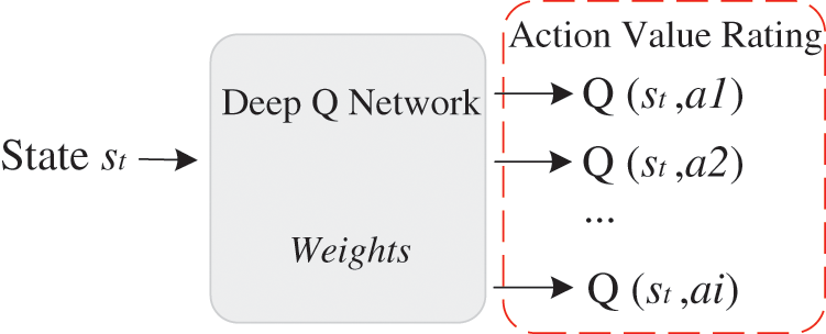
Figure 2: Structure of DQN neural network

The training of DQN adopts Temporal Difference (TD) Learning. TD algorithms are commonly known as Q learning and SARSA, and Q learning algorithm is chosen in this study, and its core idea can be expressed by Eq. (3).

Q(st,at;ω)=rt+γ⋅Q(st+1,at+1;ω)(3)

where rt is the known true reward, and the presence of partially true values makes the method more feasible and logical. ω is the network parameter. γ is the discount factor, which indicates the magnitude of the influence of future rewards on the current action.

The training of DQN can be split into two separate parts, collecting the training data and updating the parameters ω. The more common strategy for selecting actions when collecting training data is generally the ɛ-greedy strategy. The formula is expressed as follows:

at{arg maxaQ(st,a;ω),with the probability (1−ε);Uniform extraction of one actionin A,with the probability ε.(4)

The main procedure of doing gradient descent to update the parameters ω in a DQN network is as follows:

Calculating the TD target,

yt=rt+γ⋅Q(st+1,at+1;ω)=rt+γ⋅maxaQ(st+1,at;ω)(5)

Calculating the loss,

Lt=12[Q(st,at;ω)−yt]2(6)

The gradient descent update parameter,

ωt+1=ωt−α⋅∂L∂ω|ω=ωt(7)

where α is the learning rate parameter, and the value determines the degree of retention of the previous training effect. The parameter ω, after the update is complete, determines the specific value of the amount of traction or braking force that the train will output depending on the current state.

3  Algorithm Improvement and Application

The DQN trained by the original Q-learning algorithm is very unsatisfactory. This article introduces several references to advanced techniques that are highly effective for enhancing DQN. Importantly, these techniques are compatible and can be used in conjunction with one another.

3.1 Over-Estimation

Trains ensure their operation stays safe and stable by selecting appropriate actions. However, if the value of an action is overestimated during the training process, it can compromise the reliability and safety of the action selection. Overestimation is a critical issue that needs to be addressed in train autopilot to ensure a more stable and dependable training process.

The maximization in calculating the TD target causes overestimation of the Q value [13], so the following improvements are made to the DQN algorithm using the Double DQN idea. The assessment of the action is transferred from the initial calculation done by the Q network to the calculation performed by the target network, while the decision-making for selecting the action remains with the Q network. The details are as follows:

{yt=rt+γQt(st+1,at+1;ω−)at+1=arg maxaQ(st+1,a;ω)(8)

ω- and ω are the weight parameters of the target network and Q-network, respectively.

Dueling network [14] makes improvements to the neural network structure of DQN to also alleviate overestimation and increase the stability of the network structure, which is shown in Fig. 3. The basic idea is to decompose the optimal action value Q* into the optimal state value V* plus the optimal advantage D*. The training of the network is the same as that of the deep Q network.

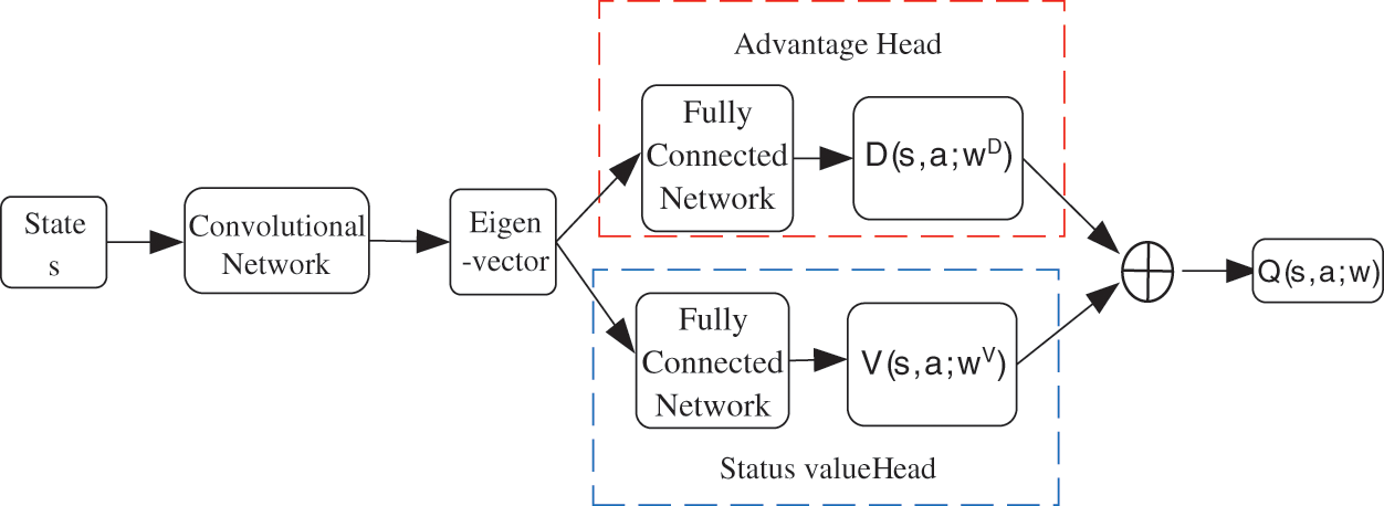
Figure 3: Dueling network structure diagram

The definition of the optimal advantage function is

D∗(s,a)≜Q∗(s,a)−V∗(s).(9)

By mathematical derivation, the optimal action value function Q* is then approximated as the following neural network (duel network).

Q(s,a;w)≜V(s;wV)+D(s,a;wD)−meanaD(s,a;wD)(10)

where wV and wD denote the neural network parameters of the advantage head and status value head, respectively.

3.2 Priority Experience Replay

Not all experience samples in the DQN algorithm contribute equally to the learning process. In train autopilot, experience samples obtained prior to stopping are given high rewards as they are crucial for achieving timely and on-schedule stops. However, if these significant experiences are sparsely sampled, they would be slow to learn. To enhance learning efficiency, optimize strategy with limited experience, and improve algorithm performance, implementing a prioritized experience replay mechanism would be a beneficial choice.

Introducing prioritized experience replay involves departing from the average sampling approach and assigning larger sampling weights to samples with higher learning efficiency [15]. Using the time difference error as a priority indicator, the larger the error, the greater the impact on learning, so priority sampling should be given. This allows for both faster convergence and a higher average return at convergence. Prioritized experience playback gives each experience group a weight, and then non-uniform random sampling is done based on the weights.

The sampling weights (TD error) are defined as

δj≜Q(sj,aj;wnow)−[rt+γ⋅maxaQ(sj+1,a;wnow)](11)

Sampling probability is

pj∝|δj|+l(12)

where l is a very small number that prevents the sampling probability from approaching zero and is used to ensure that all samples are drawn with a non-zero probability.

Due to non-uniform sampling, the sampling probabilities of all samples will be different, which will lead to biased predictions of the DQN, so the learning rate should be adjusted accordingly to offset the bias. Set the learning rate as

αj=α(b⋅pj)β(13)

where b is the total number of samples in the empirical playback array, and β ∈ (0, 1) is a hyperparameter to be tuned. At first β is relatively small and eventually grows to 1.

3.3 Train Operation Model

The mathematical basis and modeling tool for reinforcement learning is Markov decision process (MDP). How to combine the decision process with the actual train operation condition is the key to the design of this algorithm.

3.3.1 Train State Space

At each moment, the environment has a state, the state space is the set of all possible states, noted as S. The train position, speed and running time are defined as the state elements, there are S=[x,v,t]. Here, sk is defined as the state at the end of the kth step, sk={[xk,vk,tk]|xk∈[0,X],vk∈[0,v(xk)lim],tk∈[0,T]}. xk indicates the location of the train at this time, and the interval is the error range from the initial position of the train to the specified stopping position. vk indicates the speed of the train at this time, and the interval is the speed limit from 0 to this position of the train. tk indicates the total running time of the train at this time, and the interval is the error range from the starting time to the specified stopping time of the train.

3.3.2 Train Action Space

The action space during train operation is the set of all possible actions, which is the actual tractive force or braking force output by the train, which is written as A. The urban rail train utilizes a continuous traction mode, wherein the actual tractive force and braking force of the train can be categorized into various levels. The level is 0 in idle state, thus the action selection space corresponds to the number of levels. A k-state action can be represented as follows:

ak=f,(Bmax≤f≤Fmax).(14)

3.3.3 Optimizing the Reward Function

The criteria for a better train operation strategy are generally a combination of safety, on-time performance, energy efficiency, comfort and stopping accuracy. Safety is the responsibility of the train’s ATP system, so reward setting is mainly based on the latter four elements.

Timing bonus. A positive reward is given when a train arrives within the error range of the specified time, and a larger negative reward is given when it is outside the error range. The timing bonus is expressed as Rtime and the formula is expressed as follows:

Rtime={C|T−tn|≤tmin−C|T−tn|>tmin(15)

where C is the reward constant, T indicates the specified running time of the train, and tn indicates the running time of the train at the end of the last state. tmin indicates the error range.

Energy consumption bonus. The actual operating energy consumption magnitude of the train is used as the standard, and the energy consumption within the state transition duration is directly used as the negative reward in each state transition. The energy consumption bonus is expressed in Re, and the formula is expressed as follows:

Re=−μEtn,Exi=|ai×(xi−xi−1)|(16)

where μ is the incentive discount parameter, and the adjustment of this value is a change in the importance given to energy consumption.

The endpoint stopping bonus, with the same design principle as the timing bonus, is expressed as Rstop. The parking error is specified as 0.3 m, K is a constant, and the formula is expressed as follows:

Rstop={K|s−sn|≤0.3−K|s−sn|>0.3(17)

“Comfort” is a very broad and difficult to measure concept [16], narrowly defined as the impact on passengers of vibrations and shocks generated by the train during operation. The speed of change in acceleration, i.e., the magnitude of the impact rate, is a visual representation of the measure of comfort. However, in the DQN algorithm, it is not feasible to use the impact rate as the criterion, for reasons that will be explained in the next sub-section. Therefore, the comfort reward is specified in this study in terms of the magnitude of the actual acceleration, and a negative reward is given when it is greater than a certain measure, and a positive reward is given when it is less than or equal to that measure. At the same time, in order to prevent the sudden change of acceleration from affecting the comfort of passengers, if the acceleration avk+1 after the train state transfer is greater than 0.4 compared with avk before the transfer, a large negative reward is given to the train to ensure the comfort level. Finally, the reward content of “comfort” is expressed by Rs, P and L are constants, and the formula is expressed as follows:

Rs={P+av|av|≤alim−P|av|>alimLavk+1−avk>0.4(18)

In summary, the optimal reward function related to the performance evaluation criteria of automatic train driving during the solution of the operation strategy can then be determined as

Rtrain=Rtime+Re+Rstop+Rs(19)

3.3.4 Other Elements

The fundamental requirement while the train is in operation is to reach the final destination in a safe and stable manner. During the model training process, the selected actions may lead to illogical states such as train reversals, overspeed, or inadequate speed to reach the destination. If the algorithm can incorporate the train’s operational logic and include appropriate constraints, it can help reduce the occurrence of illogical experience arrays. This, in turn, facilitates faster convergence and allows for the training of a more effective operational strategy. Therefore, the following two algorithm settings and improvements are induced:

(1) If the speed of the train at the end of a state is greater than zero, a very small reward value rv is given. This encourages the train to move forward and does not affect the main optimization content, at which point the total reward R can be expressed as

R=Rtrain+Rv.(20)

(2) The restricted speed arrival time tilim is calculated based on the train’s current state si+1. If the train’s remaining running time T−tk is less than tilim, then the action ai made by the train before the state transition must have prevented the train from arriving at the station, resulting in a state that is not in the state space. In order to reduce the number of such empirical arrays, it can be determined that the remaining running time is not enough to return to the action selection to reselect the action. The procedure for calculating the arrival time at the restricted speed is as follows:

a. Obtain the current state sk of the train and get the current running time tk, speed vk and position xk of the train.

b. Accelerate to the limiting speed with the maximum acceleration at the current speed vk and position xk. After that, the train is driven at the restricted speed to the intersection of the acceleration curve and the restricted speed where the train stops with the maximum braking force, and finally stops with the maximum braking force. These three driving states are added together to calculate the restricted speed arrival time tilim. The process is shown in Fig. 4, and the value of t1 + t2 + t3 is the tilim.

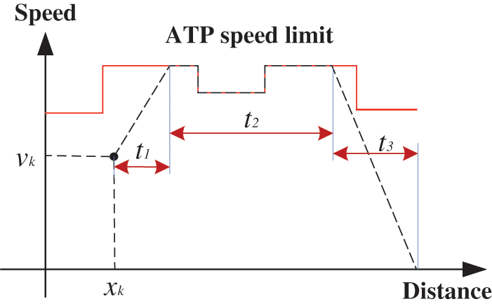
Figure 4: Speed limit arrival time

c. Compare the magnitude of the values of T−tk and tilim. If T−tk < tilim, the train must not arrive at the station on time according to the trip planning, and the action needs to be reselected.

There is a logical flaw in “limiting the speed to the station time” though. The train cannot change its speed suddenly while moving, and the basic resistance of the train is not considered in the calculation. However, the restricted speed of urban rail trains is generally limited to the whole section between stations, and rarely appears in the sub-section speed limit. And this method is introduced mainly to reduce the number of useless empirical arrays and to ensure that trains can arrive at stations within the specified time intervals. Using it for collecting training data is a better improvement of the DQN algorithm to combine with the actual situation of trains. The improved training data collection process is shown in Fig. 5.

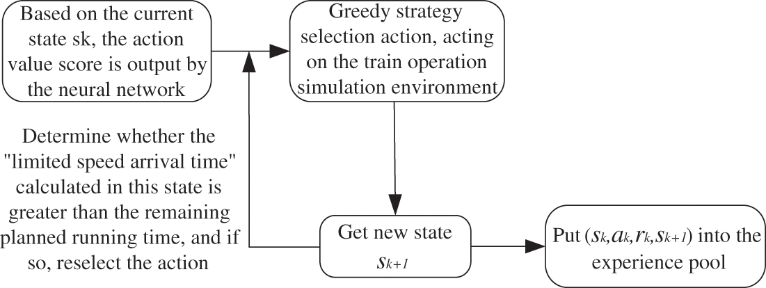
Figure 5: Training data collection process

Regarding the impulse of “comfort”, the output of DQN is not continuous control, but discrete control, and the control force is discrete and constant, so it is not realistic to talk about the derivative of acceleration vs. time. In the ISO2631 standard, the effective value of acceleration is used as an indicator of comfort [17], and the comfort of passengers changes when the acceleration is at different values, as shown in Table 1.

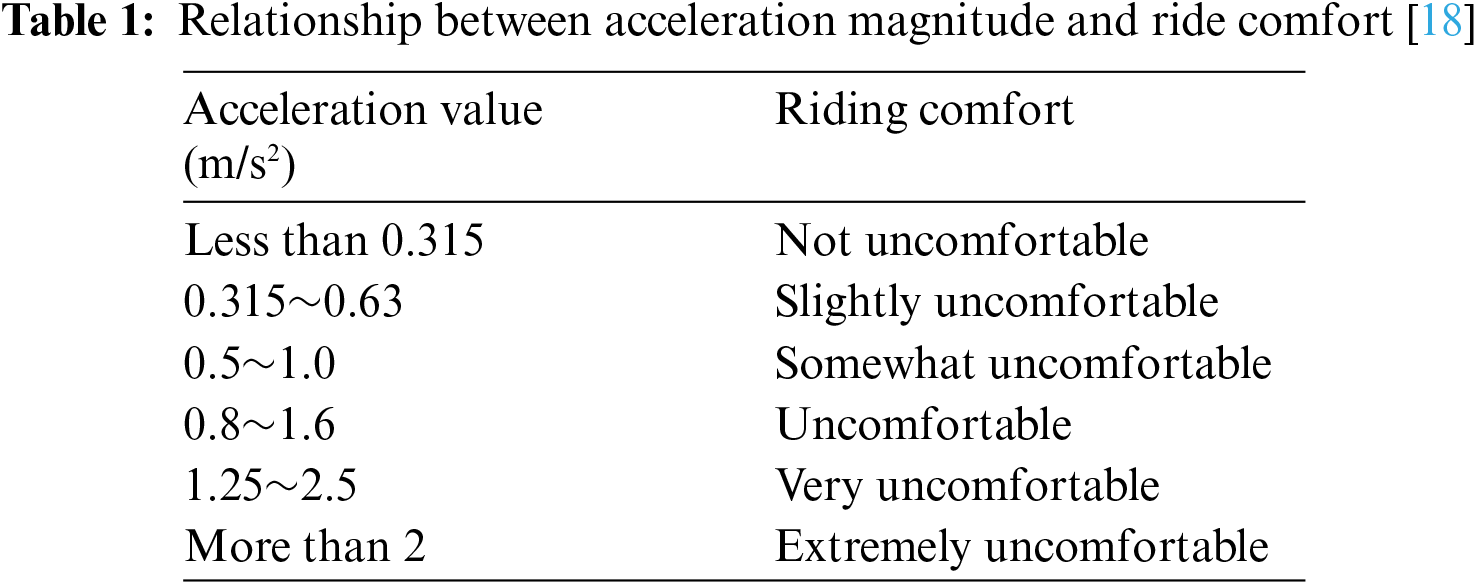
Therefore, the maximum acceleration of the train operation can be controlled by controlling the traction and braking forces to achieve improved passenger ride comfort [19].

3.4 Algorithm Description

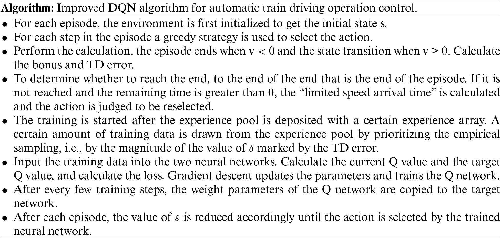
Treating the train as an intelligent body, the train chooses the next action based on the evaluation of the value of the current operating state when it is necessary to change the train’s operating speed. The train position changes and goes to the next state, and the parameters of the neural network are continuously updated by training. The algorithm consists of the construction of the neural network (the train state is a three-dimensional vector and no convolutional layer is needed, so the neural network consists of only fully connected layers), the writing of the train operating environment and the iterative learning code. The complete flow of the algorithm is as follows.

4  Experimental Simulation

4.1 Experimental Platform

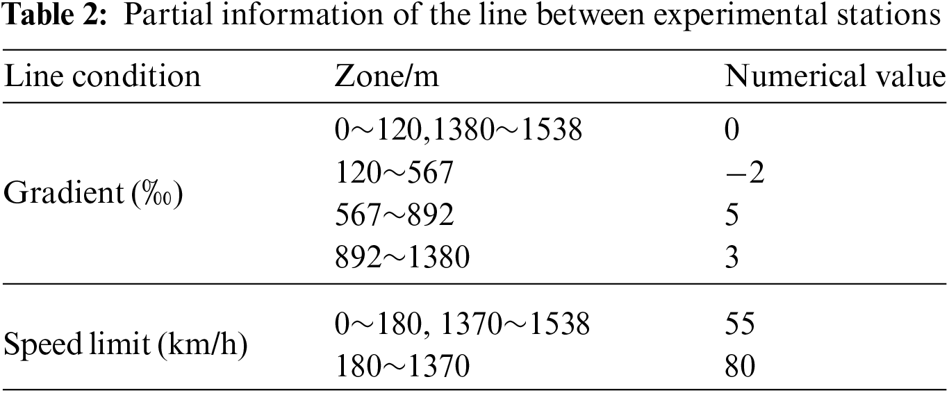
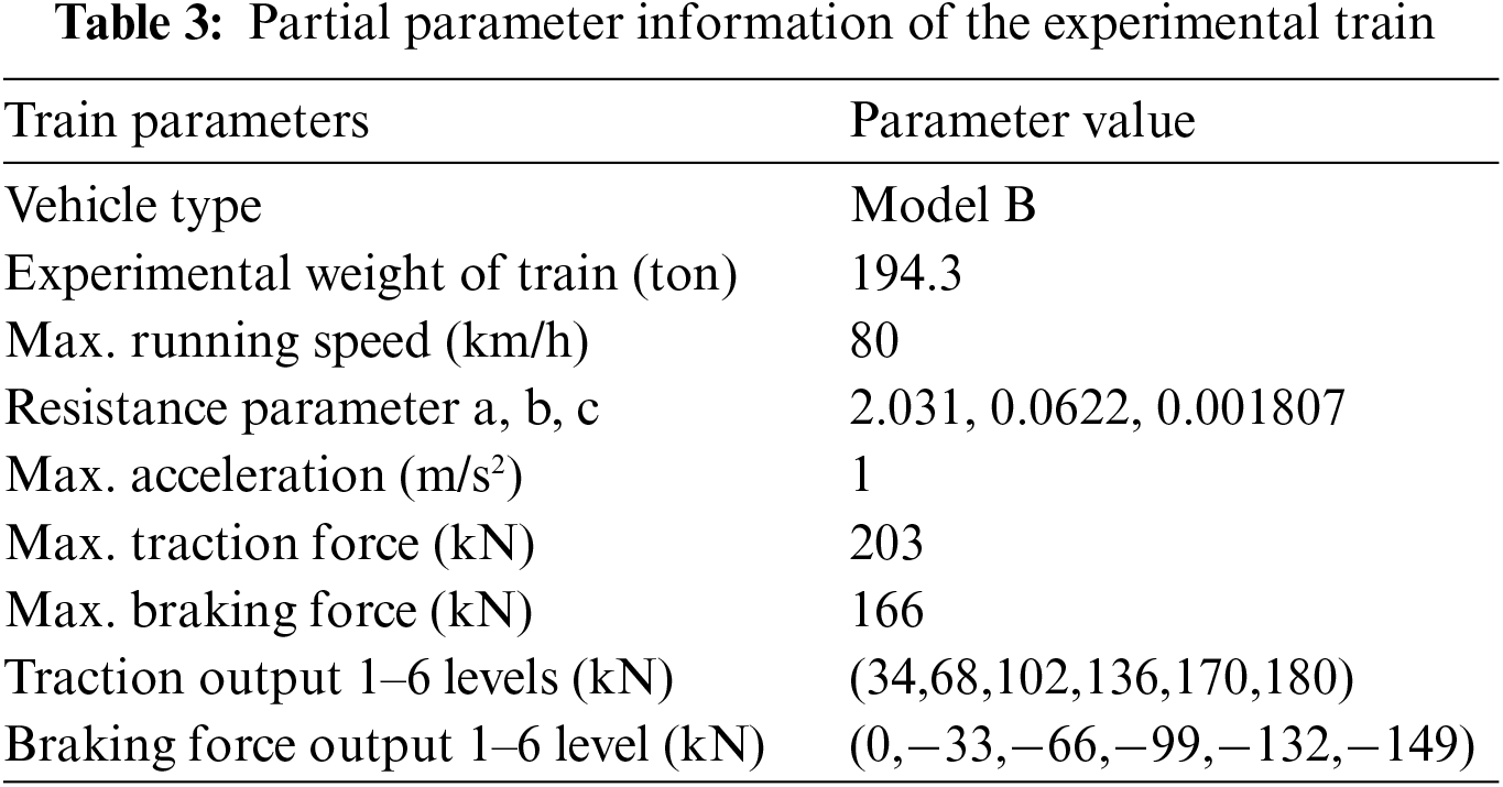
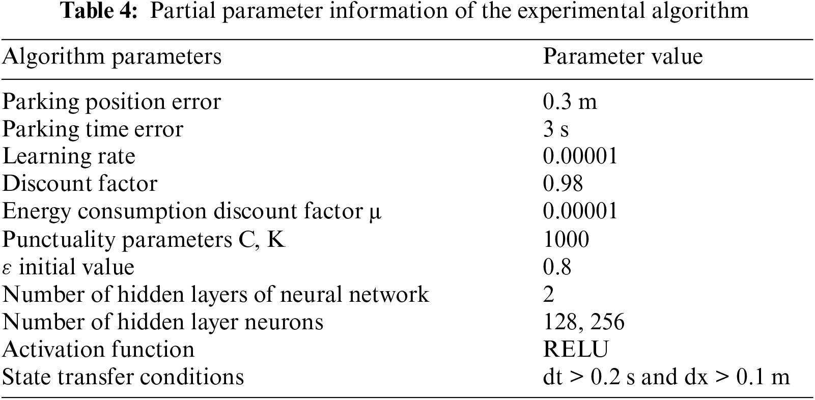
To verify the effectiveness of the improved DQN algorithm proposed in this study for real train operation control, simulations are performed in the PyTorch framework using Python version software. The experiments were conducted on the Beijing Metro Yizhuang Line from Yizhuang Culture Park Station to Wanyuan Street Station. The information of the inter-station line is shown in Table 2. The information of the train part is shown in Table 3. The information of the parameters of the experimental part is shown in Table 4.

4.2 Simulation Results

The algorithm improves on the traditional DQN. As shown in Fig. 6, the reward function curves of the conventional DQN are compared with those of the introduced priority experience playback and dueling networks for the same training scenario at the train running time of 120 s. It can be seen that the latter already converges when the training episodes reach about 800 episodes, while the former starts to converge only when it reaches about 1100 episodes. The efficiency of the algorithm is improved by about 37%. Therefore, the learning ability of the improved algorithm is significantly stronger than that before the improvement.

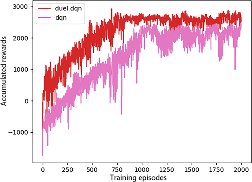
Figure 6: Running 120 s reward curve comparison

As shown in Fig. 7, the reward function curves are compared for the train running time of 130 s. At this time, some parameters of the algorithm are adjusted, the learning rate α is changed from 0.0001 to 0.00001, and the state transfer condition is changed from dt > 0.3 and dx > 0.5 to dt > 0.2 and dx > 0.1. It can be seen that the improved curve starts to converge around 2100 episodes, and the reward value is larger when it converges, and the traditional DQN does not converge. The reasons for this may be that the convergence becomes slower due to the smaller learning rate and the increase in the number of state transfer steps leads to an increase in the reward within episode.

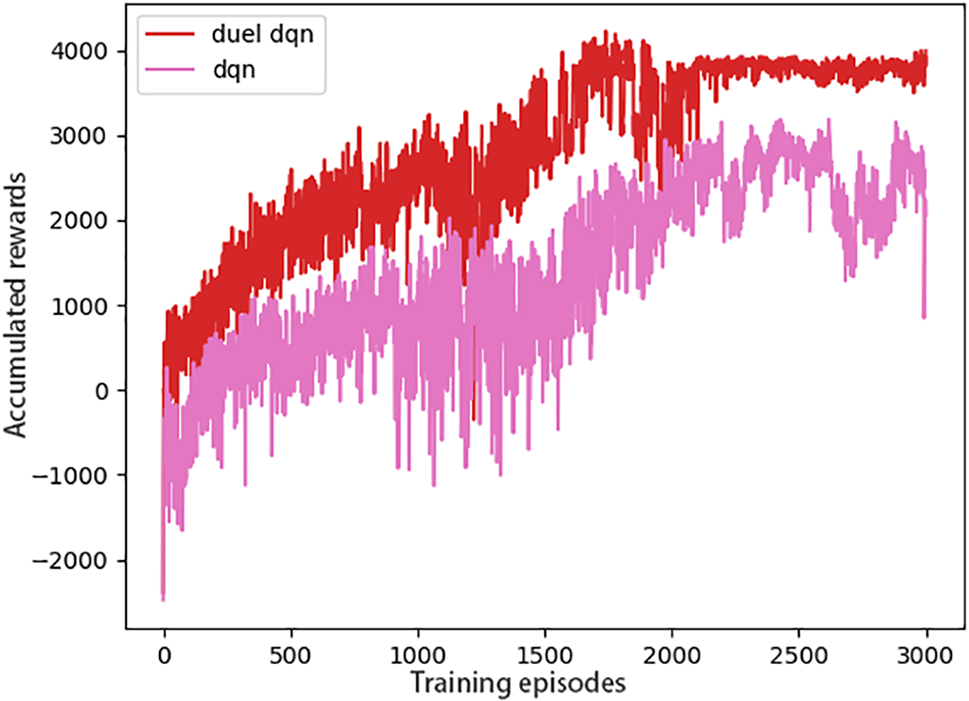
Figure 7: Running 130 s reward curve comparison

In the actual train operation, the train inter-station operation duration and inter-station waiting time are adjusted in real time according to different passenger flow and operation demand. In order to verify the robustness of the algorithm, different inter-station running durations of 120, 130 and 140 s are chosen. 120 s running duration is added to the speed limit section, and the speed limit is 55 km/h at 600–930 m. The speed distance curves and running strategy sequences under four different trip planning are shown in Fig. 8, where the speed unit is m/s.

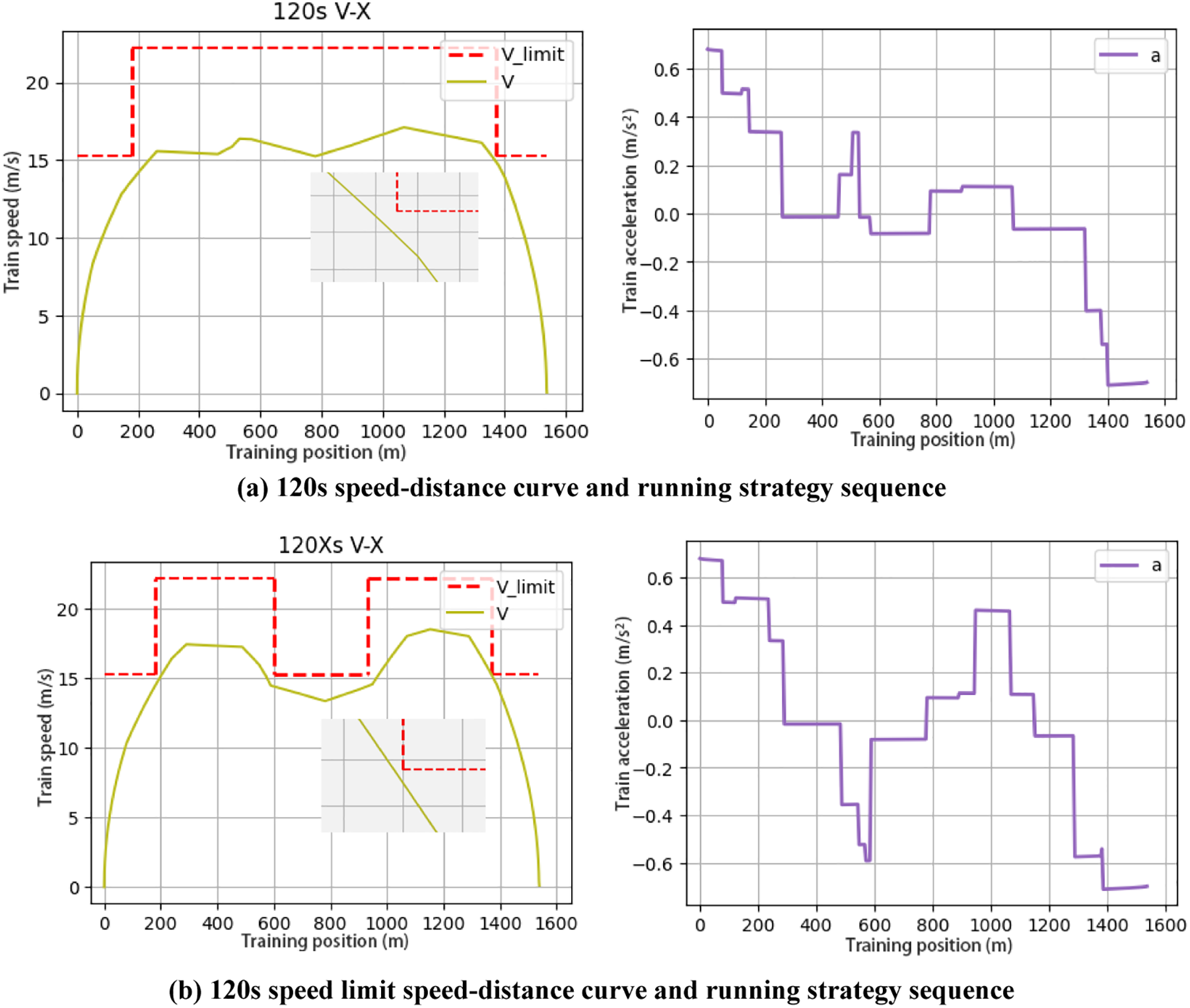
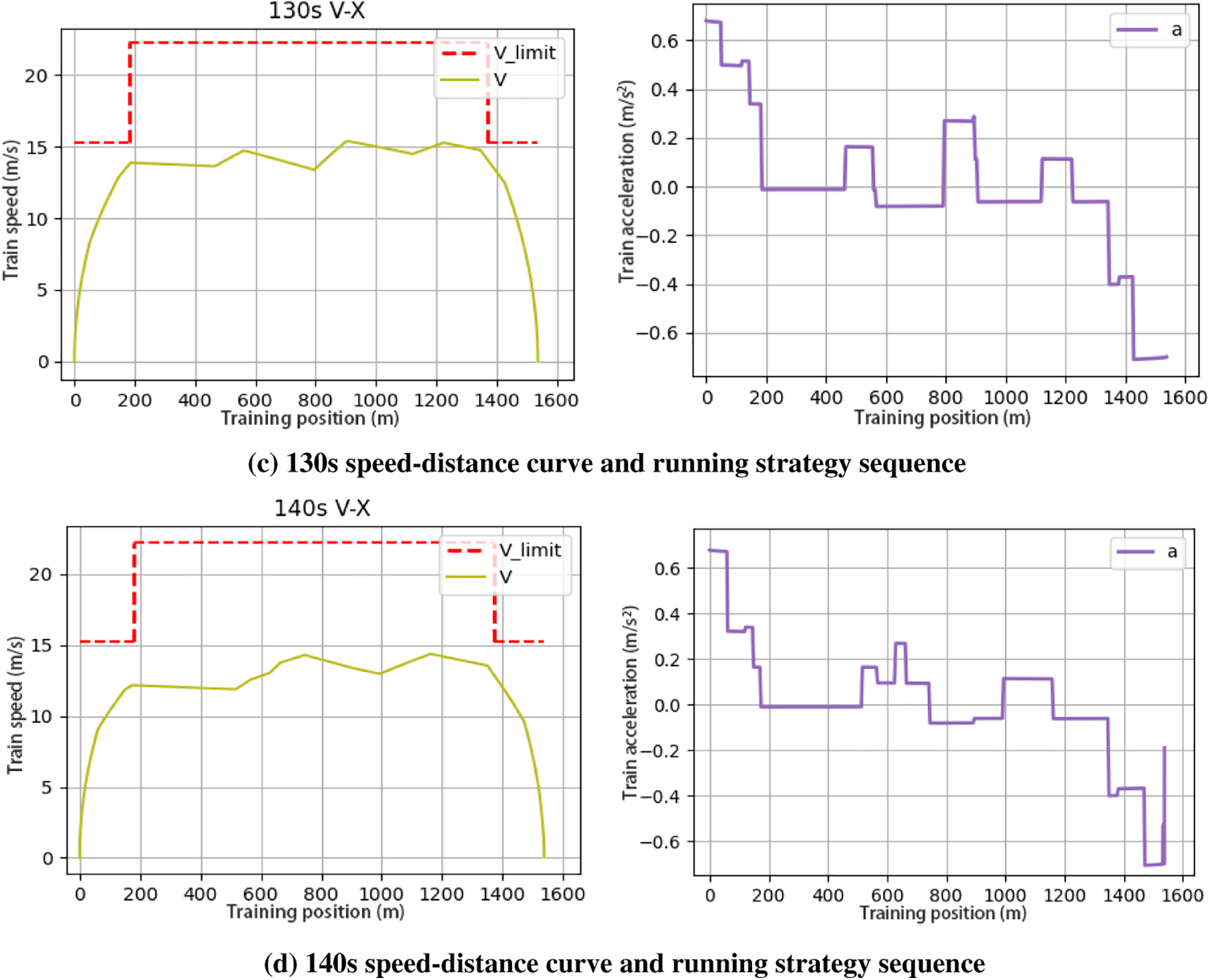
Figure 8: Speed-distance curves and running strategy sequences for different running times

For the four different train operation modes, the algorithm was able to achieve operational results on demand, and its robustness was still good. The train runs without over speeding and meets the ATP protection criteria. Since the control strategy is discrete and constant, it can be seen that there is no cruising process due to the train running resistance, and the whole driving process is controlled by only three ways: traction, idling and braking. This is unavoidable when the DQN method is controlled, but the train operation is in compliance with the standard, and this situation belongs to the characteristics of constant discrete control. From the observation of the control sequence, the train operation meets the requirements of the comfort level specified in the experiment, and the train acceleration does not exceed 0.8, while the change of acceleration during the state transition is not very large. However, there is a change greater than 0.4, which should be due to the control action made by the train in order to stop on time.

In order to more obviously compare the differences between the control situation of this algorithm and the traditional method. Here, the 130 s control curve of the DQN algorithm is directly used as the target curve, and the controller of the PID method is used for tracking. The following tracking curves are obtained, and the control conditions of some sections are intercepted, as shown in Fig. 9.

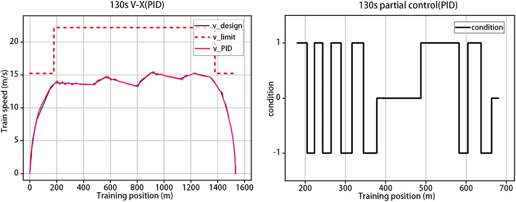
Figure 9: 130 s PID speed-distance curve and some control conditions

From the analysis of the graph, we can observe that the traditional PID control method exhibits noticeable speed tracking errors while controlling the train’s travel. Additionally, there is a certain time delay in adjusting the train’s speed, necessitating frequent changes in the control method to track the curve accurately. This often leads to the scenario depicted on the right side of Fig. 9. Here, 1 represents positive traction, 0 indicates the train is not applying force, and −1 signifies negative traction. During such instances, the train’s speed is high, and within a distance of 500 m, we can see that the train undergoes 13 control condition changes. This frequent switching of conditions within a short period of time places a significant burden on the train’s traction system. It also greatly diminishes passenger comfort. However, with the real-time output control mode employed in this paper, such issues do not arise.

According to the acceleration control sequence, the train travel energy consumption is calculated, and combined with the final state of the train, the train arrival information under the five modes is obtained as shown in the Table 5.

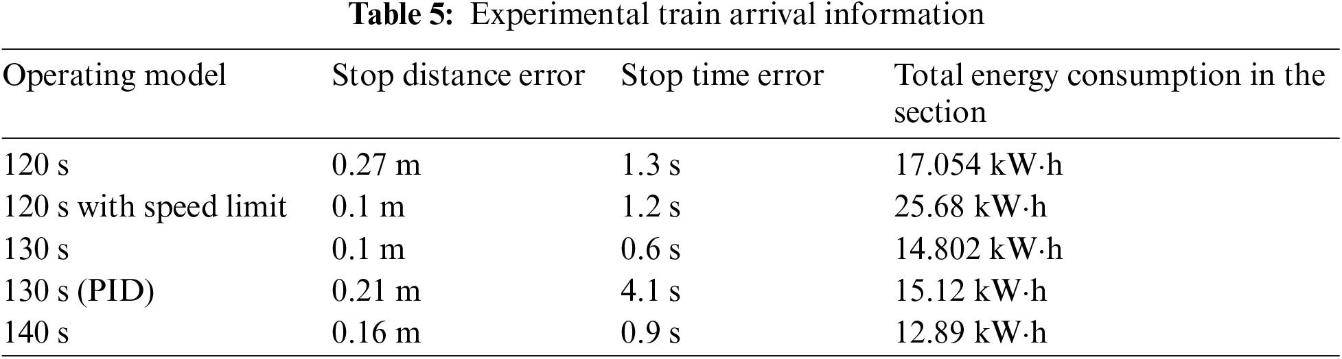
The train stopping data were all in accordance with the design criteria. When the train travels in the selected section, according to the line data statistics, the actual operation of the unoptimized train between stations consumes 15.3 kW·h [20] and the station running time is 144 s. Compared by similar time intervals, the design algorithm in this study consumes 12.89 kW·h at 140 s, which is a good energy saving rate of 15.75%. Compared to 130 s, the energy saving rate is only 3.25%, but the time consumption is reduced by 14.6 s. 120 s consumes more energy due to the shorter operation time, and more energy if the speed limit interval is added. In the PID method, the time error is large due to the more pronounced tracking error. And the energy saving aspect still produces more energy consumption when directly tracking the curve generated by the DQN due to the switching of operating conditions.

According to previous studies, the higher the initial acceleration of the train for the same amount of time, followed by cruising and idling, and the higher the deceleration at stopping, the less energy will be consumed in the train section [5]. In this experiment, since the effect of acceleration magnitude on comfort is considered, the inevitable energy consumption increases compared to what it would be if comfort were not considered.

5  Conclusion

In this study, we have enhanced the traditional DQN algorithm to develop an energy-saving, precise, on-time operation strategy with a certain level of comfort through experimental simulations. This strategy can be applied to various line conditions and operational requirements. The algorithm demonstrates robustness and practicality. In comparison to real-world operations, the experiment shows desirable energy consumption and improved algorithm efficiency.

Currently, the method still allows for potential modifications in the selection of experimental parameters to achieve an optimal parameter configuration. Additionally, due to the discrete action space, there may be deviations in meeting the comfort performance requirements and the optimal utilization and categorization of train traction. In future studies, a continuous control method will be explored, and the reward function will be adjusted accordingly, aiming to discover a more ideal control method for train operation strategy.

Acknowledgement: We would like to express our sincere gratitude to all individuals and institutions involved in this research. Firstly, we would like to thank our supervisor, Professor Bohong Liu, for providing invaluable guidance and support. Your expertise and encouragement have played a vital role in our research. Secondly, we would like to extend our appreciation to all members in Lab 605 at the School of Automation, particularly Ms. Yi Shi. Their technical support and insightful discussions throughout the entire research process have enabled us to overcome challenges and achieve meaningful results. Lastly, we would like to acknowledge all anonymous reviewers and editors for their thorough review and valuable suggestions on our paper. Their comments and guidance have enhanced the quality of our research and propelled us to further refine our methodologies and interpret our findings.

Funding Statement: The authors received no specific funding for this study.

Author Contributions: The authors confirm contribution to the paper as follows: study conception and design: B.H. Liu, T. Lu; data collection: T. Lu; analysis and interpretation of results: T. Lu; draft manuscript preparation: B.H. Liu, T. Lu. All authors reviewed the results and approved the final version of the manuscript.

Availability of Data and Materials: The data that support the findings of this study are available from the corresponding author, B.H. Liu, upon reasonable request.

Conflicts of Interest: The authors declare that they have no conflicts of interest to report regarding the present study.

References

1. Z. Y. He, “Application of adaptive iterative learning control in automatic train driving system,” Ph.D. dissertation, China Academy of Railway Science, China, 2019. [Google Scholar]

2. Z. Y. He and N. Xu, “Non-parametric iterative learning control algorithm for automatic train driving control,” Journal of the China Railway Society, vol. 42, no. 12, pp. 90–96, 2020. https://doi.org/10.3969/j.issn.1001-8360.2020.12.012 [Google Scholar] [CrossRef]

3. J. Yang, Y. Q. Chen and P. P. Wang, “Self-anti-disturbance controller design for train speed tracking based on improved particle swarm algorithm,” Journal of the China Railway Society, vol. 43, no. 7, pp. 40–46, 2021. https://doi.org/10.3969/j.issn.1001-8360.2021.07.006 [Google Scholar] [CrossRef]

4. W. B. Lian, B. H. Liu, W. W. Li, X. Q. Liu, F. Y. Gao et al., “Automatic speed control of high-speed trains based on self-anti-disturbance control,” Journal of the China Railway Society, vol. 42, no. 1, pp. 76–81, 2020. https://doi.org/10.3969/j.issn.1001-8360.2020.01.011 [Google Scholar] [CrossRef]

5. M. Zhang, “Research on automatic train driving method based on reinforcement learning,” Ph.D. dissertation, China Academy of Railway Science, China, 2020. [Google Scholar]

6. M. Zhang, Q. Zhang, W. T. Liu and B. Y. Zhou, “A train intelligent control method based on policy gradient reinforcement learning,” Journal of the China Railway Society, vol. 42, no. 1, pp. 69–75, 2020. https://doi.org/10.3969/j.issn.1001-8360.2020.01.010 [Google Scholar] [CrossRef]

7. J. H. Wu and X. H. Zhang, “Comprehensive evaluation of ride comfort of urban rail trains based on fuzzy reasoning,” Journal of Zhejiang Normal University (Natural Sciences), vol. 40, no. 4, pp. 453–458, 2017. https://doi.org/10.16218/j.issn.1001-5051.2017.04.015 [Google Scholar] [CrossRef]

8. S. H. Lai, C. J. Chen, L. Yan and Y. P. Li, “A comprehensive comfort evaluation system for subway train passengers based on hierarchical analysis,” Science Technology and Engineering, vol. 19, no. 36, pp. 296–301, 2019. [Google Scholar]

9. M. Zhang, Q. Zhang and Z. X. Zhang, “Research on energy-saving optimization of high-speed railroad trains based on Q-learning algorithm,” Railway Transportation and Economy, vol. 41, no. 12, pp. 111–117, 2019. [Google Scholar]

10. Z. L. Jin and X. C. Wu, “Intelligent control strategy for urban rail trains based on Q-learning algorithm,” Railway Standard Design, vol. 66, no. 1, pp. 166–172, 2022. [Google Scholar]

11. S. Su, T. Tang, J. Xun, F. Cao and Y. H. Wang, “Design of running grades for energy-efficient train regulation: A case study for Beijing Yizhuang line,” IEEE Intelligent Transportation Systems Magazine, vol. 13, no. 2, pp. 189–200, 2019. https://doi.org/10.1109/MITS.2019.2907681 [Google Scholar] [CrossRef]

12. R. M. Liu, S. K. Li, L. X. Yang and J. T. Yin, “Energy-efficient subway train scheduling design with time-dependent demand based on an approximate dynamic programming approach,” IEEE Transactions on Systems, Man, and Cybernetics: Systems, vol. 50, no. 7, pp. 2475–2490, 2018. https://doi.org/10.1109/TSMC.2018.2818263 [Google Scholar] [CrossRef]

13. G. C. Gao, “Research on congestion control based on priority empirical replay DQN,” M.S. dissertation, Zhejiang University of Technology and Industry, China, 2022. [Google Scholar]

14. H. Song, Y. B. Liu, J. B. Zhao, J. Y. Liu and G. Wu, “Prioritized replay dueling DDQN based grid-edge control of community energy storage system,” IEEE Transactions on Smart Grid, vol. 12, no. 6, pp. 4950–4961, 2021. https://doi.org/10.1109/TSG.2021.3099133 [Google Scholar] [CrossRef]

15. B. A. Han and J. J. Yang, “Research on adaptive job shop scheduling problems based on dueling double DQN,” IEEE Access, vol. 8, pp. 186474–186495, 2020. https://doi.org/10.1109/ACCESS.2020.3029868 [Google Scholar] [CrossRef]

16. X. X. Zhou, “Optimization analysis of train operation comfort of Tianjin metro line 2,” Electronic World, no. 3, pp. 148–150, 2016. https://doi.org/10.19353/j.cnki.dzsj.2016.03.041 [Google Scholar] [CrossRef]

17. M. Zhao, T. Guo and C. An, “Optimization research of riding comfort of moving train set,” Railway Locomotive & Car, vol. 36, no. 3, pp. 46–50, 2016. https://doi.org/10.3969/j.issn.1008-7842.2016.03.10 [Google Scholar] [CrossRef]

18. J. P. Huang and S. R. Cheng, “Improved particle swarm algorithm for energy-saving control optimization of rail trains,” Journal of East China Jiaotong University, vol. 37, no. 2, pp. 56–63, 2020. https://doi.org/10.16749/j.cnki.jecjtu.2020.02.008 [Google Scholar] [CrossRef]

19. K. Guang, “Research on energy-saving optimization of subway train timing considering ride comfort,” M.S. dissertation, Guangxi University, China, 2021. [Google Scholar]

20. X. T. Chu, “Optimization of energy-saving operation of multi-train urban rail based on ant colony algorithm,” M.S. dissertation, Southwest Jiaotong University, China, 2021. [Google Scholar]