Causality-Driven Common and Label-Specific Features Learning

1  Introduction

Multi-label learning [1] (MLL) is one of the hot research areas in machine learning, which alleviates the problem that instances covering multiple concepts or semantics in numerous real-world application scenarios cannot be accurately handled by traditional single-label algorithms. In real life, MLL has also long been applied in several domains, such as text classification [2], image annotation [3], protein function detection [4] and personalized recommendation [5], to name a few. With the rapid development of the Internet, data is gradually characterized by high dimensional distribution [6]. This can lead to the problem of dimensional catastrophe suffered by multi-label algorithms for data learning.

Label-specific feature (LSF) learning can effectively solve this problem, which is to establish the label-specific relation between labels and features by learning the connection between features and labels. The core idea is that each label should have a specific feature corresponding to it, i.e., the specific features of the label are learned. In multi-label learning, l1-norm can attain feature sparsity and extract label-specific features, which we call private features of labels. The l2,1-norm can also achieve feature sparsity and extract more relevant features of the labels, which we call the common features of the labels.

Label correlation [7] (LC) has long been commonly used in LSF learning, which effectively improves the classification performance of LSF learning algorithms. However, the correlation calculated by cosine similarity is symmetric, and ignore the asymmetric correlation may introduce redundant information in the model. Cosine similarity is also highly susceptible to dimensional catastrophe. As the amount of data increases, the Euclidean distance metric deteriorates. In the process of calculation, the label relevance calculated by cosine similarity is highly susceptible to the a priori knowledge of the labels. Most of the labels in multi-label datasets rely on manual expert marking. With the increase of data volume and the influence of experts’ experience, it is inevitable that there will be omission and miss labeling in the process of marking. For such incomplete datasets, the LC computed by cosine similarity methods are inevitably mixed with many spurious correlations. Therefore, it is necessary to adopt the causal learning [8] algorithm to measure the asymmetric correlation between labels.

In LSF learning, most algorithms only consider the private features of labels and do not consider the common features of labels [9]. However, when we classify two similar labels, the LC of the similar labels are also similarly strongly correlated, but the computed weight matrices are not necessarily similar. As shown in Fig. 1. The labels y1 and y2 are strongly correlated labels, yet the learned weight coefficients are really different. This indicates that we should fully consider the common and private features of labels in the process of classification. Only in this way, the LSF learning can obtain more accurate classification performance.

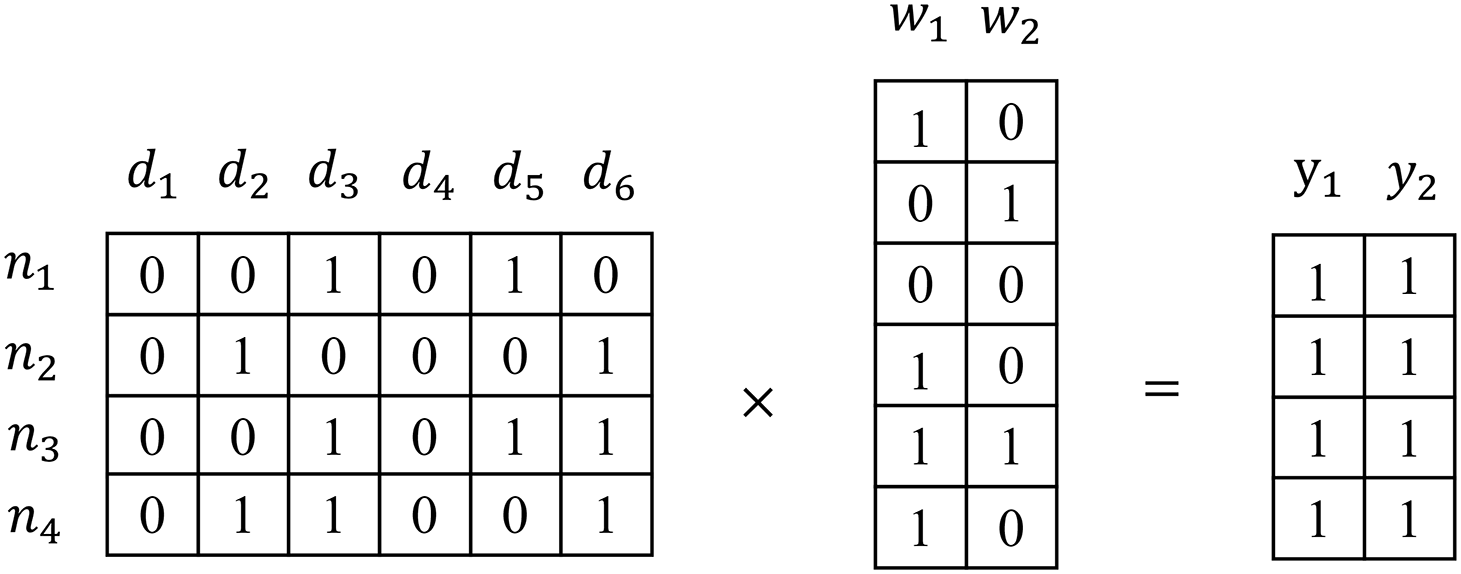
Figure 1: The process of addressing the label-specific feature

Based on the above analysis, we propose a causality-driven common and LSF learning. The main contributions of this paper are as follows:

1) We propose a novel CCSF method, which use l2,1-norm and l1-norm to learn the common and private features of labels, respectively. Thereby, more correlated features are extracted for classification.

2) We use a causal learning algorithm to compute asymmetric label correlations, discarding the traditional way of combining correlation matrix and neighbor matrix, which reduces the influence of original labels.

The remaining sections are organized as follows. Section 2 summarizes some state-of-the-art domestic and international research. The proposed framework and model optimization of CCSF are presented in Section 3. Section 4 analyzes the experimental results and other related experiments. Finally, the conclusion is presented in Section 5.

2  Related Work

Traditional MLL considers that all labels are distinguished based on the same features. However, this categorization is not reasonable and brings a lot of redundant information in the process of categorization, and the classification results are often sub-optimal. Zhang et al. proposed the LSF learning algorithm LIFT [10], which considers that each label is classified based on specific features. Compared with the traditional classification methods, it effectively improves the classification performance of MLL algorithm. But the algorithm does not take into account the correlation between labels. We consider that each label does not exist independently, but has a strong or weak correlation with other labels. The LLSF [11] algorithm proposed by Huang et al. uses the cosine similarity method to measure the correlation between labels. Two strongly correlated labels, whose LSF are also strongly correlated, which further improves the performance of the LSF learning algorithm. By different methods to measure the correlation between labels, Cheng et al. proposed the FF-MLLA [12] algorithm, which utilizes the Minkowski distance to measure the inter-sample similarity based on LC, and uses the singular value decomposition and the limit learning machine to classify multiple labels. The LF-LPLC [13] algorithm proposed by Weng et al. uses the nearest-neighbor technique to consider the local correlation of labels on the basis of the LSF learning algorithm. The algorithm not only enriches the semantic information of labels, but also solves the imbalance problem of labels. The MLFC [14] algorithm proposed by Zhang et al. further improves the performance of the LSF learning algorithm by uniting LSF learning and LC to obtain LSF for each label. For the missing label problem occurring in LSF learning algorithms, the LSML [15] algorithm proposed by Huang et al. utilizes the correlation between labels and has better experimental results not only on the complete dataset, but also on the missing label dataset. Zhao et al. proposed the LSGL [16] algorithm, which considers not only global but also local correlations between labels. LSGL algorithm, based on the assumption that both global and local correlations coexist, has more accurate classification performance than the LSF learning algorithm, which only considers local correlations.

However, most of the above algorithms use cosine similarity to measure out symmetric correlations in the learning of LSF. In fact, the correlation between labels is mostly asymmetric. As the data dimension increases, the Euclidean distance metric becomes less effective. ACML [17] algorithm proposed by Bao et al. and CCSRMC [18] algorithm proposed by Zhang et al. measure the asymmetric correlation between labels using the DC algorithm in causal learning, which are both effective in improving the classification performance of MLL. Luo et al. proposed the MLDL [19] algorithm to fully utilize the structural relationship between features and labels. Not only does it use bi-Laplace regularization to mine the local information of the labels, but it also employs a causal learning algorithm to explore the intrinsic causal relationships between the labels. The BDLS [20] algorithm proposed by Tan et al. introduces a bi-mapping learning framework in LSF learning and uses a causal learning algorithm to calculate the asymmetric correlation between labels, which also effectively improves the classification performance of the LSF learning algorithm. However, the above LSF learning only considers the private features of labels and not the common features of labels. CLML [9] algorithm proposed by Li et al. first uses a norm in the LSF framework to extract the common features of the labels. Subsequently, the GLFS [21] algorithm proposed by Zhang et al. builds a group-preserving optimization framework for feature selection by learning the common features of similar labels and the private features of each label using K-means clustering. Based on the above analysis, we adopt a causal learning algorithm to learn asymmetric LC among labels in LSF learning framework. The l2,1-norm and l1-norm used to extract the common and private features of labels, respectively. The effectiveness of the algorithm in this paper is proved through a large number of experiments.

3  CCSF Model Construction and Optimization

3.1 CCSF Model Construction

In MLL, X denotes the feature matrix, Y represents the label matrix, and the dataset D={(x1,y1),(x2,y2),…,(xn,yn)}, where X∈Rn×d, Y∈Rn×l, l is the number of labels, n is the number of samples, d is the number of features. xn={xn1,xn2,…,xnd} and yn={yn1,yn2,…,ynl} denote the feature and label vectors. The basic model of CCSF in conjunction with the LLSF [10] algorithm proposed by Huang et al. can be written as:

minW12‖XW−Y‖F2+α‖W‖1(1)

where α is the feature sparse parameter, W is the weight coefficient and W=[w1,w2,w3,…,wl]∈Rd×l, and wl∈Rd denotes the LSF of each label. However, Eq. (1) only adopts the l1-norm, which can only extract the private features of the label, but not the shared features of the label. So, we put l2,1-norm in Eq. (1) to extract the common features of labels, and Eq. (2) can be written as:

minW12‖XW−Y‖F2+α‖W‖1+β‖W‖2,1(2)

where β is the feature sparse parameter.

LC has been widely used in LSF learning algorithms, which can effectively improve the classification performance of MLL algorithms. But cosine similarity [22] all calculates symmetric correlations. Indeed, correlations between labels are asymmetric [23]. In this paper, we use a globally structured causal learning algorithm GSBN [24]. First, Markov Blanket (MB) or Parent and Child (PC) part-to-whole structure learning for each label is obtained. Then a directed acyclic graph (DAG) framework is constructed using MB or PC learning.

With the constraint of causal LC, assuming that C is the causal LC matrix and Cij denotes the causal relationship between labels yi and yj. We improve the learning efficiency of LSF by calculating the Euclidean distance between wi and wj, Cij‖wi−wj‖22. When the labels are causally related, the features are similar. Accordingly, wi will be closer to wj. The causal correlation matrix C is defined as follows:

Cij={1yi→yj0yi↛yj(i,j∈1,…,l)(3)

where yi→yj indicates that the label yi is causally related to yj and Cij=1. Conversely yi↛yj indicates that the label yi is not causally related to yj and Cij=0.

Therefore, we add causal constraints based on Eq. (2). The core formula of the CCSF algorithm can be written as:

minW12‖XW−Y‖F2+α‖W‖1+β‖W‖2,1+γtr(WCWT)(4)

where γ is the hyperparameter.

3.2 CCSF Model Optimization

Considering the non-smoothness of the l2,1-norm, we use the technique in the literature [25] to deal with the non-smoothness.

∂‖Wi‖2,1∂Wi=∂Tr(WiTAiWi)∂Wi=2AiWi(5)

where Ai∈Rll is a diagonal matrix with the jth diagonal element Aijj=12‖wij‖2. If wij=0, then Aijj∈∂.

The CCSF model is a convex optimization problem. Due to the non-smoothness of the l1-norm, this paper adopts the accelerated proximal gradient descent method [26] to solve the non-smoothness of the weight matrix W by alternating iterations. The objective function is:

minW∈HF(W)=f(W)+g(W)(6)

where H is the Hilbert space. The expressions for f(W) and g(W) are shown in Eqs. (7) and (8), which are both convex functions and satisfy the Lipschitz condition.

(W)=minW12‖XW−Y‖F2+γtr(WCWT)+β‖W‖2,1(7)

g(W)=α‖W‖1(8)

∇f(W)=XTXW−XTY+2γWC+2AW(9)

For any matrices W1, W2, there is:

‖∇f(W1)−∇f(W2)‖≤Lg‖ΔW‖(10)

where Lg is the Lipschitz constant and ΔW=W1−W2. Introducing the quadratic approximation F(W) for Q(W,W(t)), then

Q(W,W(t))=f(W(t))+(∇f(W(t)),W−W(t))+Lg2‖W−W(t)‖F2+g(W)(11)

Let qt(W)=Wt−1Lg∇f(W), then

W=arg⁡minWQ(W,W(t))=arg⁡minW12‖W−q(t)‖F2+αLg‖W‖1(12)

The optimization algorithm proposed by Lin et al. [27] points out that

W(t)=Wt+θt+1−1θt(Wt−Wt−1)(13)

In Eq. (13), bt satisfies bt+12−bt+1≤bt2. Meanwhile, the convergence rate of O(t−2) is improved, and Wt is the result of the tth iteration. The soft threshold function for performing the iterative operation is shown in Eq. (14).

Wt+1=Sε[q(t)]=arg⁡minWε‖W‖1+12‖W−q(t)‖F2(14)

where Sε[⋅] is the soft threshold operator. For any one parameter xij and ε=αLg, we have

Sε(xij)={xij−εwhen xij>εxij+ε0when xij<−εother(15)

According to f(W), the Lipschitz constant is calculated as:

‖f(W1)−f(W2)‖F2=‖XTXΔW‖F2+‖2γΔWR‖F2+‖2βΔWA‖F2≤2‖XTX‖22‖ΔW‖F2+4γ‖C‖22‖ΔW‖F2+4β‖A‖22‖ΔW‖F2(16)

Therefore, the Lipschitz constant for the CCSF model is:

Lg=2(‖XTX‖22+2γ‖C‖22+2β‖A‖22)(17)

The CCSF algorithm framework is as following:

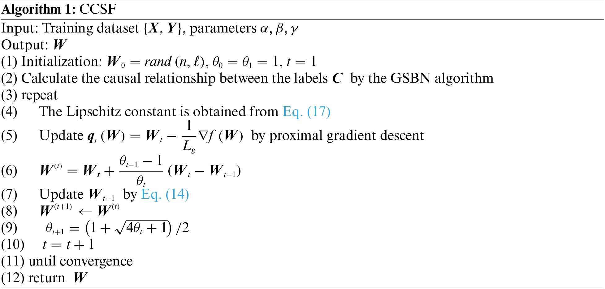
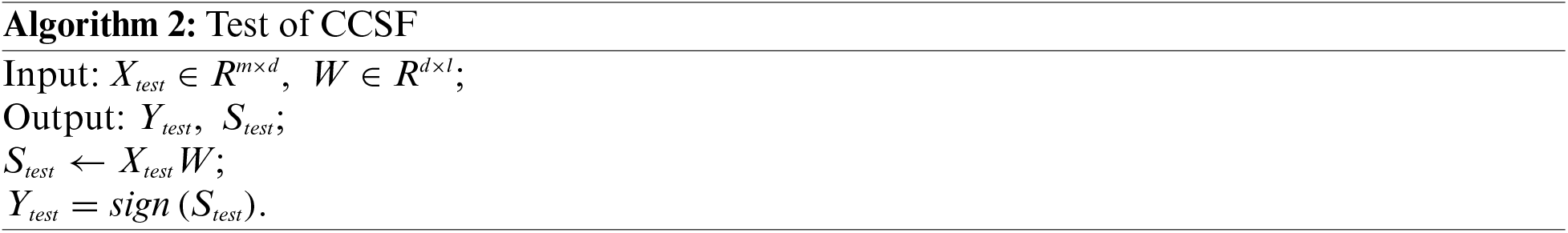
The validation method is as follows. Xtest stands for testing dataset. The matrix dimension m is the sample size of the remainder of the test set. Ytest represents predictive matrix. Stest represents score matrix.

3.3 Complexity Analysis

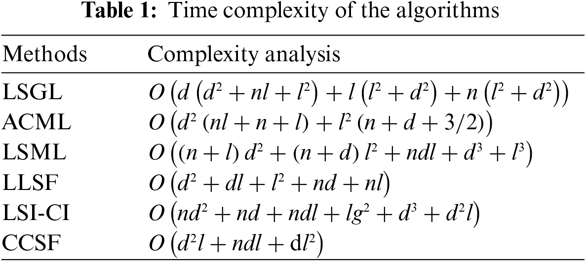
The time complexity analysis of CCSF and comparison algorithms is shown in Table 1, where n represents the number of samples, d represents the number of features, and l represents the number of labels. The time complexity of CCSF consists of computing the asymmetric correlation matrix and accelerated gradient descent method, which results in O(d2l+ndl+dl2). According to Table 1, it can be seen that the time complexity of LLSF is lower than that of CCSF, which is O(d2+dl+l2+nd+nl), but the classification effect is not as good as that of CCSF. The time complexity of FF-MLLA is not given in the article. The rest of the algorithms have higher time complexity than that of CCSF.

4  Experiment

4.1 Datasets

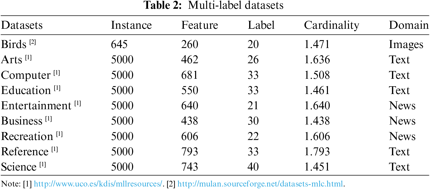
To validate the effectiveness of the algorithm proposed in this paper, five cross-validations were performed on nine multi-label benchmark datasets. The datasets are from different domains, the details of which are shown in Table 2.

4.2 Results and Comparison Algorithms

The experimental codes are implemented in MatlabR2021a, with a hardware environment of IntelCore (TM) i5-11600KF 3.90 GHz CPU, 32 G RAM, and an operating system of Windows 10.

In order to compare the effectiveness of CCSF algorithms, six commonly used evaluation metrics in MLL are selected in this paper, which are Hamming Loss (HL), Average Precision (AP), One Error (OE), Ranking Loss (RL), Coverage (CV), and AUC (AUC). Among them, the smaller the HL, OE, RL, CV metrics the better, the larger the AP and AUC metrics the better the experimental effect. Specific formulas and meanings can be found in the literature [28,29]. The parameters of the comparison algorithm are set as follows:

1) In LSGL [16] algorithm, λ1∈{10−3,10−2,…,103}, λ2,λ3,λ4,λ5∈{10−3,10−2,…,101};

2) The parameters interval of the ACML [17] algorithm are α∈[2−10,210], β∈[2−10,210];

3) Numbers of nearest neighbors in the FF-MLLA [12] algorithm are k=15, β=1, KRBF=100;

4) The parameters of LSML [15] are set as follows λ1=101, λ2=10−5, λ3=10−3, λ4=10−5;

5) The parameters of LLSF [11] are set to α=2−4, β=2−6, γ=1;

6) The parameters of LSI-CI [30] are set to α=210, β=28, γ=1, θ=2−8;

7) The parameters of CCSF are set as α, β, γ∈[2−10, 210].

The experimental results of the CCSF algorithm on 9 datasets with 6 state-of-the-art algorithms under 6 different metrics are given in Table 2, where “↑” (“↓”) indicates that higher (lower) values of the metrics are better, and the experimental results that are dominant are bolded. The details are as follows.

1) As can be seen from Table 3, out of the 54 sets of experimental results, the CCSF algorithm is superior in 49 sets, with a superiority rate of 90.74%. The CCSF algorithm significantly outperforms the other compared algorithms on all 8 datasets. The variance of the CCSF algorithm is smaller, which also proves that the CCSF algorithm is more stable. On the Birds dataset, the CCSF algorithm and the ACML algorithm are equally dominant, due to the fact that both algorithms use causal learning algorithms to compute asymmetric correlations between labels. While the Birds dataset is small, it is difficult to extract more common features of the labels, and the experimental effect dominance is not obvious compared to the larger dataset.

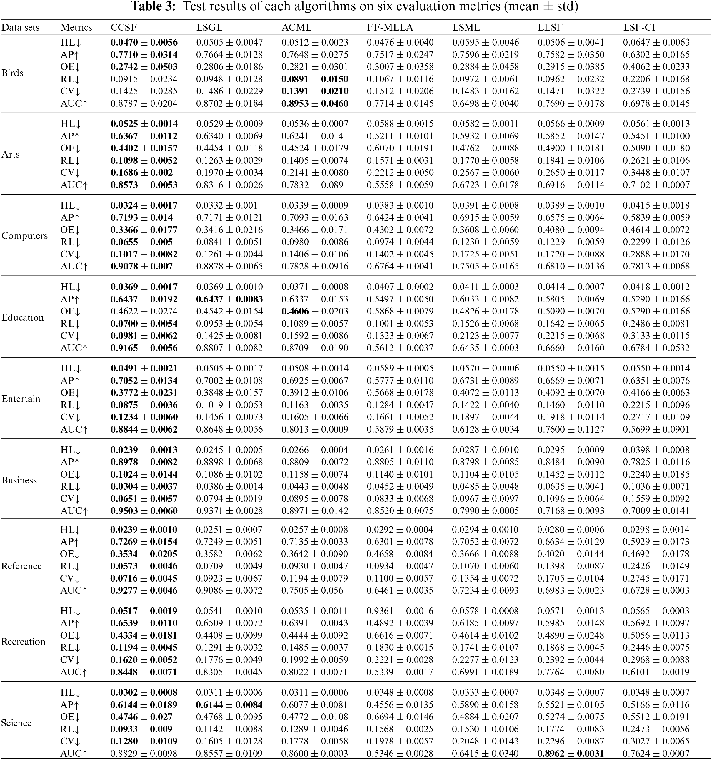
2) The CCSF algorithm significantly outperforms the ACML algorithm on these 54 sets of experimental results. This is because the ACML algorithm only takes into account the asymmetric relationship between the labels and does not take into account the fact that the common features of the labels also have a very significant role in multi-label classification.

3) The CCSF algorithm significantly outperforms the traditional LLSF algorithm and the LSGL algorithm. The reason is that the LLSF algorithm only considers the global correlation of labels. The LSGL algorithm is superior to the LLSF algorithm, which is because the LSGL algorithm not only considers the global correlation of labels, but also considers the local correlation of labels. Both of them do not consider the causal relationship between the labels and do not take into account that the common features of labels can effectively improve the performance of multi-label classification algorithms. However, we adopt a global causality and do not consider the local causality between labels, which is also a defect of the algorithm in this paper.

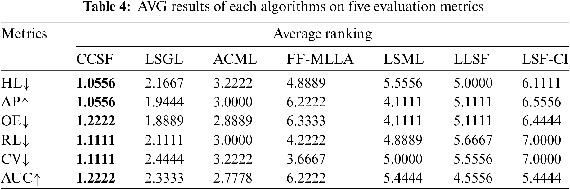
4) The experimental results of the CCSF algorithm for the average ranking of six evaluation metrics on nine datasets are demonstrated in Table 4, which also fully proves that the adoption of causal correlation and common features of labels can effectively improve the classification performance of the LSF model.

4.3 Parameter Sensitivity Analysis

The CCSF algorithm has three main hyperparameters. α and β jointly adjust the contribution of the matrix W, where α controls the contribution of the private features of the labels and β controls the contribution of the common features of the labels. γ controls the effect of asymmetric LC on the model. In order to test the sensitivity of the CCSF model, we control the other two parameters unchanged and adjust one parameter at [2−10,210] for the experiment, respectively, and the experimental results are shown in Fig. 2. χ=2x denotes the log function of log with base 2. As shown in the figure, our algorithms all have better experimental results in general, although there are some fluctuations in [2−10,210], which may also be due to the small intervals set by our algorithms. We suggest setting the parameters α=24,β=24,γ=24.

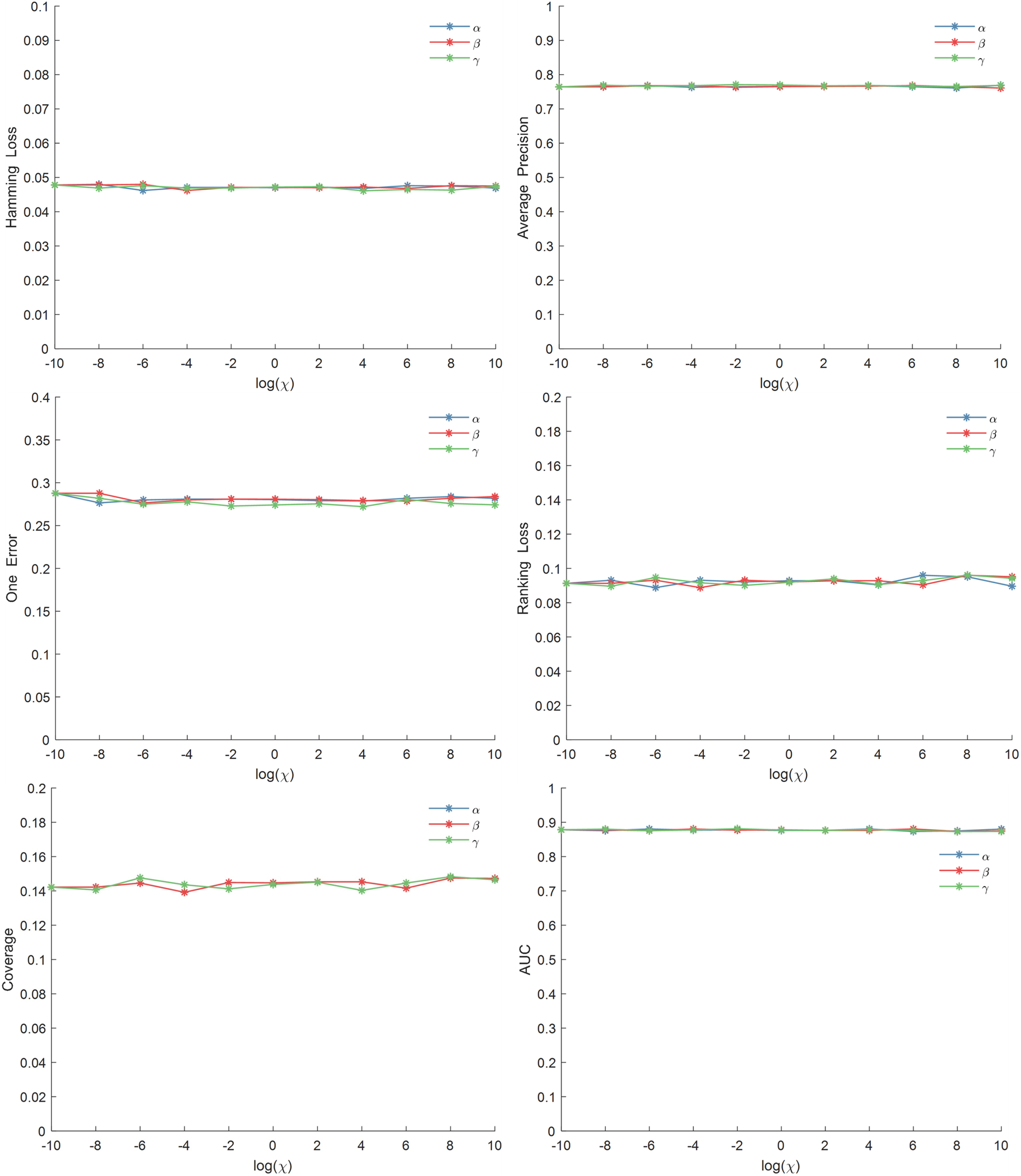
Figure 2: Parameter sensitivity analysis on the Birds dataset

4.4 Component Analysis

In order to verify that introducing common features of labels in the model can effectively improve the performance of multi-label LSF learning algorithms. We conducted component analysis experiments on nine datasets. We compare the CCSF algorithm, which combines the common and private features of label, with the CSF algorithm, which considers only the private features of label. The experimental results are shown in Fig. 3, where the CCSF algorithm outperforms the CSF algorithm on multiple datasets. This indicates that considering the common and private features of labels can effectively improve the performance of LSF algorithm. It also demonstrates that common feature learning of labels introduced into multi-label classification algorithms can improve the accuracy of the algorithms.

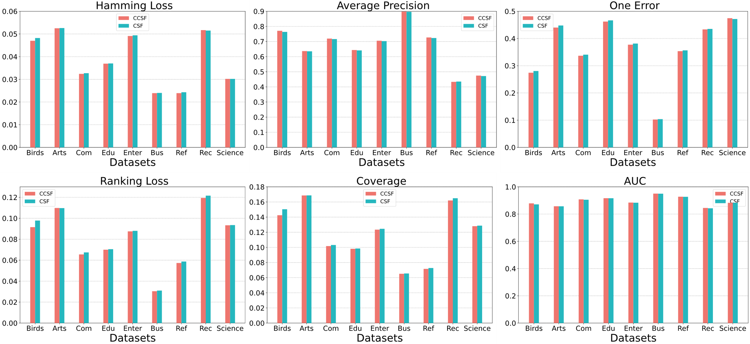
Figure 3: Component analysis on nine datasets

4.5 Statistical Hypothesis Testing

The statistical hypothesis tests in this paper are all based on a significance level of θ=0.05. The Friedman test [31] was first used to evaluate the comprehensive performance of the CCSF algorithm on all datasets. The obtained FF is compared with the critical value of the F-test. If it is greater, the original hypothesis is rejected, and vice versa. The experimental results are shown in Table 5. The FF of the CCSF algorithm is greater than the critical value for all evaluation metrics, so the original hypothesis is rejected for all of them.

Nemenyi test [32] is then used to compare the CCSF algorithm with the other six algorithms on all datasets. A significant difference exists when the difference between the average rankings of the two algorithms on all datasets is greater than the Critical Difference (CD) and vice versa. CD value is calculated as follows:

CD=qθK(K+1)6N(18)

where K=7, N=9, qθ=2.9480, CD=3.0021. Fig. 4 demonstrates the CCSF algorithm compared to other algorithms on six evaluation metrics. The algorithm performance decreases in this way from left to right. There is no significant difference between CCSF algorithm and LSGL and ACML algorithms on HL, AP, RL, CV, AUC metrics, and there is no significant difference between CCSF algorithm and LSGL, ACML, LSML algorithms on OE metrics. Other than, there is a significant difference between the CCSF algorithm and the other algorithms in six evaluation metrics. The effectiveness of the algorithm proposed in this paper can be seen from these two statistical hypothesis tests.

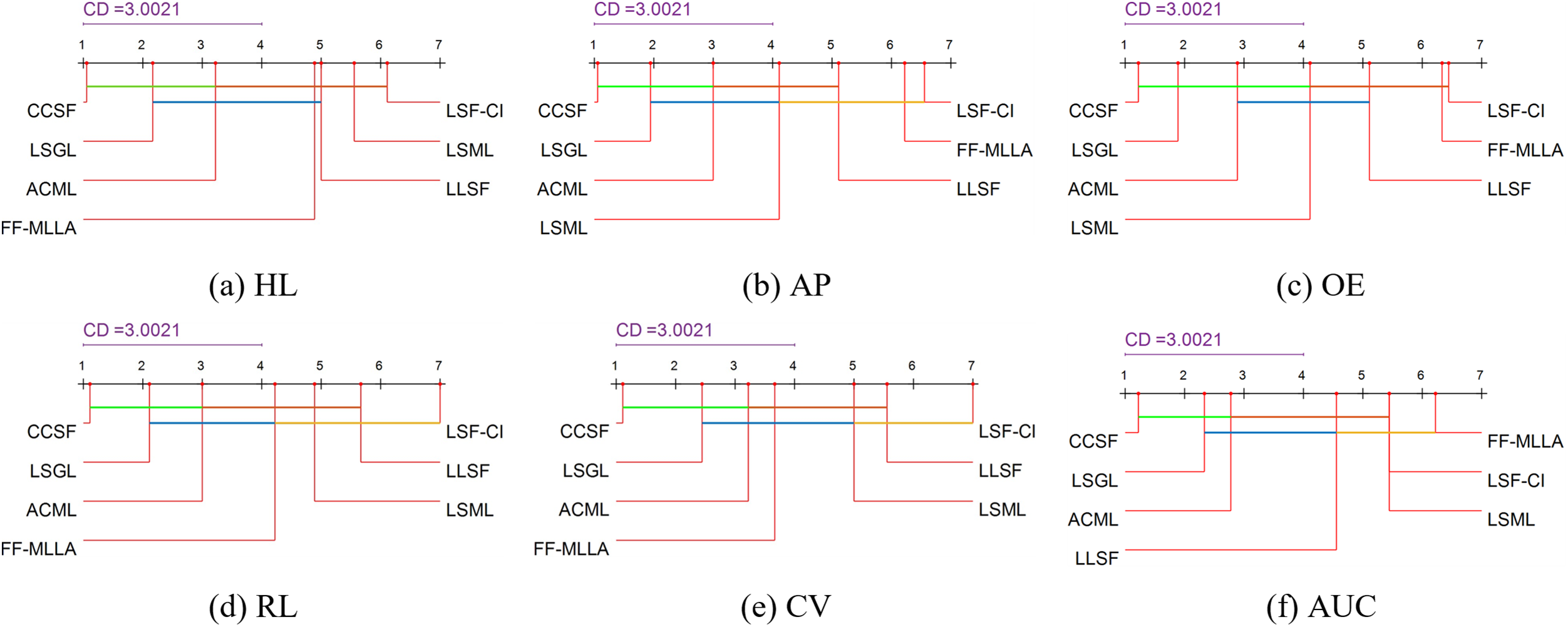
Figure 4: Performance comparison of the CCSF algorithm and the comparison algorithm

4.6 Convergence of CCSF

In this paper, the sentiment dataset and the yeast dataset are selected for convergence analysis. As can be seen in Fig. 5, after about forty iterations, the experimental results tend to converge. We conducted the same experiment on other datasets. The convergence results are also similar.

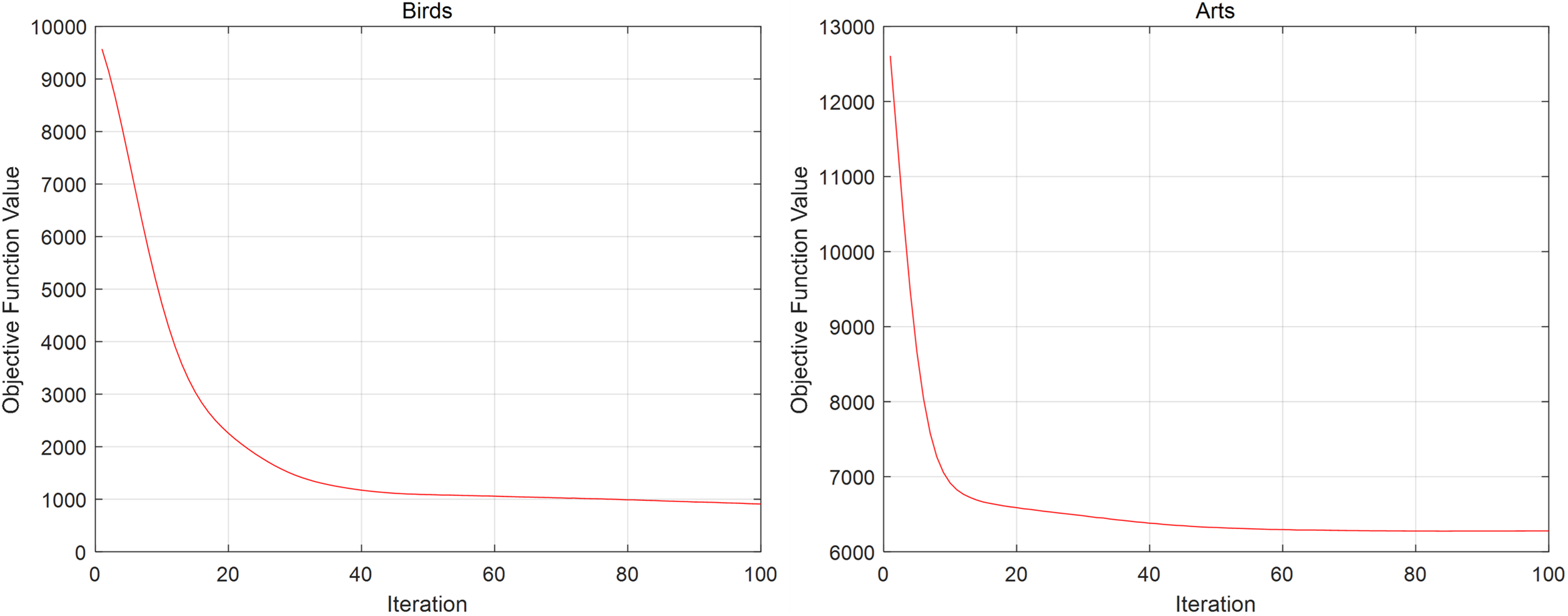
Figure 5: Convergence of CCSF

5  Conclusion

In response to the fact that most of the current LSF learning does not consider the common features of the labels. And only symmetric LC is considered in the calculation of LC. The result is the introduction of much redundant information when classification is performed, which reduces the classification performance of MLL algorithms. Based on the above problem, we use l2,1-norm and l1-norm to extract the common and private features of the labels, respectively. And the asymmetric correlation between labels is calculated utilizing the causal learning algorithm. A large number of experiments are conducted on nine datasets using six evaluation metrics, and the results prove the effectiveness of the algorithm in this paper. But at the same time, we find some problems. We use a global-based causal learning algorithm, which computes the global LC. However, some labels are only associated with local labels and only have local correlation. To minimize the complexity of the model, we also did not utilize instance correlation to improve the classification accuracy of the model. To minimize the complexity of the model, we also did not utilize instance correlation to improve the classification accuracy of the model. In the future, we will try to compute the local correlation of labels using causal learning algorithms and perform experiments in conjunction with instance correlation. We observe the results of the experiments on the complete dataset and try to solve the missing label problem.

Acknowledgement: None.

Funding Statement: 2022 University Research Priorities, No. 2022AH051989.

Author Contributions: The authors confirm contribution to the paper as follows: study conception and design: Y. T. Xu and D. Q. Zhang; analysis and interpretation of results: H. B. Guo and Y. T. Xu; draft manuscript preparation: Y. T. Xu and M. Y. Wang. All authors reviewed the results and approved the final version of the manuscript.

Availability of Data and Materials: All datasets are publicly available for download. The download URL is in Section 4.1.

Conflicts of Interest: The authors declare that they have no conflicts of interest to report regarding the present study.

References

1. M. L. Zhang and Z. H. Zhou, “A review on multi-label learning algorithms,” IEEE Trans. Knowl. Data Eng., vol. 26, no. 8, pp. 1819–1837, 2013. doi: 10.1109/TKDE.2013.39. [Google Scholar] [CrossRef]

2. W. Wei et al., “Automatic image annotation based on an improved nearest neighbor technique with tag semantic extension model,” Procedia Comput. Sci., vol. 183, no. 24, pp. 616–623, 2021. doi: 10.1016/j.procs.2021.02.105. [Google Scholar] [CrossRef]

3. T. Qian, F. Li, M. S. Zhang, G. N. Jin, P. Fan and W. Dai, “Contrastive learning from label distribution: A case study on text classification,” Neurocomput., vol. 507, no. 7, pp. 208–220, 2022. doi: 10.1016/j.neucom.2022.07.076. [Google Scholar] [CrossRef]

4. W. Q. Xia et al., “PFmulDL: A novel strategy enabling multi-class and multi-label protein function annotation by integrating diverse deep learning methods,” Comput. Biol. Med., vol. 145, pp. 105465, 2022. doi: 10.1016/j.compbiomed.2022.105465. [Google Scholar] [PubMed] [CrossRef]

5. S. H. Liu, B. Wang, B. Liu, and L. T. Yang, “Multi-community graph convolution networks with decision fusion for personalized recommendation,” in Pacific-Asia Conf. Knowl. Discov. Data Min., Chengdu, China, 2022, pp. 16–28. [Google Scholar]

6. J. L. Miu, Y. B. Wang, Y. S. Cheng, and F. Chen, “Parallel dual—channel multi-label feature selection,” Soft Comput., vol. 27, no. 11, pp. 7115–7130, 2023. doi: 10.1007/s00500-023-07916-4. [Google Scholar] [CrossRef]

7. Y. B. Wang, W. X. Ge, Y. S. Cheng, and H. F. Wu, “Weak-label-specific features learning based on multidimensional correlation,” J. Nanjing Univ. (Natural Sci.), vol. 59, no. 4, pp. 690–704, 2023 (In Chinese). [Google Scholar]

8. K. Yu et al., “Causality-based feature selection: Methods and evaluations,” ACM Comput. Surv., vol. 53, no. 5, pp. 1–36, 2020. [Google Scholar]

9. J. H. Li, P. P. Li, X. G. Hu, and K. Yu, “Learning common and label-specific features for multi-Label classification with correlation information,” Pattern Recogn., vol. 121, no. 8, pp. 108257, 2022. doi: 10.1016/j.patcog.2021.108259. [Google Scholar] [CrossRef]

10. M. L. Zhang and L. Wu, “LIFT: Multi-label learning with label-specific features,” IEEE Trans. Pattern Anal. Mach. Intell., vol. 37, no. 1, pp. 107–120, 2015. doi: 10.1109/TPAMI.2014.2339815. [Google Scholar] [PubMed] [CrossRef]

11. J. Huang, G. Li, Q. Huang, and X. D. Wu, “Learning label specific features for multi-label classification,” in 2015 IEEE Int. Conf. Data Min., Atlantic City, NJ, USA, 2015, pp. 181–190. [Google Scholar]

12. Y. S. Cheng, K. Qian, Y. B. Wang, and D. W. Zhao, “Multi-label lazy learning approach based on firefly method,” J. Comput. Appl., vol. 39, no. 5, pp. 1305–1311, 2019 (In Chinese). [Google Scholar]

13. W. Weng, Y. J. Lin, S. X. Wu, Y. W. Li, and Y. Kang, “Multi-label learning based on label-specific features and local pairwise label correlation,” Neurocomput., vol. 273, no. 9, pp. 385–394, 2018. doi: 10.1016/j.neucom.2017.07.044. [Google Scholar] [CrossRef]

14. J. Zhang et al., “Multi label learning with label-specific features by resolving label correlation,” Knowl.-Based Syst., vol. 159, no. 8, pp. 148–157, 2018. doi: 10.1016/j.knosys.2018.07.003. [Google Scholar] [CrossRef]

15. J. Huang et al., “Improving multi-label classification with missing labels by learning label-specific features,” Inf. Sci., vol. 492, no. 1, pp. 124–146, 2019. doi: 10.1016/j.ins.2019.04.021. [Google Scholar] [CrossRef]

16. D. W. Zhao, Q. W. Gao, Y. X. Lu, and D. Sun, “Learning multi-label label-specific features via global and local label correlations,” Soft Comput., vol. 26, no. 5, pp. 2225–2239, 2022. doi: 10.1007/s00500-021-06645-w. [Google Scholar] [CrossRef]

17. J. C. Bao, Y. B. Wang, and Y. S. Cheng, “Asymmetry label correlation for multi-label learning,” Appl. Intell., vol. 55, no. 6, pp. 6093–6105, 2022. doi: 10.1007/s10489-021-02725-4. [Google Scholar] [CrossRef]

18. C. Zhang, Y. S. Cheng, Y. B. Wang, and Y. T. Xu, “Interactive causal correlation space reshape for multi-label classification,” Int. J. Interact. Multimed. Artif. Intell., vol. 7, no. 5, pp. 107–120, 2022. doi: 10.9781/ijimai.2022.08.007. [Google Scholar] [CrossRef]

19. J. Luo, Q. W. Gao, Y. Tan, D. W. Zhao, Y. X. Lu and D. Sun, “Multi label learning based on double Laplace regularization and causal inference,” Comput. Eng., vol. 49, pp. 49–60, 2023 (In Chinese). [Google Scholar]

20. Y. Tan, D. Sun, Y. Shi, L. Gao, Q. Gao and Y. Lu, “Bi-directional mapping for multi-label learning of label-specific features,” Appl. Intell., vol. 52, no. 7, pp. 8147–8166, 2022. doi: 10.1007/s10489-021-02868-4. [Google Scholar] [CrossRef]

21. J. Zhang et al., “Group-preserving label-specific feature selection for multi-label learning,” Expert. Syst. Appl., vol. 213, pp. 118861, 2023. doi: 10.1016/j.eswa.2022.118861. [Google Scholar] [CrossRef]

22. L. L. Zhang, Y. S. Cheng, Y. B. Wang, and G. S. Pei, “Feature-label dual-mapping for missing label-specific features learning,” Soft Comput., vol. 25, no. 14, pp. 9307–9323, 2021. doi: 10.1007/s00500-021-05884-1. [Google Scholar] [CrossRef]

23. P. Zhao, S. Y. Zhao, X. Y. Zhao, H. T. Liu, and X. Jia, “Partial multi-label learning based on sparse asymmetric label correlations,” Knowl.-Based Syst., vol. 245, pp. 108601, 2022. doi: 10.1016/j.knosys.2022.108601. [Google Scholar] [CrossRef]

24. D. Margaritis and S. Thrun, “Bayesian network induction via local neighborhoods,” in Proc. Conf. Neural Inf. Process. Syst., Harrahs and Harveys, Lake Tahoe, USA, 2000, pp. 505–511. [Google Scholar]

25. A. Argyriou, T. Evgeniou, and M. Pontil, “Multi-task feature learning,” in Annual Conf. Neural Inf. Process. Syst., Vancouver, British Columbia, Canada, 2006, pp. 41–48. [Google Scholar]

26. A. Beck and M. Teboulle, “A fast iterative shrinkage-thresholding algorithm for linear inverse problems,” SIAM J. Imaging Sci., vol. 2, no. 1, pp. 183–202, 2009. doi: 10.1137/080716542. [Google Scholar] [CrossRef]

27. Z. C. Lin, A. Ganesh, J. Wright, L. Q. Wu, M. M. Chen and Y. Ma, “Fast convex optimization algorithms for exact recovery of a corrupted low-rank matrix,” Coordinated Sci. Lab. Report, vol. 246, pp. 2214, 2009. [Google Scholar]

28. D. W. Zhao, Q. W. Gao, Y. X. Lu, and D. Sun, “Learning view-specific labels and label-feature dependence maximization for multi-view multi-label classification,” Appl. Soft Comput., vol. 124, no. 8, pp. 109071, 2022. doi: 10.1016/j.asoc.2022.109071. [Google Scholar] [CrossRef]

29. K. Qian, X. Y. Min, Y. S. Cheng, and F. Min, “Weight matrix sharing for multi-label learning,” Pattern Recogn., vol. 136, pp. 109156, 2023. doi: 10.1016/j.patcog.2022.109156. [Google Scholar] [CrossRef]

30. H. R. Han, M. X. Huang, Y. Zhang, X. G. Yang, and W. G. Feng, “Multi-label learning with label specific features using correlation information,” IEEE Access, vol. 7, pp. 11474–11484, 2019. doi: 10.1109/ACCESS.2019.2891611. [Google Scholar] [CrossRef]

31. J. Demsar, “Statistical comparisons of classifiers over multiple data sets,” J. Mach Learn. Res., vol. 7, no. 1, pp. 1–30, 2006. [Google Scholar]

32. D. Zhao, H. Li, Y. Lu, D. Sun, D. Zhu and Q. Gao, “Multi label weak-label learning via semantic reconstruction and label correlations,” Inf. Sci., vol. 623, no. 8, pp. 379–401, 2023. doi: 10.1016/j.ins.2022.12.047. [Google Scholar] [CrossRef]