Attention-Enhanced CNN-GRU Method for Short-Term Power Load Forecasting

1  Introduction

Under the current national strategy of the “dual-carbon” goals and energy structure transformation, the power system faces multiple challenges [1,2]. On one hand, electricity demand continues to grow, especially in the context of accelerating urbanization, industrialization, and smart manufacturing, leading to a significant increase in societal power load; on the other hand, the large-scale integration of clean energy sources such as wind and solar power introduces volatility and intermittency in power supply. In this context, accurately forecasting load demand becomes a prerequisite for the safe, stable operation and scientific dispatch of the power grid [3,4].

Electric load forecasting relies on input variables such as historical electricity consumption data, meteorological conditions, and holiday effects to construct mathematical or data-driven models that forecast electricity demand for future periods [5,6]. Advances in this field can not only enhance the reliability and economic efficiency of power system operations but also effectively reduce reserve capacity, lower energy consumption, and improve generation efficiency. Therefore, developing forecasting methods that are highly accurate, intelligent, and adaptive is of critical importance for ensuring the high-quality operation of power systems [7].

Research on electric load forecasting abroad began in the early 20th century, initially focusing primarily on linear models such as regression analysis and time series models (ARIMA) [8]. Entering the 21st century, with the development of machine learning and deep learning, intelligent algorithms such as Support Vector Machines (SVM) [9], Random Forests (RF) [10], Artificial Neural Networks (ANN), and Long Short-Term Memory networks (LSTM) have gradually replaced traditional methods and become the mainstream technical approaches. The vector autoregressive hybrid model proposed in [11] can perform clustering and forecasting simultaneously, significantly improving prediction accuracy; the attention-based LSTM model in [12] further enhances the capability to model long-term dependencies; and the combination of Particle Swarm Optimization with Elman Neural Networks in [13] improves forecasting accuracy through a global optimization strategy.

Research on electric load forecasting domestically began relatively later, but has developed rapidly in recent years. Building on traditional methods, data mining and artificial intelligence techniques have been gradually introduced. In particular, with the widespread deployment of smart meters and Advanced Metering Infrastructure (AMI) systems, massive real-time data have become an important support for constructing forecasting models. In recent years, various hybrid approaches have been proposed, such as the CEEMDAN-based LSTM model in [14] and the feature-selection-based CNN-BiGRU model in [15], which have greatly improved forecasting accuracy and robustness. Nevertheless, there is still considerable room for further improvement.

This study develops a dual-input deep learning forecasting model based on multi-source time series data, integrating Convolutional Neural Networks (CNN), Gated Recurrent Units (GRU), and an attention mechanism (Attention). The model aims to fully exploit the correlations between historical load sequences and meteorological features, achieving high-accuracy forecasting of future time series data.

(1)   Data Cleaning and Feature Selection. This process consists of three main stages. First, the raw data are cleaned and processed to correct anomalies and excessive fluctuations, and temporal features such as day of the week, month, and whether it is a working day are extracted. Second, lagged statistical features are constructed for the time series data, including the mean and variance of loads over the past 1, 2, and 3 days, reflecting historical trends and volatility patterns. Finally, Pearson correlation coefficients are calculated and visualized to assess the relationships among features and between features and the target variable, providing an effective basis for subsequent feature selection.

(2)   Model Construction. One-dimensional convolutional layers (Conv1D) are first applied to extract local temporal patterns and capture short-term trend features. The GRU network is then employed to learn long-term dependencies in the time series, representing the dynamic characteristics of the sequences. Finally, a self-attention mechanism is introduced to weight the importance of different time steps, thereby focusing on key temporal features.

(3)   Experimental Comparison. The proposed model is evaluated against the aforementioned baseline models using metrics including Mean Squared Error (MSE), Root Mean Squared Error (RMSE), Mean Absolute Error (MAE), Coefficient of Determination (R2), and Mean Absolute Percentage Error (MAPE). These indicators comprehensively assess the forecasting accuracy and generalization capability of the models. Experimental results demonstrate that the method proposed in this study performs favorably compared with existing approaches.

2  Algorithm Principle

2.1 CNN Model

Convolutional Neural Networks (CNN) are a representative class of deep learning models that have been widely applied to time series analysis and forecasting in recent years. The core idea is to use local connections and weight-sharing mechanisms to extract features from input data layer by layer, thereby automatically learning spatial or temporal correlations within the data. The structure is shown in Fig. 1.

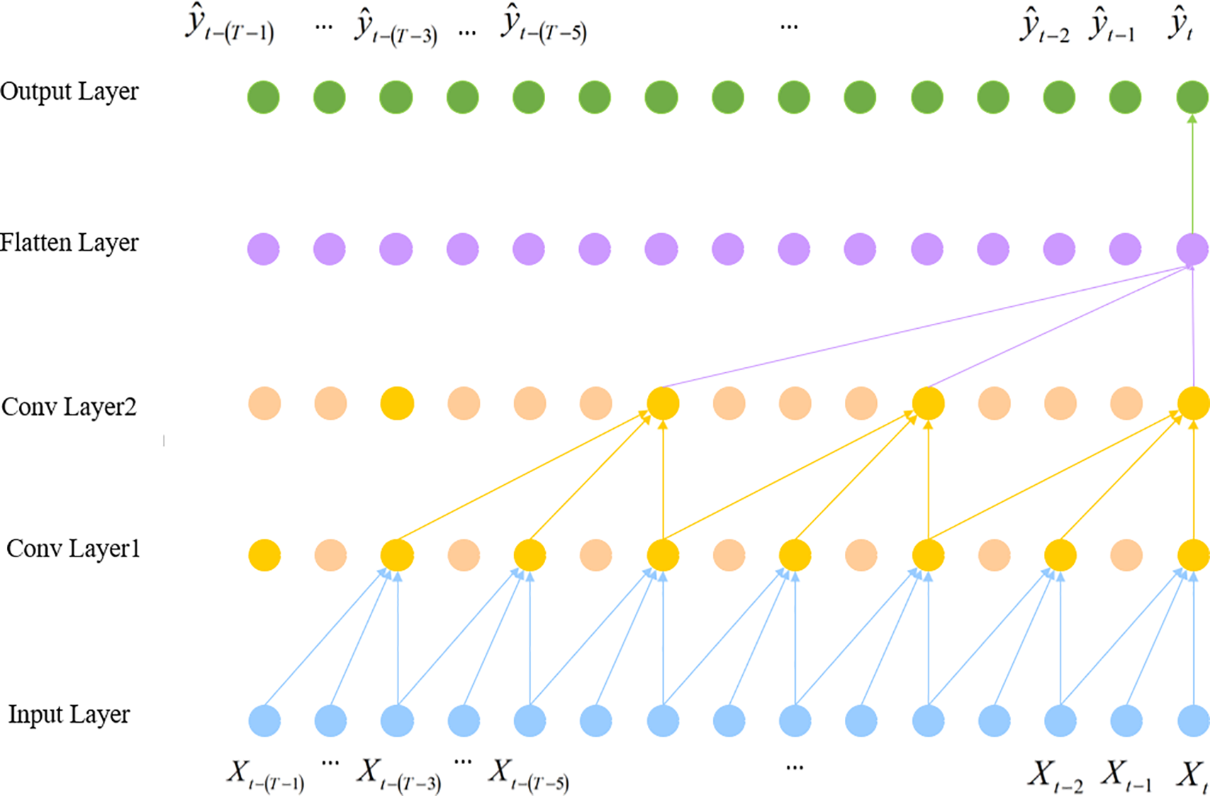
Figure 1: CNN model architecture

In the model proposed in this study, CNN is used to extract local features from the input sequences, capturing the correlations between adjacent time steps in the time series. CNN performs one-dimensional convolution on the input signals using sliding convolutional kernels, enabling automatic feature extraction and dimensionality reduction, which can effectively reduce the information loss caused by manual feature engineering. The computation formula is as follows:

First, let the input time series features be represented by a matrix X∈Rt×d, where t denotes the length of the time steps and d represents the feature dimension at each time step. Let the weight matrix of the kth convolutional kernel be W(k)∈Rs×d, then the convolution operation can be expressed as:

Zt(k)=∑i=0s−1Xt+iWi(k)+b(k)(1)

Xt+i∈R1×d denotes the input feature at the t + i-th time step, Wi(k) represents the weight of the k-th convolutional kernel at the i-th offset position, and b(k) is the corresponding bias term.

The convolution calculation slides along the time dimension to obtain the output feature sequence of the convolutional kernel:

Z(k)=[Z1(k),Z2(k),…,ZT′(k)](2)

where T ′ is the output sequence length. If using ‘same’ padding, then T ′ = T.

The convolutional output is processed through the nonlinear activation function ReLU o enhance feature representation capability. The mathematical expression for the new output features Ht(k) after ReLU processing is:

Ht(k)=ReLU(Zt(k))(3)

and ReLU(Zt(k))=max(0,Zt(k)).

If the convolutional layer has a total of K convolutional kernels, the overall output feature map H is:

H=[H(1),H(2),…,H(K)](4)

That is, each column of the output matrix corresponds to the response sequence of a convolutional kernel across the entire time dimension, while each row corresponds to the responses of different convolutional kernels at a specific time step. Here H∈Rt′×K

The output matrix H from the convolutional layer is flattened into a one-dimensional vector f through a flattening operation, facilitating subsequent concatenation and fusion with other feature branches.

f=Flatten(H)(5)

Finally, a fully connected layer is used to perform a linear mapping of the features and generate the predicted output matrix y:

y=σ(Wjf+bj)(6)

In the fully connected layer, f denotes a one-dimensional vector obtained through the flattening operation, and Wj represents a weight matrix composed of j weight vectors, which projects the feature vectors into the output space. bj denotes the bias term associated with the fully connected layer, and the σ serves as the sigmoid function.

2.2 GRU Model

GRU (Gated Recurrent Unit) is an improved variant of the Recurrent Neural Network (RNN). Its main objective is to address the vanishing and exploding gradient problems in traditional RNNs, while reducing model complexity without compromising the ability to capture long-term dependencies. The core idea of GRU is to control the flow of information through a gating mechanism. As shown in Fig. 2, the update gate determines how much of the previous hidden state should be retained and how much should be updated at the current time step. The reset gate decides how much historical information to forget, enabling the model to more flexibly capture local features.

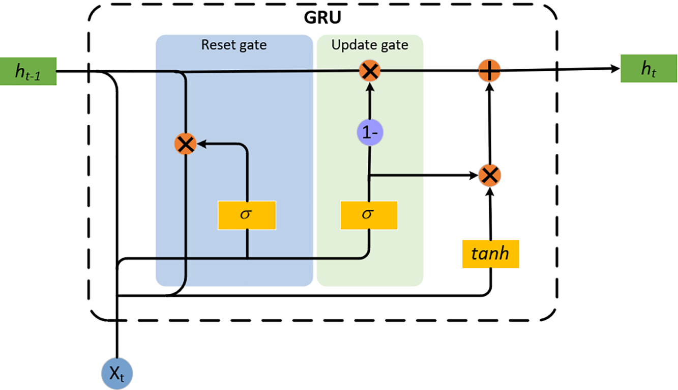
Figure 2: GRU model architecture

Given the input xt at time step t, the previous hidden state ht−1 and the current hidden state ht, the GRU model is calculated as (7)~(10):

rt=σ(Wrxt+Urht−1+br)(7)

zt=σ(WZxt+UZht−1+bZ)(8)

h∼t=tanh⁡(Whxt+Uh(rt⊙ht−1)+bh)(9)

ht=(1−Zt)⊙ht−1+Zt⊙h∼t(10)

where rt, zt, ht are reset gate, update gate and candidate hidden state, Wr, WZ, Wh, Ur, UZ, Uh, br, bZ, bh are the weight/bias matrices and vectors corresponding to each gate and the candidate state; tanh is hyperbolic tangent activation and ⊙ denotes element-wise multiplication.

2.3 Attention Mechanism

Suppose that the input sequence of attention mechanism is represented D∈Rn×c (length n, feature dimension c). Firstly, query matrix Q, key matrix K and value matrix V are obtained by linear projection:

Q=DWQ(11)

K=DWK(12)

V=DWV(13)

where, WQ, WK, WV are the projection parameters of Q, K, V.

Next, we compute the similarity S between the query and the key and scale it:

S=QKTdk(14)

here, KT refers to the transpose of the key matrix K, and dk is the attention subspace dimension.

For each query row, do softmax to get the attention weight A:

A=softmaxrow(S)(15)

Finally, the weights are normalized to obtain:

aij=exp⁡(sij)∑t=1nexp⁡(sit)(16)

Among them, aij represents the attention weight of the i-th query and the j-th one. aij ∈ [0,1]. t is the dummy variable of the summation, which traverses all positions in the row in the denominator. sij denotes the relevance of the j-th query to the j-th key i. ∑t=1nexp⁡(sit) is the normalization factor, which is used to convert the row into a probability distribution by scoring and summing the index of all key positions t (t = 1...n) for a fixed query position i.

The context representation Y (attention output) is obtained by weighted sum of the value vectors.

Y=AV(17)

3  Algorithm and General Description

Based on multi-source time series data, this paper constructs a two-input deep learning prediction model that integrates CNN, GRU and attention mechanism. The model aims to fully mine the correlation characteristics between historical load series and meteorological characteristics, and realize high-precision prediction of future time series data. The overall modeling process includes four stages: data preprocessing, feature extraction, feature fusion and output prediction, and its structure is shown in Fig. 3.

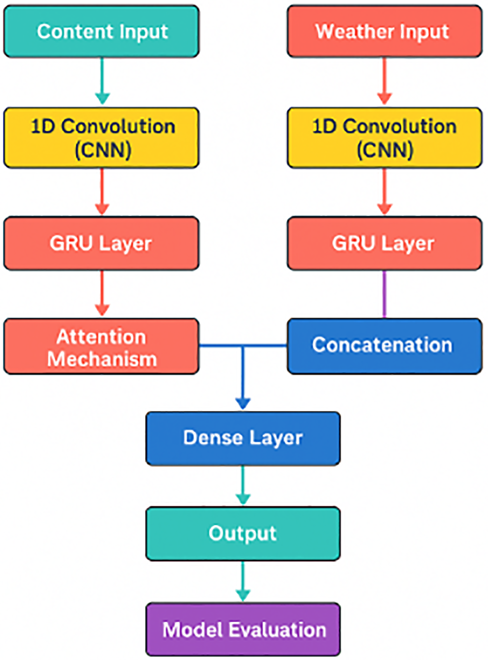
Figure 3: Structure of the method

During the data preprocessing phase, time series inputs are extracted from historical load data and meteorological features separately. A normalization technique is applied to scale each feature to the range [0,1] to eliminate the impact of dimensional discrepancies. Subsequently, the dataset is partitioned into training and test sets in an 85% to 15% ratio to ensure a reliable assessment of the model’s generalization performance.

In the feature extraction stage, the model uses a dual-input structure to process data from different sources in parallel. For the main input (content feature), the local time series pattern is extracted by Conv1D to capture the short-term trend feature. Then, GRU was used to learn the long-term dependencies in the time series to characterize the dynamic change characteristics of the series. Finally, the self-attention mechanism was introduced to weight the importance of different time steps in the sequence, so as to focus on the features at key moments. For the auxiliary input (meteorological features), the same CNN_GRU_Attention structure as the main input is used to capture the time series features and their mutual influence inside the meteorological variables.

In the feature fusion stage, the two inputs are Flatten respectively after attention weighting, and then information fusion is performed by feature Concatenate to integrate the complementary information of load features and meteorological features. The fused high-dimensional feature vector is input into two layers of fully connected network (Dense) in turn, the first layer contains 128 neurons, the second layer contains 64 neurons, and both use ReLU activation function to enhance the nonlinear mapping ability. The output layer is a Linear activation function (Linear), which is used to generate predictions 24 time steps into the future.

In the model training and optimization stage, the Mean Square Error (MSE) was used as the loss function, and the Adam optimizer was used to update the weights. The training parameters were set as follows: Batch size = 64, training Epochs = 120, and validation set proportion = 10%. The Adam optimizer comes with an adaptive learning rate mechanism that automatically adjusts the learning rate at different training stages to speed up convergence and prevent overfitting.

In the model evaluation stage, the test set is predicted and de-normalized, and a number of evaluation indicators are calculated, including mean square error (MSE), Root Mean square error (RMSE), Mean Absolute error (MAE), coefficient of determination (R2) and Mean Absolute percentage error (MAPE). These metrics are used to comprehensively evaluate the prediction accuracy and generalization ability of the model.

4  Experimental analysis

4.1 Experimental Data and Evaluation Criteria

The core data of the study were obtained from Chongqing Load Power Company in China [16], Specifically, it is the actual value of power load sampled every minute for the whole year of 2017 (January 1 to December 31), and the data scale is 525,601. This load data was randomly divided according to the ratio of 85% training set and 15% test set. The evaluation indicators selected in this paper include mean square error (MSE), Mean Absolute error (MAE), Mean Absolute percentage error (MAPE), Root Mean square error (RMSE) and coefficient of determination (R2), and the formula is as follows:

MSE=1N∑s=1N(vs−ps)2(18)

MAE=1N∑s=1N|vs−ps)|(19)

RMSE=1N∑s=1N(vs−ps)2(20)

MAPE=1N∑s=1N|vs−ps)|ps|+ε×100%(21)

R2=1−∑s=1N(vs−ps)2∑s=1N(ps−p∼)2(22)

p~=1N∑s=1Nps(23)

where N is the total number of samples. Vs is the true value of the s-th sample. ps is the predicted value of the s-th sample. p~ is the sample mean of the true values. ε is a minimal positive number.

4.2 Experimental Parameters

For a single model, the GRU model and LSTM model in literature [17], the common TCN model, the CNN model in literature [18], the XGBoost model in literature [19] and SVM model in power load data prediction are selected for experimental comparison. For the hybrid model, CNN_Attention model, CNN_BiLSTM model in literature [20], CNN_BiLSTM model and CNN_GRU model are compared. Table 1 is the experimental parameters, ensuring the same Settings for the same parameter name.

4.3 Feature Parameter Selection

In this study, the Pearson Correlation Coefficient (PCC) is employed to quantitatively analyze the relationships between electrical load and various influencing factors. After completing data cleaning and time-series alignment, a feature matrix is constructed using key variables such as historical load, temperature, and humidity. The linear correlation between each variable and the load is then calculated according to Eq. (24). To visually illustrate the correlation among variables, a correlation matrix heatmap is plotted, as shown in Fig. 4. In the heatmap, the color intensity represents the magnitude and direction of correlation, with darker colors indicating stronger correlations.

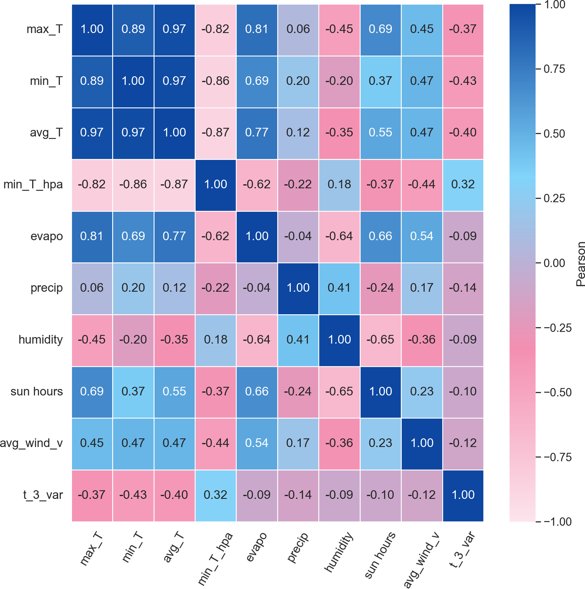
Figure 4: PCC heat map

PX,Y=∑i=1n(xi−x¯)(yi−y¯)∑i=1n(xi−x¯)2∑i=1n(yi−y¯)2(24)

Among them, the values of the i-th sample of xi and yi on the variables X and Y; x¯ and y¯ are the average values of the variables X and Y.

Based on the PCC results, variables that exhibit a strong correlation with the load are retained as model inputs, while weakly correlated or redundant features are removed. This process effectively reduces model complexity, improves training efficiency, and enhances prediction performance.

4.4 Experimental Comparison Results

Referring to Table 1, a comparative test was carried out to ensure that the Settings of the same parameter names were the same, and the experimental results were as Table 2 follows:

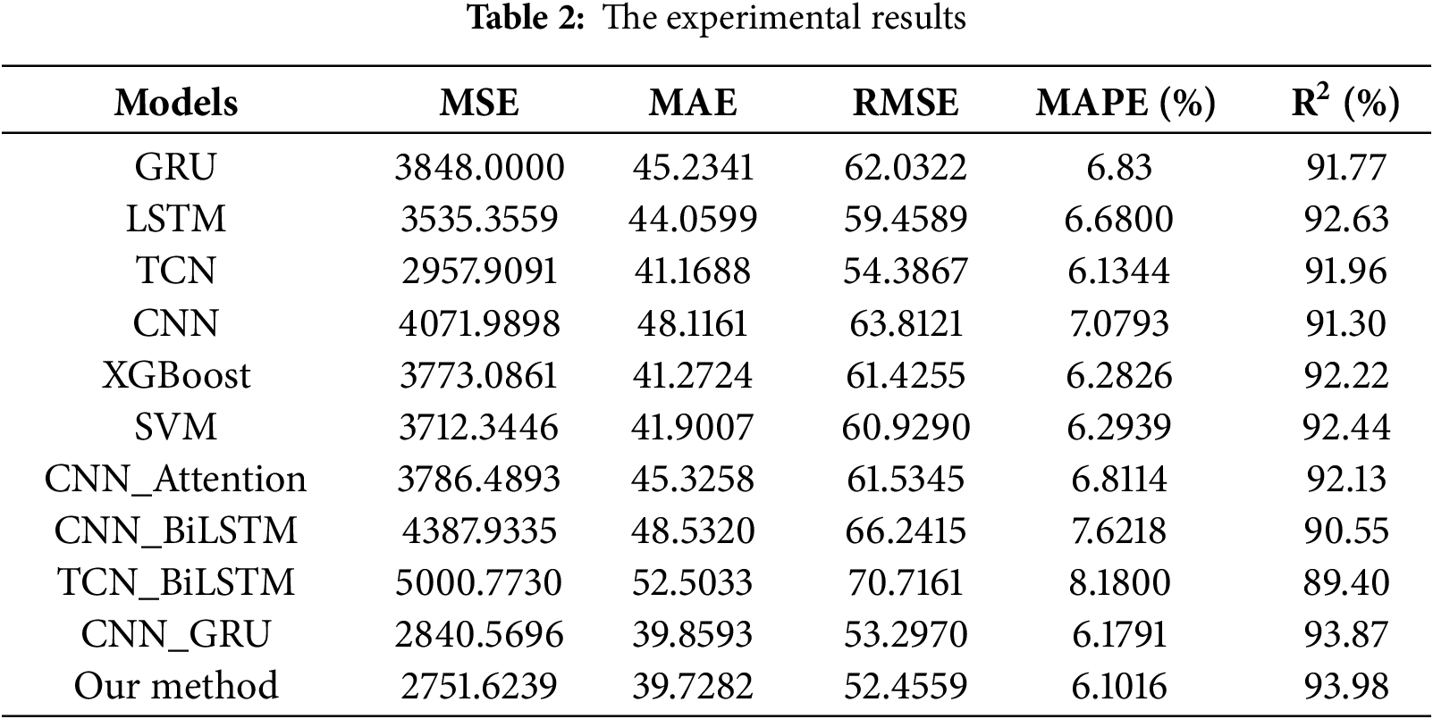
From the perspective of Mean Squared Error (MSE), the error of the proposed method in this paper is 2751.6239, which represents a decrease of 1096.38, 783.73, 206.29, 1320.37, 1021.46, 960.72, 1034.87, 1636.31, 2249.15, and 88.95 compared to GRU, LSTM, TCN, CNN, XGBoost, SVM, CNN_Attention, CNN_BiLSTM, TCN_BiLSTM, and CNN_GRU, respectively. This indicates that the proposed method achieves better stability and generalization in overall prediction error control.

In terms of Mean Absolute Error (MAE), the proposed model achieves 39.7282, representing reductions of 5.51, 4.33, 1.44, 8.39, 1.54, 2.17, 5.60, 8.80, 12.78, and 0.13 compared to the aforementioned models, further demonstrating that the model can more accurately approximate the actual load variations.

For Root Mean Squared Error (RMSE), the proposed method reaches 52.4559, which is lower than the other models by 9.57, 7.00, 1.93, 11.36, 8.97, 8.47, 9.08, 13.79, 18.26, and 0.84, showing that the model has an advantage in suppressing global prediction errors.

Regarding Mean Absolute Percentage Error (MAPE), the proposed model achieves 6.1016%, which is 0.73%, 0.58%, 0.03%, 0.98%, 0.18%, 0.19%, 0.71%, 1.52%, 2.08%, and 0.08% lower than the other models, indicating that the method also maintains high prediction accuracy on a relative error scale.

In terms of the coefficient of determination (R2), the proposed method reaches 93.98%, which is higher than the other models by 2.21, 1.35, 2.02, 2.68, 1.76, 1.54, 1.85, 3.43, 4.58, and 0.11 percentage points, demonstrating that the model can explain more of the target variance and achieves the best fitting performance.

In summary, the CNN-GRU-Attention model proposed in this paper achieves the lowest values for MSE, MAE, RMSE, and MAPE, and the highest value for R2. Its overall performance significantly outperforms traditional deep learning models and other improved models, indicating that the proposed method offers higher prediction accuracy and stronger generalization capability in the task of electric load forecasting.

5  Conclusion

The dual-input convolutional-recurrent-attention framework proposed in this paper effectively integrates complementary information from load and meteorological data: convolutional layers excel at capturing local patterns, recurrent units characterize long-term dependencies, and self-attention mechanisms highlight critical time segments while enhancing representation quality. The synergistic operation of these three components significantly reduces prediction errors and substantially improves fitting performance. The method demonstrates consistent advantages across multiple evaluation dimensions, validating the effectiveness of its architectural design and training strategy. It should be noted that explicit modeling of holiday-related abrupt changes and extreme weather events remains an area for potential improvement, while the number of attention heads and masking mechanisms also warrant further expansion. Future work could incorporate multi-head and causal masked attention mechanisms, more refined exogenous variables and prior knowledge, alongside quantile loss or Bayesian methods for uncertainty estimation, thereby further enhancing the model’s robustness and transferability in complex scenarios. The framework maintains consistent advantages across different data periods and regional power grids, demonstrating potential for engineering implementation. Furthermore, the reproducible data processing and evaluation pipeline facilitates migration to multi-industry, multi-regional scenarios, enabling continuous optimization and deployment practices while reducing maintenance costs.

Acknowledgement: The authors would like to express their gratitude for the guidance and support provided by the research group.

Funding Statement: The research work was supported in part by the Fundamental Research Funds for the Liaoning Universities (LJ212410146025), and the Innovation and Entrepreneurship Training Program for College students of University of Science and Technology Liaoning (S202510146005).

Author Contributions: Zheng Yin: Writing—original draft, Methodology, Formal analysis, Data curation. Zhao Zhang: Review and editing, Conceptualization, Supervision. All authors reviewed the results and approved the final version of the manuscript.

Availability of Data and Materials: Data and materials are available upon request.

Ethics Approval: Not applicable.

Conflicts of Interest: The authors declare no conflicts of interest to report regarding the present study.

References

1. Ten CW, Hou Y. Modern power system analysis. Boca Raton, FL, USA: CRC Press; 2024. [Google Scholar]

2. Jafarizadeh H, Yamini E, Zolfaghari SM, Esmaeilion F, El Haj Assad M, Soltani M. Navigating challenges in large-scale renewable energy storage: barriers, solutions, and innovations. Energy Rep. 2024;12(3):2179–92. doi:10.1016/j.egyr.2024.08.019. [Google Scholar] [CrossRef]

3. Ahsan F, Dana NH, Sarker SK, Li L, Muyeen SM, Ali MF, et al. Data-driven next-generation smart grid towards sustainable energy evolution: techniques and technology review. Prot Control Mod Power Syst. 2023;8(1):43. doi:10.1186/s41601-023-00319-5. [Google Scholar] [CrossRef]

4. Anushalini T, Sri Revathi B. Role of machine learning algorithms for wind power generation prediction in renewable energy management. IETE J Res. 2024;70(4):4319–32. doi:10.1080/03772063.2023.2205838. [Google Scholar] [CrossRef]

5. Kuster C, Rezgui Y, Mourshed M. Electrical load forecasting models: a critical systematic review. Sustain Cities Soc. 2017;35(11):257–70. doi:10.1016/j.scs.2017.08.009. [Google Scholar] [CrossRef]

6. Wang Z, Hong T, Li H, Ann Piette M. Predicting city-scale daily electricity consumption using data-driven models. Adv Appl Energy. 2021;2(4):100025. doi:10.1016/j.adapen.2021.100025. [Google Scholar] [CrossRef]

7. Li L, Ma W, Liu C. Optimization of power load forecasting based on big data and artificial intelligence: enhancing power system stability and operational efficiency through a systematic study. Adv Resour Res. 2025;5(2):645–65. [Google Scholar]

8. Pooniwala N, Sutar R. Forecasting short-term electric load with a hybrid of ARIMA model and LSTM network. In: Proceedings of the 2021 International Conference on Computer Communication and Informatics (ICCCI); 2021 Jan 27–29; Coimbatore, India. doi:10.1109/ICCCI50826.2021.9402461. [Google Scholar] [CrossRef]

9. Ahmad W, Ayub N, Ali T, Irfan M, Awais M, Shiraz M, et al. Towards short term electricity load forecasting using improved support vector machine and extreme learning machine. Energies. 2020;13(11):2907. doi:10.3390/en13112907. [Google Scholar] [CrossRef]

10. Azeem A, Ismail I, Jameel SM, Harindran VR. Electrical load forecasting models for different generation modalities: a review. IEEE Access. 2021;9:142239–63. doi:10.1109/access.2021.3120731. [Google Scholar] [CrossRef]

11. Li S, Kong X, Yue L, Liu C, Khan MA, Yang Z, et al. Short-term electrical load forecasting using hybrid model of manta ray foraging optimization and support vector regression. J Clean Prod. 2023;388:135856. doi:10.1016/j.jclepro.2023.135856. [Google Scholar] [CrossRef]

12. Cai C, Tao Y, Zhu T, Deng Z. Short-term load forecasting based on deep learning bidirectional LSTM neural network. Appl Sci. 2021;11(17):8129. doi:10.3390/app11178129. [Google Scholar] [CrossRef]

13. Ab Aziz MF, Mostafa SA, Foozy CFM, Abed Mohammed M, Elhoseny M, Abualkishik AZ. Integrating Elman recurrent neural network with particle swarm optimization algorithms for an improved hybrid training of multidisciplinary datasets. Expert Syst Appl. 2021;183(12–2):115441. doi:10.1016/j.eswa.2021.115441. [Google Scholar] [CrossRef]

14. Liu H, Li Z, Li C, Shao L, Li J. Research and application of short-term load forecasting based on CEEMDAN-LSTM modeling. Energy Rep. 2024;12(7):2144–55. doi:10.1016/j.egyr.2024.08.035. [Google Scholar] [CrossRef]

15. Soares LD, Franco EMC. BiGRU-CNN neural network applied to short-term electric load forecasting. Production. 2022;32:e20210087. doi:10.1590/0103-6513.20210087. [Google Scholar] [CrossRef]

16. huberyCC/Load-Datasets [Internet]. [cited 20 November 2025]. Available from: https://github.com/huberyCC/Load-datasets/tree/main/dataset2. [Google Scholar]

17. Abumohsen M, Owda AY, Owda M. Electrical load forecasting using LSTM, GRU, and RNN algorithms. Energies. 2023;16(5):2283. doi:10.3390/en16052283. [Google Scholar] [CrossRef]

18. Liu Y, Liang Z, Li X. Enhancing short-term power load forecasting for industrial and commercial buildings: a hybrid approach using TimeGAN, CNN, and LSTM. IEEE Open J Ind Electron Soc. 2023;4:451–62. doi:10.1109/ojies.2023.3319040. [Google Scholar] [CrossRef]

19. Abbasi RA, Javaid N, Ghuman MNJ, Khan ZA, Ur Rehman S, Amanullah. Short term load forecasting using XGBoost. In: Proceedings of the Workshops of the International Conference on Advanced Information Networking and Applications; 2019 Mar 27–29; Matsue, Japan. Berlin/Heidelberg, Germany: Springer; 2019. p. 1120–31. doi:10.1007/978-3-030-15035-8_108. [Google Scholar] [CrossRef]

20. Wang Y, Zhong M, Han J, Hu H, Yan Q. Load forecasting method of integrated energy system based on CNN-BiLSTM with attention mechanism. In: 2021 3rd International Conference on Smart Power & Internet Energy Systems (SPIES); 2021 Sep 25–28; Shanghai, China. doi:10.1109/spies52282.2021.9633974. [Google Scholar] [CrossRef]