On the Validity of Intermediate Tracing in Multiple Quantum Interactions

1  Introduction

Quantum interactions between multiple systems may require a large amount of computing resources, depending on the number of systems and their dimensionality. The question of at which stage to add a system to the composite system and at which state to trace it out is relevant.

Tracing out degrees of freedom is common practice in the domain of multi-system interaction. This procedure has been used in optical excitations with electron beams [1], where it is shown that the optical excitation probability from a single electron is independent of its wave function, while the probability for more (modulated) electrons depends on their relative spatial arrangement, thus reflecting the quantum nature of their interactions. Entanglement between photons induced by free electrons is analyzed in [2], showing that free electrons can control the second-order coherence of initially independent photonic states, even in spatially separated cavities that cannot directly interact. In [3], it is shown how precise control of the electron before and after its interaction with quantum light enables the extraction of the photon statistics and the implementation of full quantum state tomography using PINEM (Photon-Induced Near-field Electron Microscopy).

In previous works we dealt with such multi-system interactions as follows. In [4], we analyzed the interaction between two quantum systems: one free electron and one bound electron modeled as a two-level system (TLS). This type of interaction has been labeled FEBERI (Free-Electron Bound-Electron Resonant Interaction). The analysis delineated the particle-like and wave-like interaction regimes and discussed the possibility of using the free-electron wavepacket for interrogation and coherent control of the TLS. In [5], we analyzed the coherent excitation of a TLS by multiple free electrons modeled as quantum wave packets. To learn the accumulated effect on the TLS, we traced out the free electrons each time. We found that the transition probability of the TLS grows quadratically with the number of correlated quantum electron wavepackets (which correspond to the quadratic expansion of the sinusoidal transition rate in a Rabi oscillation process). In [6], we used the above formalism to interrogate the state of a TLS using pre-shaped free-electron quantum wavepackets. Measurement of the post-interaction energy spectrum of the free electrons probes and quantifies the full Bloch sphere parameters of the TLS. Interesting studies in electron-induced excitation of whispering gallery modes have been presented in [7–12]. In [13], we used the same formalism to examine the spontaneous emission of photons by pre-shaped quantum wave packets and analyzed the relation between the photon’s density matrix (or its Wigner distribution representation) and the quantum electron wavefunctions, which revealed the quantum-process origin of the evolution of bunched-beam superradiance. The reality of the quantum electron wave packet (QEW) and the measurability of its dimensions, as well as the transition from the quantum wave function representation to the classical point-particle theory (the wave-particle duality), were considered previously in the context of electron interactions with light [14–17].

This work is theoretical and is applicable to theoretical and computational studies. We carry out an analytic calculation which proves in general that, for the purpose of examining the results of quantum interactions between multiple systems, it is enough to add a system to the composite system before it interacts, and it is valid to trace it out after it finishes its interaction. As explained in the abstract, we consider the interaction between separate systems, meaning they are initially separable. During interaction, they usually become entangled and hence are not separable anymore, meaning that the measurement probabilities on those systems are correlated. To find out the changes on each system, we trace out the other systems and analyze each one separately, as discussed in Section 3.4. In Section 2, we carry out the analytic proof, and in Section 3, we present a numerical example with TLSs to show how this works for the simplest case of three consecutively interacting systems. The work is ended with some concluding remarks.

2  Analytic Proof

We want to examine at which stage we have to add a new system to the composite system and at which stage we may trace it out. Certainly, a system has to be present in the composite system at least during its interaction, but here we show that it has to be in the composite system only during its interaction. For this purpose, it is enough to consider two systems. The first (named below A) represents the “target” system interacting with one of the “incident” systems, and the second (named below B) is another “incident” system. We consider the density matrix of the “incident” systems to be known before the interaction; therefore, we do not evolve system B here. Therefore, the interaction happens inside system A only, and we show that its results do not depend on whether the “other” system (B) has been added to it.

We first consider system A alone, described by the density matrix ρA, dynamically changing according to the Hamiltonian HA. The evolution of A is described by the Liouville-von Neumann equation [18], in natural units (ℏ=1):

dρAdt=i(ρAHA−HAρA)(1)

If system B, described by the density matrix ρB, has been added to A, the composite system is described by the Kronecker product between the two:

ρS=ρA⊗ρB,(2)

so that the individual systems’ density matrices can be obtained by tracing over the coordinates of the “other” system:

ρA=TrBρS(3)

and

ρB=TrAρS.(4)

As shown in Eq. (1), the interactions inside system A are governed by the Hamiltonian HA. Knowing that system B does not interact with A, we could use any Hamiltonian of the type HA⊗U+U⊗HB, but as explained before, we are not interested in the evolution of B; therefore, we use the following Hamiltonian:

HS=HA⊗U,(5)

where U is the unit operator.

The equation of motion of the system S is:

dρSdt=i[ρS,HS]=i(ρSHS−HSρS)(6)

Using Eq. (2), the LHS of (6) is:

dρSdt=ddt(ρA⊗ρB)=dρAdt⊗ρB+ρA⊗dρBdt(7)

Using Eq. (5) and the mixed-product property (A⊗B)(C⊗D)=(AC)⊗(BD), the RHS of Eq. (6) consists of:

ρSHS=(ρA⊗ρB)(HA⊗U)=(ρAHA)⊗(ρBU)=(ρAHA)⊗ρB(8)

HSρS=(HA⊗U)(ρA⊗ρB)=(HAρA)⊗(UρB)=(HAρA)⊗ρB(9)

Putting those together, we obtain the equation of motion:

dρAdt⊗ρB+ρA⊗dρBdt=i(ρAHA−HAρA)⊗ρB.(10)

Tracing Eq. (10) over the coordinates of B, using the properties Trρ=1, and therefore Trdρdt=ddt Tr ρ=0, we recover Eq. (1), showing that the evolution of A is not affected by the presence of B. Tracing Eq. (10) over the coordinates of A results in:

dρBdt=0,(11)

showing that system B is not affected. In the following section, we show with a simple example how this principle works.

3  Numerical Example

We emphasize that the ideas presented in this work are general and applicable to a large series of problems, as explained in the Abstract and shown in the Introduction. We present here a simple example (out of many possible examples) to demonstrate the use of those ideas.

For this example, we use 3 qubits: A, B, and C, in a model of pure spin-spin interaction between pairs. System A is the “target” system which interacts with the others, and we could have named the “incident” systems B1 and B2, but using only 2, we name them B and C.

First, we interact qubits A and B, and after this interaction finishes, we interact qubits A and C. The Hamiltonian for the spin-spin interaction is H=σ⋅σ, where the scalar multiplication implies the sum of the Kronecker multiplications of all the Pauli matrices (in the z basis) as follows:

H=σx⊗σx+σy⊗σy+σz⊗σz=(10000−12002−100001)(12)

The Hamiltonian in Eq. (12) is diagonalizable with one eigen-energy of −3, associated with the singlet eigenvector 12(|↑↓⟩−|↓↑⟩), and three eigen-energies of 1, associated with three triplet eigenvectors: 12(|↑↓⟩+|↓↑⟩), |↑↑⟩, and |↓↓⟩ in the z basis. Therefore, the spin-spin interaction between 2 qubits is analytically solvable, and we shall use the analytic solution to check the accuracy of the numerical solutions presented here.

In this section, we present numerical solutions in 3 different policies because we need to relate to the proof in the previous section. Say we interact qubits A and B, so we may call this interacting system AB (named in Section 2 “A”). Qubit C does not interact here, so this is the “other” system (named in Section 2 “B”). Whether qubit C is part of the system as in Policies 1 and 2 or outside it as in Policy 3, the results come out identical.

The initial configuration of the qubits is shown in Fig. 1 using Bloch spheres. Qubits A, B, and C are in the positive eigenstate of σx, σy, and σz, respectively.

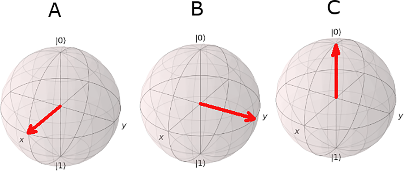
Figure 1: The initial configuration of the qubits A, B, and C: in the positive eigenstate of σx, σy, and σz, respectively. This means |ψA⟩=12(|↑⟩+|↓⟩), |ψB⟩=12(|↑⟩+i|↓⟩), and |ψc⟩=|↑⟩ in the z basis, so that the density matrices are ρA=|ψA⟩⟨ψA|, ρB=|ψB⟩⟨ψB|, and ρC=|ψC⟩⟨ψC|.

To run an interaction, we implement the equation of motion using the following recursion, which is the numerical solution to the Liouville-von Neumann equation [18]:

ρ(n+1)=ρ(n)+idt(ρ(n)H−Hρ(n))(13)

which can be improved using the trapezoidal rule [19], but this will suffice for our purpose. We shall run Eq. (13) for 500 steps; each step advances the time by dt=1×10−4 (in natural units ℏ=1). This means that we run the system for a time interval of 500×10−4=0.05, which is short, and therefore the deviation from the initial state is small. We shall run the interactions first between A and B and then between A and C, using 3 different policies of adding or tracing out qubits, as shown in the subsections below.

3.1 Policy 1

We show here the least efficient policy, shown in Fig. 2, which keeps all components in the system during all interactions.

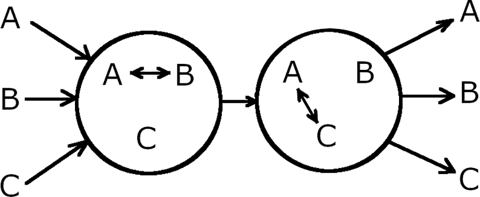
Figure 2: Policy 1: we combine all the systems, carry out both interactions, and at the end trace out everything.

We combine the whole system of 3 qubits:

ρABC=ρA⊗ρB⊗ρC(14)

Then we interact A with B, using:

H=σ⋅σ⋅1=σx⊗σx⊗U+σy⊗σy⊗U+σz⊗σz⊗U(15)

After this interaction finished, we interact A and C, using:

H=σ⋅1⋅σ=σx⊗U⊗σx+σy⊗U⊗σy+σz⊗U⊗σz(16)

At the end, we partial trace:

ρA=TrBC{ρABC};ρB=TrAC{ρABC};ρC=TrAB{ρABC}(17)

3.2 Policy 2

This policy, shown in Fig. 3, has a better efficiency than the previous one, but is not the best possible.

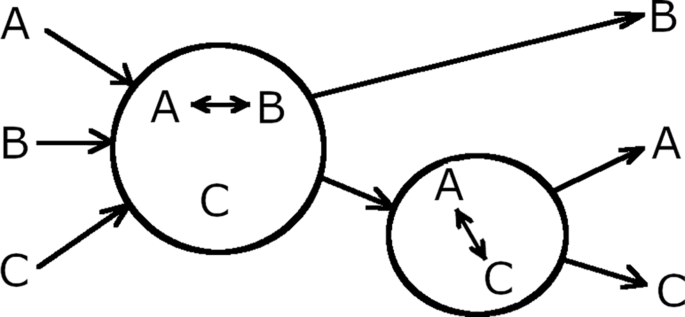
Figure 3: Policy 2: we combine all the systems and carry out the A–B interaction. We trace out B and carry out the A–C interaction on the reduced A–C system.

Like in the previous policy, we build the whole system:

ρABC=ρA⊗ρB⊗ρC(18)

and interact A with B, using:

H=σ⋅σ⋅1=σx⊗σx⊗U+σy⊗σy⊗U+σz⊗σz⊗U.(19)

Unlike the previous case, after this interaction finished, we trace out B, obtaining the density matrix of system AC:

ρAC=TrB{ρABC}(20)

and trace out AC to obtain the density matrix of B:

ρB=TrAC{ρABC}(21)

The advantage of this policy vs. the previous one is in the interaction that follows; we use only 2 qubits instead of 3. So we interact the system of 2 qubits AC, using:

H=σ⋅σ=σx⊗σx+σy⊗σy+σz⊗σz(22)

At the end, we partial trace to obtain the density matrices of A and C:

ρA=TrC{ρAC};ρC=TrA{ρAC}(23)

3.3 Policy 3

This is the most efficient policy, shown in Fig. 4; we keep each time only the interacting components.

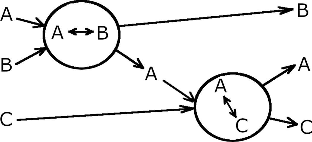
Figure 4: Policy 3: we combine A–B, carry out the A–B interaction, and trace out A and B. Then we combine A–C to carry out the A–C interaction.

First, we build the partial system AB:

ρAB=ρA⊗ρB,(24)

and interact A with B, using:

H=σ⋅σ=σx⊗σx+σy⊗σy+σz⊗σz(25)

After interaction finished, we trace out B, remaining with:

ρA=TrB{ρAB}(26)

and trace out A, obtaining:

ρB=TrA{ρAB}.(27)

Now we build the system:

ρAC=ρA⊗ρC,(28)

and interact A with C, using the above Hamiltonian. At the end, we partial trace to obtain the density matrices for A and C:

ρA=TrC{ρAC};ρC=TrA{ρAC}(29)

As the theory predicts, all three policies give identical results for the 3 qubits. We show the results in Bloch sphere parameters rather than density matrices because they are easier to visualize. The results expressed as radius (r), elevation angle in degrees (θ), and azimuth angle in degrees (φ) are:

Qubit A:

r=0.98913θ=95.072φ=6.3053(30)

Qubit B:

r=0.99507θ=84.299φ=89.424(31)

Qubit C:

r=0.99399θ=8.481φ=−83.706(32)

As previously explained, the spin-spin interaction between two qubits is solvable analytically; we therefore were able to verify the accuracy of the above numerical results. Their accuracy is better than 10−6.

The comparison between the run time of those algorithms shows that Policy 2 is by 30% more effective than Policy 1, and Policy 3 is 60% more effective than Policy 1, which makes sense because in Policy 2 we made one calculation more efficient, while in Policy 3 we made the calculations for both interactions more efficient.

We can give a general estimate for successive interactions on how much computer time we save. Say the target system (in our example, system A) is of dimension N and there are L incident systems (in our example, systems B and C), each of dimension M. Combining all the systems (as in Policy 1), we get a composite system of dimension K=MLN. Calculations (as described in Eq. (1), and solved iteratively as in Eq. (13)) require multiplications of K×K matrices; each such multiplication requires K3=(MLN)3 operations. We calculate L interactions, with s steps each, resulting in sL(MLN)3 operations.

Alternatively, using Policy 3, we also calculate L interactions, with s steps each, but on matrices of dimension MN, each multiplication requiring (MN)3 operations, resulting in sL(MN)3 operations. Hence, we save by a ratio of M3(L−1). In the small example shown here, M=2 and L=2, we save by a factor of 8 (but there is an overhead of Kronecker multiplications and partial tracing, so the saving is less). This fits the comparison between the run time of the different policies mentioned above.

Applying the above calculation for the interactions in [5], in which we interacted L=50 free electrons with Gaussian quantum wavefunction modeled with M=20, we saved by a ratio of 203×49, which is practically infinite. In other words one could not have done the calculation in [5] without “add and trace”.

The results are shown in Fig. 5; the red arrows show the state of the qubits after interaction, and the white arrows (for reference) show the state of the qubits before interaction.

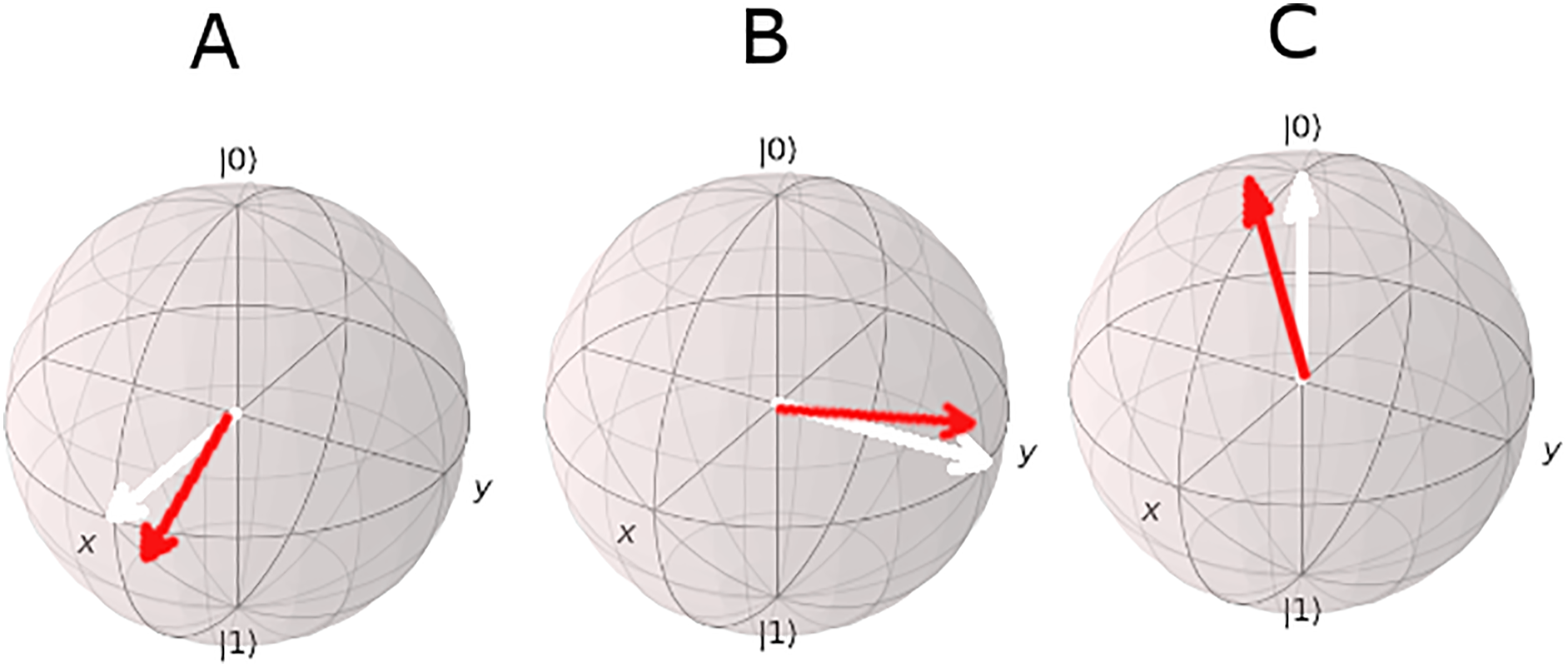
Figure 5: The 3 qubits after the completion of all interactions; their states are marked by the red arrows. For reference, the white arrows show the states of the qubits before interaction, and as mentioned, we used short-term interactions; hence, the differences are small.

3.4 Analysis of the Results

We interpret here the results of the above interactions. The probability to measure a qubit in the positive eigenstate of σi (for i=x,y or z) is given by:

Pi=Tr{ρ(U+σi)/2}(33)

where ρ is the density matrix of the qubit. The probabilities for each of the qubits are computed and shown in Table 1.

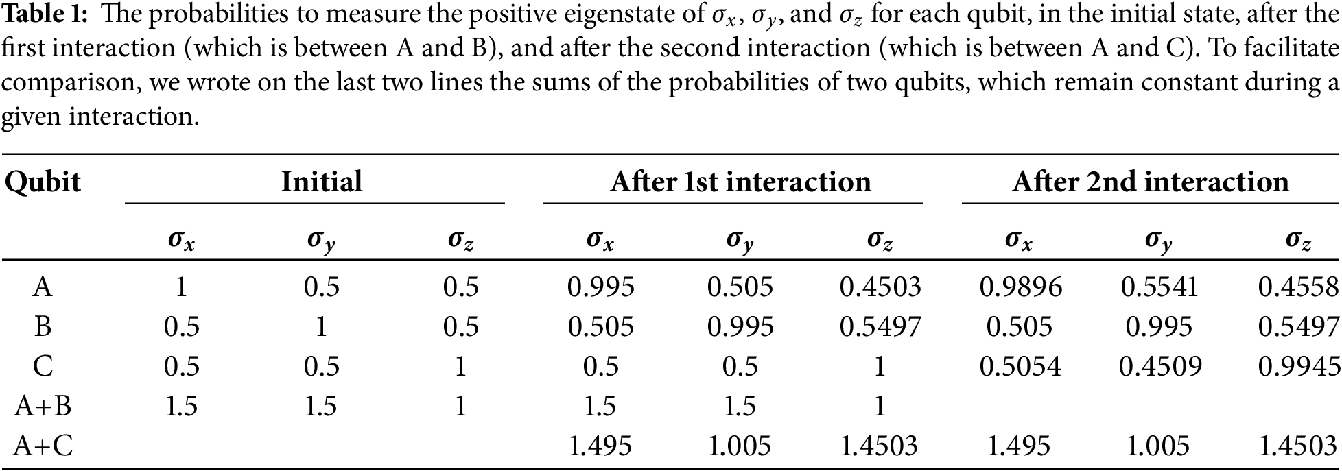
At the initial state, each qubit has a probability of 1 to be measured along the axis on which it has been prepared (qubit A along the x axis, qubit B along y, and qubit C along z), and 0.5 along any other axis (see Fig. 1). The first interaction is between A and B; hence, C is unaffected. After the first interaction, A’s probability to be in the positive eigenstate of σx decreases, and so does B’s probability to be in the positive eigenstate of σy by the same amount. Each one acquires some of the property of the other: A and B have now a small probability to be in the positive eigenstate of σy and σx, respectively. There is also a probability exchange in the positive eigenstate of σz.

The second interaction is between A and C, so that B remains unaffected. A and C exchange some probability to be in the positive eigenstate of σx, where A loses what C gains, in the positive eigenstate of σy, where C loses what A gains, and in the positive eigenstate of σz, where C loses what A gains.

4  Discussion

We analyzed in this work the policy of adding and tracing out quantum systems for handling multiple interactions of such systems. The conclusion is that a system should be part of a larger system only during the time it interacts. In other words, it may be added before its interaction and traced out after its interaction. We gave an analytic proof of this property and showed a numerical example to demonstrate this principle.

In the context of the FEBERI (free-electron bound-electron resonant interaction) process of multiple modulation-correlated quantum electron wavefunctions interacting with a TLS [4,6], the lesson of this derivation is that the procedure used, of partial tracing of the bound-electron state after each interaction, is valid for evaluating the Rabi oscillation evolution of the TLS under a stream of interacting electrons (or its quadratic expansion when starting from the ground state [5]). In this problem, the state of the expired electron is traced out after each electron-TLS dual interaction, and the revised TLS state is used for calculating the interaction with the next electron.

Likewise, in the context of the interaction of multiple modulation-correlated quantum electron wavefunctions with a radiation mode and the evolution of bunched-beam superradiance [13], the expired electron is traced out after each interaction to provide the updated quantum state of the radiation mode for use in the interaction with the next electron. This provides the evolution of the radiation mode quantum state under the stream of the electrons and the Dicke-type quadratic growth of the photon number with the number of electrons starting from a vacuum state. This technique has been implemented for excitation of photonic nanostructures with free electrons [1] and for coherent excitation of a bound electron (modeled as a two level system) by multiple free electrons quantum wave packets [5]. These procedures are only limited by the requirement that there is no more than a single electron in the interaction region during its interaction time.

Typically the “incident” systems are considered far from one another (in time and space), so that one is interested in the cumulative effect of them on the “target” system, therefore we discussed examples of two interacting systems at a time. But we shall emphasize that the analytic proof shows that anything that is not interacting can be outside the combined system of interacting elements (which may be more than 2 systems). Hence, the proof is applicable to more scenarios: for example, incident systems B1, B2,..., Bn and target A, where the interaction is sequentially between 3 systems (Bk−1, Bk, A followed by Bk, Bk+1, A, and so on). The important thing is to include only the interacting systems at a time. This method is irrelevant only in the case all the systems involved co-interact at all times.

This work also relates to quantum communication and key distribution [20,21], which involves interacting quantum systems, purifying quantum states [22], partial tracing and recombination, and to modeling and control of quantum systems in what concerns the ability of employing quantum systems to store, manipulate and retrieve information [23]—e.g., the problem solved here in Section 3.

Acknowledgement: None.

Funding Statement: This research was funded by Israeli Science Foundation grant number ISF 2992/24.

Author Contributions: The authors confirm contribution to the paper as follows: Conceptualization, Reuven Ianconescu, Bin Zhang and Avraham Gover; methodology, Reuven Ianconescu and Bin Zhang; writing—original draft preparation, Reuven Ianconescu; writing—review and editing, Reuven Ianconescu, Jacob Scheuer and Avraham Gover; supervision, Aharon Friedman and Avraham Gover. All authors reviewed and approved the final version of the manuscript.

Availability of Data and Materials: Not applicable. This article does not involve data availability, and this section is not applicable.

Ethics Approval: Not applicable for studies not involving humans or animals.

Conflicts of Interest: The authors declare no conflicts of interest.

Abbreviations

References

1. de Abajo FJG, Giulio VDi. Optical excitations with electron beams: challenges and opportunities. ACS Photonics. 2021;8:4–974. doi:10.1021/acsphotonics.0c01950. [Google Scholar] [PubMed] [CrossRef]

2. Baranes G, Ruimy R, Gorlach A, Kaminer I. Free electrons can induce entanglement between photons. npj Quantum Inf. 2022;8(1):32. doi:10.1038/s41534-022-00540-4. [Google Scholar] [CrossRef]

3. Gorlach A, Karnieli A, Dahan R, Cohen E, Pe’er A, Kaminer I. Ultrafast non-destructive measurement of the quantum state of light using free electrons. arXiv:2012.12069. 2020. [Google Scholar]

4. Zhang B, Ran D, Ianconescu R, Friedman A, Scheuer J, Yariv A, et al. Quantum wave-particle duality in free-electron-bound-electron interaction. Phys Rev Lett. 2021;126:244801. doi:10.1142/9789812817426_0006. [Google Scholar] [CrossRef]

5. Ran D, Zhang B, Ianconescu R, Friedman A, Scheuer J, Yariv A, et al. Coherent excitation of bound electron quantum state with quantum electron wavepackets. Front Phys. 2022;10:920701. doi:10.3389/fphy.2022.920701. [Google Scholar] [CrossRef]

6. Zhang B, Ran D, Ianconescu R, Friedman A, Scheuer J, Yariv A, et al. Quantum states interrogation using a pre-shaped free electron wavefunction. Phys Rev Res. 2022;4:033071. [Google Scholar]

7. Auad Y, Hamon C, Tencé M, Lourenço-Martins H, Mkhitaryan V, Stéphan O, et al. Unveiling the coupling of single metallic nanoparticles to whispering-gallery microcavities. Nano Lett. 2022;22:319–27. doi:10.1021/acs.nanolett.1c03826. [Google Scholar] [PubMed] [CrossRef]

8. Müller N, Hock V, Koch H, Bach N, Rathje C, Schäfer S. Broadband coupling of fast electrons to high-Q whispering-gallery mode resonators ACS. Photonics. 2021;8:1569–75. doi:10.1021/acsphotonics.1c00456. [Google Scholar] [CrossRef]

9. Kfir O. Entanglements of electrons and cavity photons in the strong-coupling regime. Phys Rev Lett. 2019;123:103602. doi:10.1103/PhysRevLett.123.103602. [Google Scholar] [PubMed] [CrossRef]

10. Kfir O, Lourenço-Martins H, Storeck G, Sivis M, Harvey TR, Kippenberg TJ, et al. Controlling free electrons with optical whispering-gallery modes. Nature. 2020;582:46–9. doi:10.1038/s41586-020-2320-y. [Google Scholar] [PubMed] [CrossRef]

11. Kfir O, Giulio VDi, de Abajo FJG, Ropers C. Optical coherence transfer mediated by free electrons. Sci Adv. 2021;7:eabf6380. doi:10.1126/sciadv.abf6380. [Google Scholar] [PubMed] [CrossRef]

12. Karnieli A, Rivera N, Arie A, Kaminer I. The coherence of light is fundamentally tied to the quantum coherence of the emitting particle. Sci Adv. 2021;7:eabf8096. doi:10.1126/sciadv.abf8096. [Google Scholar] [PubMed] [CrossRef]

13. Zhang B, Ianconescu R, Friedman A, Scheuer J, Tokman M, Pan Y, et al. Spontaneous photon emission by shaped quantum electron wavepackets and the QED origin of bunched electron beam superradiance. Rep Prog Phys. 2024;88(1):017601. doi:10.1088/1361-6633/ad9052. [Google Scholar] [PubMed] [CrossRef]

14. Fares H. The quantum effects in slow-wave free—electron lasers operating in the low-gain regime. Phys Lett A. 2020;384(35):126883. doi:10.1016/j.physleta.2020.126883. [Google Scholar] [CrossRef]

15. Corson JP, Peatross J, Müller C, Hatsagortsyan KZ. Scattering of intense laser radiation by a single-electron wave packet. Phys Rev A. 2011;84:053832. doi:10.1103/physreva.84.053831. [Google Scholar] [CrossRef]

16. Kaminer I, Mutzafi M, Levy A, Harari G, Sheinfux H, Skirlo S, et al. Quantum cerenkov radiation: spectral cutoffs and the role of spin and orbital angular momentum. Phys Rev X. 2016;6:011006. [Google Scholar]

17. Remez R, Karnieli A, Trajtenberg-Mills S, Shapira N, Kaminer I, Lereah Y, et al. Observing the quantum wave nature of free electrons through spontaneous emission. Phys Rev Lett. 2019;123:060401. doi:10.1103/PhysRevLett.123.060401. [Google Scholar] [PubMed] [CrossRef]

18. Messiah A. Quantum mechanics. Vol. 1. Amsterdam, The Netherland: North-Holland Publishing Company; 1962. [Google Scholar]

19. Trefethen LN, Weideman JAC. The exponentially convergent trapezoidal rule. SIAM Rev. 2014;56(3):385–458. doi:10.1137/130932132. [Google Scholar] [CrossRef]

20. Sasikumar S, Sundar K, Jayakumar C, Obaidat MS, Stephan T, Hsiao KF. Modeling and simulation of a novel secure quantum key distribution (SQKD) for ensuring data security in cloud environment. Simul Model Pract Theory. 2022;121:102651. doi:10.1016/j.simpat.2022.102651. [Google Scholar] [CrossRef]

21. Sharma A, Kaur S. Performance investigation of quantum key distribution system through free-space optics. Optik. 2025;339:172535. doi:10.1016/j.ijleo.2025.172535. [Google Scholar] [CrossRef]

22. Carle T, Kraus B, Dür W, de Vicente JI. Purification to locally maximally entangleable states. Phys Rev A—Atomic Molec Optic Phy. 2013;87(1):012328. doi:10.1103/physreva.87.012328. [Google Scholar] [CrossRef]

23. Altafini C, Ticozzi F. Modeling and control of quantum systems: an introduction. IEEE Trans Automat Contr. 2012;57(8):1898–917. doi:10.1109/tac.2012.2195830. [Google Scholar] [CrossRef]