An ADRC Parameters Self-Tuning Control Strategy of Tension System Based on RBF Neural Network

1  Introduction

The roll-to-roll precision coating machine is ideal equipment for mass manufacturing of printed electronic products, but the manufacture of printed electronic devices puts forward higher requirements for the coating machine. Tension control precision is one of the most important indexes to produce printed electronic devices and the key factor that restricts the application of precision coating machines in the printed electronics field. However, the tension system has the characteristics of nonlinear, strong coupling, numerous interference factors, and time-varying parameters, which make high-precision tension control very difficult. Existing tension control strategies based on PID cannot meet the tension control requirements of the precision coating machine. Therefore, it is necessary to design a tension control strategy that can realize the decoupling control of the precision coating machine tension system.

The tension control of the roll-to-roll system has always been a research hotspot of scholars. To solve the problem of insufficient tension control accuracy, researchers in various countries have carried out in-depth research in this field. Currently, PID is still the most widely used tension control method in the industry, and there are many improved control methods for PID to achieve tension control [1–4]. With the development of computer technology and modern control theory, modern control methods such as robust control and neural network control are gradually applied in the field of tension control for the roll-to-roll system. Jiang designed a sliding mode controller for controlling the diaphragm tension in the unwinding process [5]. Chen et al. [6] designed a robust decentralized H∞ controller to attenuate tension fluctuations introduced by the external disturbances and interaction between two consecutive subsystems. Kuznetsov et al. [7] developed a method of feedforward robust stochastic anisotropic control synthesis by cable winding machine. Liu et al. [8] designed full-order state observers and adaptive robust controllers for the rolling mill system’s speed and tension outside the loop. Talian et al. [9] designed a stable and robust tension controller for the middle sections of continuous lines on basis of the second Lyapunov method. Although many studies have applied modern control strategies to tension control, it requires a large amount of model information, and it is difficult to establish accurate models for systems in industrial practice. Therefore, it is necessary to use a model-independent high-precision decoupling control algorithm to cope with the complexity of tension system. The Active Disturbance Rejection Control (ADRC) can realize real-time estimation and compensation of internal and external disturbances in the system, because of its good dynamic characteristics, it has been used in many fields [10–13]. There are also several studies on the application of ADRC for tension system control. Meng proposed the method combined with seeker optimization algorithm and ADRC for tension control [14]. Liu et al. [15,16] respectively proposed a decoupling controller based on ADRC to solve the problem of tension control for unwinding and rewinding tension system of gravure printing machines. Zhang et al. [17] considered the parameter uncertainty and the multi-disturbance of the stainless-steel strip processing line and designed an ADRC controller. In recent years, RBF neural network has been widely used in the field of controller parameter adjustment due to its advantages including strong generalization capability, fast convergence, and high approximation accuracy for parametric time-varying systems. Yin et al. [18] designed a fractional-order PID controller based on neural network self-anti-disturbance control for rocket artillery AC servo nonlinear systems. Kumar et al. [19] compared RBF with other methods (BP neural network, etc.) to verify that RBF is more accurate in controlling nonlinear systems. Li et al. [20] applied RBF neural network to the motor motion controller to enhance the adaptiveness and robustness of the servo system.

The purpose of this study is to design an integrated decoupling control strategy based on feedforward control, ADRC and RBF neural network to improve the control accuracy of the tension system in roll-to-roll precision coating machine. The structure is as follows: Section 2 describes the tension system structure of the precision coating machine and establishes a global coupling model of the tension system which is linearized based on the first-order Taylor formula. Section 3 proposes a parameters self-tuning decoupling algorithm of the tension system by integrating feedforward control, ADRC and RBF neural network, and designs a tension observer for dancer roll. To test the effectiveness of the proposed decoupling strategy, simulations and analysis compared with PID and ADRC controllers are carried out in Section 4. Section 5 summarizes the controller performance and gives directions for future work.

2  Global Model of Tension System

2.1 Tension System Structure of Roll-to-Roll Precision Coating Machine

Fig. 1 shows the structure of the tension system, L1~L6 are respectively the length of the substrate of each span, T1~T6 are respectively the tension of the substrate of each span, and ω1~ω7 are respectively the motor speed of each unit. According to the functions realized by different parts, the tension system is divided into three subsystems: unwinding subsystem, coating subsystem, and rewinding subsystem. The specific components of each tension subsystem are marked, and every unit is driven by servo motors. As the structure is shown in Fig. 1, the tension spans from left to right are unwinding span, infeeding span, coating span, cooling span, outfeeding span, and rewinding span. A multistage oven system is arranged in the cooling span to dry the coated substrate. It can be seen that the substrate starts from the unwinding unit and is gradually transferred to each subsequent functional unit at a certain speed, during which the tension will also be propagated to the subsequent units with the movement of the substrate. The substrate tension of each span is continuous, and there is a coupling effect between each tension span, the change of the tension in the previous span will inevitably affect the subsequent spans. In addition, from the infeeding unit to the outfeeding unit, the motor speed of each unit exists in both the front and rear tension spans, and the coupling of the motor speed of the unit exists between the two adjacent spans. Therefore, to control the tension precisely, it is necessary to propose a control strategy that can realize the decoupling of tension.

Figure 1: The structure of the tension system

At present, the tension detection devices widely used in the precision coating machine include dancer roll and load cell. As the coating machine structure is shown in Fig. 1, the load elements are arranged in the infeeding span, the coating span, and the cooling span respectively. The dancer rolls are installed in the unwinding span, the outfeeding span, and the rewinding span respectively. The dancer roll has the functions of tension detection and tension mutation suppression at the same time and has been widely used in various printing machines. Its specific structure is shown in Fig. 2, which consists of two guide rolls, a dancer roll, a cylinder, and a rod fixed on the hinge [21]. Ideally, the substrate travels smoothly with constant tension across each span, the tension at the dancer roll is balanced with the output pressure of the cylinder, and the position of the dancer roll does not deflect. When the steady-state tension of the system is adjusted, the pressure value of the cylinder is also adjusted accordingly, so that the new steady-state tension and the pressure of the cylinder can still maintain a mutually balanced state. If the substrate tension fluctuates during the operation of the equipment, it will break the balance between the pressure of the cylinder and the tension, which will cause the dancer roll to generate a deflection angle θ, and then a specific calculation formula is used to calculate the tension of the substrate at this time.

Figure 2: The structure of the dancer roll

2.2 Global Coupling Modeling of Tension System

According to the reference [22], combined with the specific structure of the tension system of roll-to-roll precision coating machine, the global coupling model is obtained as follows:

{L1(t)dT1(t)dt=[AE−T1(t)]R2ω2(t)−[AE−Tu]R1(t)ω1(t)+[AE−T1(t)]dL1(t)dtL2dT2(t)dt=[AE−T2(t)]R3ω3(t)−[AE−T1(t)]R2ω2(t)L3dT3(t)dt=[AE−T3(t)]R4ω4(t)−[AE−T2(t)]R3ω3(t)(L4−Lo+Lo1EEo1+Lo2EEo2+…+LonEEon)dT4(t)dt=[AE−T4(t)]ω5(t)R5−[AE−T3(t)]ω4(t)R4L5(t)dT5(t)dt=[AE−T5(t)]R6ω6(t)−[AE−T4(t)]R5ω5(t)+[AE−T5(t)]dL5(t)dtL6(t)dT6(t)dt=[AE−T6(t)]R7(t)ω7(t)−[AE−T5(t)]R6ω6(t)+[AE−T6(t)]dL6(t)dt (1)

where the following notations are used: R1~R7 are the radius of the rollers in each unit, respectively, Lo is the total length of the multistage oven, Lo1~Lon are the length of the oven at each stage, respectively, E is the Young’s modulus of the substrate at 20°C, Eo1~Eon are the Young’s modulus of the oven substrate at each stage respectively, and A is the cross-sectional area of the substrate.

The deflection of the dancer roll will cause the length of the substrate to change within the span, and because of the real-time change of the radius of the unwinding unit and the rewinding unit, L1, L5, and L6 all change with time. In Section 2.1, the principle of tension measurement by the dancer roll has been introduced. The specific calculation method is as follows:

{T1(t)=12l2{−Jeqd2θ1(t)dt2−beqdθ1(t)dt+l1[FP1−kl1θ1(t)]}T5(t)=12l2{−Jeqd2θ2(t)dt2−beqdθ2(t)dt+l1[FP2−kl1θ2(t)]}T6(t)=12l2{−Jeqd2θ3(t)dt2−beqdθ3(t)dt+l1[FP3−kl1θ3(t)]} (2)

where the following notation are used: l1 is the length of the hinge to the cylinder, l2 is the length of the hinge to the dancer roll, Jeq is the equivalent inertia of the dancer roll, beq is the damping coefficient of the dancer rod, Fp1~Fp3 are the pressure of the cylinders in the three dancer roll systems, respectively, θ1~θ3 are the deflection angles of the three dancer rolls respectively, and k is the spring coefficient of the spring in the cylinder.

2.3 Linearization of the Global Coupling Model

According to the tension model shown in formula (1), it can be seen that the tension of each span and the velocity of each motor are two significant coupling quantities in the tension system. To realize high precision control for the tension system, the multiple coupling problem of each tension span must be solved initially. So the nonlinear coupling model of the tension system is linearized by the first-order Taylor formula. According to the reference [23], formula (1) can be rewritten as:

{L1dΔT1(t)dt=AE[ΔV2(t)−ΔV1(t)]+T∗[ΔV1(t)−ΔV2(t)]−V∗ΔT1(t)L2dΔT2(t)dt=AE[ΔV3(t)−ΔV2(t)]+T∗[ΔV2(t)−ΔV3(t)]+V∗[ΔT1(t)−ΔT2(t)]L3dΔT3(t)dt=AE[ΔV4(t)−ΔV3(t)]+T∗[ΔV3(t)−ΔV4(t)]+V∗[ΔT2(t)−ΔT3(t)]L4dΔT4(t)dt=AE[ΔV5(t)−ΔV4(t)]+T∗[ΔV4(t)−ΔV5(t)]+V∗[ΔT3(t)−ΔT4(t)]L5dΔT5(t)dt=AE[ΔV6(t)−ΔV5(t)]+T∗[ΔV5(t)−ΔV6(t)]+V∗[ΔT4(t)−ΔT5(t)]L6dΔT6(t)dt=AE[ΔV7(t)−ΔV6(t)]+T∗[ΔV6(t)−ΔV7(t)]+V∗[ΔT5(t)−ΔT6(t)] (3)

where the following notations are used: ∆V1~∆V7 are the little fluctuation of the motor velocity of each unit respectively, ∆T1~∆T6 are the little fluctuation of the substrate tension in each span, respectively, T* is the substrate tension at a steady state, and V* is the linear velocity of each motor at a steady state. The Laplace transform of formula (3) can be further written as:

{T1(s)=GA1(s)ΔV2(s)+GΔV1(s)ΔV1(s)T2(s)=GA2(s)ΔV3(s)+GΔV2(s)ΔV2(s)+GΔT1(s)ΔT1(s)T3(s)=GA3(s)ΔV4(s)+GΔV3(s)ΔV3(s)+GΔT2(s)ΔT2(s)T4(s)=GA4(s)ΔV5(s)+GΔV4(s)ΔV4(s)+GΔT3(s)ΔT3(s)T5(s)=GA5(s)ΔV6(s)+GΔV5(s)ΔV5(s)+GΔT4(s)ΔT4(s)T6(s)=GA6(s)ΔV7(s)+GΔV6(s)ΔV6(s)+GΔT5(s)ΔT5(s) (4)

{GA1(s)=AE−T∗L1s+V∗GA2(s)=AE−T∗L2s+V∗GA3(s)=AE−T∗L3s+V∗GA4(s)=T∗−AEL4s+V∗GA5(s)=AE−T∗L5s+V∗GA6(s)=AE−T∗L6s+V∗ (5)

{GΔV1(s)=T∗−AEL1s+V∗GΔV2(s)=T∗−AEL2s+V∗GΔV3(s)=T∗−AEL3s+V∗GΔV4(s)=AE−T∗L4s+V∗GΔV5(s)=T∗−AEL5s+V∗GΔV6(s)=T∗−AEL6s+V∗ (6)

{GΔT1(s)=V∗L2s+V∗GΔT2(s)=V∗L3s+V∗GΔT3(s)=V∗L4s+V∗GΔT4(s)=V∗L5s+V∗GΔT5(s)=V∗L6s+V∗ (7)

Among them, the transfer functions of main tension control loop, speed disturbance and tension disturbance to tension output are formulas (5)–(7), respectively.

3  Design Decoupling Controller for Tension System

3.1 Design Feedforward ADRC Controller for Tension System

To effectively solve the strong coupling problem of the tension system, it is necessary to design the feedforward controller for velocity and tension perturbation in the tension model. Combining the tension linearization model and the reference [23], the structure of the designed feedforward ADRC controller is shown in Fig. 3.

Figure 3: The structure of the feedforward ADRC controller

Where the following notations are used: ∆V1(s)~∆V6(s) are the velocity interference quantity of each span, ∆T1(s)~∆T5(s) are the tension interference quantity of each span, GADRC1(s)~GADRC6(s) are the ADRC controllers of each span, GV1(s)~GV6(s) are the feedforward controllers designed for the velocity interference of each span, GT1(s)~GT5(s) are the feedforward controllers designed for the tension disturbance of each span, G∆V1(s)~G∆V6(s) are the transfer functions of the velocity disturbance of each span, G∆T1(s)~G∆T5(s) are the transfer functions of the tension disturbance of each span, and GA1(s)~GA6(s) are the transfer functions of the main loop of each span. According to Fig. 3, the designed feedforward ADRC controller can be expressed as:

{T1(s)=GA1(s)GADRC1(s)1+GA1(s)GADRC1(s)T1r(s)+GΔV1(s)+GA1(s)GV1∗(s)1+GA1(s)GADRC1(s)V1(s)T2(s)=GA2(s)GADRC2(s)1+GA2(s)GADRC2(s)T2r(s)+GΔV2(s)+GA2(s)GV2∗(s)1+GA2(s)GADRC2(s)V2(s)+GΔT1(s)+GA2(s)GT1∗(s)1+GA2(s)GADRC2(s)T1(s)T3(s)=GA3(s)GADRC3(s)1+GA3(s)GADRC3(s)T3r(s)+GΔV3(s)+GA3(s)GV3∗(s)1+GA3(s)GADRC3(s)V3(s)+GΔT2(s)+GA3(s)GT2∗(s)1+GA3(s)GADRC3(s)T2(s)T4(s)=GA4(s)GADRC4(s)1+GA4(s)GADRC4(s)T6r(s)+GΔV4(s)+GA4(s)GV4∗(s)1+GA4(s)GADRC4(s)V4(s)+GΔT3(s)+GA4(s)GT3∗(s)1+GA4(s)GADRC4(s)T3(s)T5(s)=GA5(s)GADRC5(s)1+GA5(s)GADRC5(s)T5r(s)+GΔV5(s)+GA5(s)GV5∗(s)1+GA5(s)GADRC5(s)V5(s)+GΔT4(s)+GA5(s)GT4∗(s)1+GA5(s)GADRC5(s)T4(s)T6(s)=GA6(s)GADRC6(s)1+GA6(s)GADRC6(s)T5r(s)+GΔV6(s)+GA6(s)GV6∗(s)1+GA6(s)GADRC6(s)V6(s)+GΔT5(s)+GA6(s)GT5∗(s)1+GA6(s)GADRC6(s)T5(s) (8)

Combining formula (8) and the invariance principle, the feedforward expression for velocity and tension interference can be obtained as:

GV1(s)=GV2(s)=GV3(s)=GV4(s)=GV5(s)=GV6(s)=1 (9)

{  GT1(s)=−V*T*−AE   GT2(s)=−V*T*−AE   GT3(s)=−V*T*−AEGT4(s)=V*T*−AE   GT4(s)=V*T*−AE(10)

In Fig. 3, for the above first-order mathematical model of tension system, the first-order ADRC controller is selected, which is composed of TD, ESO, and NLSEF. Its structure is shown in Fig. 4. According to the reference [24], the functions of each controller are as follows:

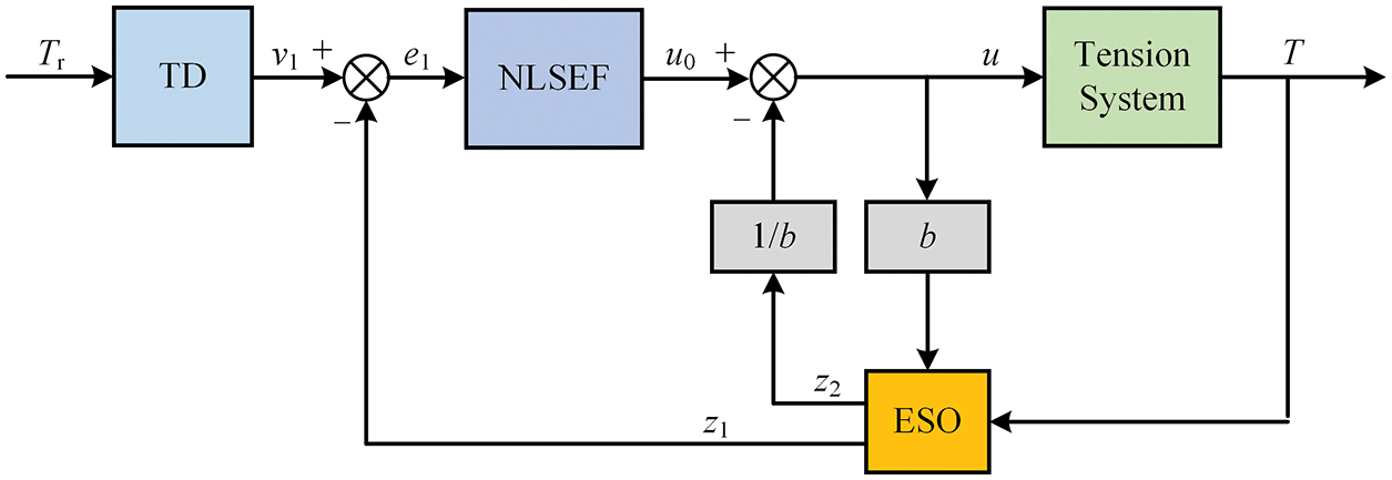
Figure 4: The structure of the ADRC controller

TD can quickly track the input signal and give its differential signal. When the input signal has a step jump, it can be used to arrange the transition process and realize the fast non-overshoot tracking of the input signal of the system. For the general second-order system, the discrete formula of TD is:

{fh(k)=fhan(v1(k)−v(k),v2(k),r,h0)v1(k+1)=v1(k)+hv2(k)v2(k+1)=v2(k)+hfh(k) (11)

where the following notations are used: v is the input signal of TD, v1 is the transition process signal, v2 is the first-order generalized differential signal of v1, h is the integral step length; h0 is the filtering factor, r is the velocity factor, and fhan (x1, x2, r, h) is the fastest control synthesis function. The specific algorithm is as follows:

{d=rh,d0=hdy=x1+hx2,a0=d2+8r|y|a={x2+(a0−d)sign(y)/2,|y|>d0x2+y/h,|y|≤d0fhan(x1,x2,r,h)=−{rsign(a),|a|>dra/d,|a|≤d (12)

The ESO is the core of ADRC which can not only track the system output variables and their differentiated signals but also actively estimate un-modeled coupling dynamics and disturbances in real time. The first-order ESO discrete algorithm can be written as:

{e(k)=z1(k)−y(k)z1(k+1)=z1(k)+h(z2(k)−β1e(k))z2(k+1)=z2(k)−hβ2fal(e(k),0.5,δ) (13)

where the following notations are used: β1 and β2 are the gain parameters of ESO, δ is the interval length of the linear segment, h is the sampling step length, and fal (e, 0.5, δ) is the function to ensure the fast and smooth convergence of ESO:

fal(e,a,δ)={(|e|asign(e),|e|>δe/δ−a,|e|≤δ (14)

NLSEF is a controller that realizes nonlinear state error feedback by the nonlinear configuration of state error. It can actively compensate for the un-modeled coupling dynamics and disturbances which are estimated by ESO in real time. The comprehensive discrete formula of NLSEF and the control law of the first-order system is as follows:

{e1(k+1)=v1(k+1)−z1(k+1)u(k+1)=knfal(e1(k+1),α,δ)−z2(k+1)/b0 (15)

where kn is the NLSEF gain coefficient, and b0 is the compensation factor. In summary, the ADRC controller combines TD, ESO, and NLSEF organically to compensate for the unknown dynamic and external disturbances of the system, and finally obtains good control performance.

According to the above steps, the design of the feedforward ADRC tension controller is completed. The feedforward controller of each span compensates for the tension velocity perturbation in advance, and superimposes the compensation with the output of the ADRC controller of each span to obtain the control quantity of this span, and finally realizes the decoupling control of tension.

3.2 Design ADRC Parameters Self-Tuning Method Based on RBF Network

The ADRC parameters tuning block diagram based on the RBF network is shown in Fig. 5. In the controller, an RBF network is set up for ESO and NLSEF, respectively. The parameter kn of NLSEF and the parameters of ESO are adjusted online at the same time. The input of the RBF network corresponding to NLSEF is system error e1, output u0 of NLSEF, and input u of tension system. The RBF network input of ESO is the output T of the tension system, the input u of the tension system, and the output estimation z1 of ESO.

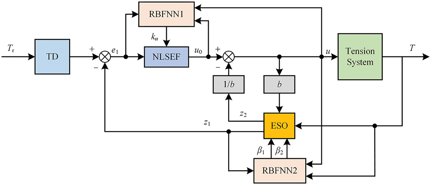
Figure 5: The structure of ADRC parameters self-tuning controller

As shown in Fig. 6, the RBF neural network structure for ADRC controller parameters tuning is 3-6-1.

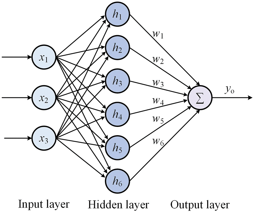
Figure 6: The structure of the RBF network

Among them, the input vector of the network is X = [x1, x2, x3], hidden layer radial basis vectors is H = [h1,h2,…, hm] 1*6. Assuming that the RBF network output is yo, and its calculation method is:

yo=wTh=w1h1+w2h2+...+wmhm,m=6 (16)

where w1~wm are the weights of different hidden layer nodes, respectively.

The radial basis function is a way to realize the nonlinear mapping from the input layer to the hidden layer. In this paper, the Gaussian function is selected as the radial basis function:

hj=exp⁡(−‖x−Cj‖22bj2),j=1,2,⋯m (17)

where Cj is the center vector of the jth node of the network, Cj = [cj1, cj2,…, cjn], and bj is the base width parameter of the node j.

In the process of training and iteration of the network, each important parameter is adjusted in real time by the gradient descent method, so that the network can identify the system state in real time by adjusting each parameter. By realizing the identification of the controlled system, the neural network model can be approximately equivalent to the system model. The specific adjustment rules are as follows:

{E1=12(y(t)−yo(t))2Δwj(t)=−η∂E1∂wj=η(y(t)−yo(t))hjwj(t)=wj(t−1)+Δwj(t)+α[wj(t−1)−wj(t−2)]Δbj=−η∂E1∂bj=η(y(t)−yo(t))wjhj‖x−Cj‖2bj3bj(t)=bj(t−1)+Δbj+α[bj(t−1)−bj(t−2)]Δcij=−η∂E1∂cij=η(y(t)−yo(t))wjhjxj−cjibj2cji(t)=cji(t−1)+Δcji+α[cji(t−1)−cji(t−2)] (18)

where E1 is the network identification performance indicator, y(t) is the output of the system, η is the network learning rate, and α is the momentum factor.

Through the RBF identification network, the adjusting strategy of ESO is to input the system output estimator z1 and the tension system output T into the RBF network at the same time, and the two variables are adjusted within the network. If there is no error between z1 and T, the adjustment of internal network parameters will be stopped; otherwise, the network parameters will be continuously trained by formula (18). The setting algorithm is used to adjust β1 and β2 until the estimator z1 realizes the estimation of the system output T. The adjustment algorithm is the negative gradient descent method, which can be written as follows:

{Δβ1(k)=η1e(k)∂y∂Δufal(e(k),α,δ)β1(k)=β1(k−1)+Δβ1(k)Δβ2(k)=η2e(k)∂y∂Δufal(e(k),α,δ)β2(k)=β2(k−1)+Δβ2(k) (19)

where η1 is the learning rate of β1, and η2 is the learning rate of β2.

The adjustment strategy of NLSEF is as follows: Continuously collect the input error e1 of the system. If e1 is not 0, the parameters of the RBF are continuously trained and adjusted by formula (18). The adjusting algorithm of NLSEF is used to adjust kn until it meets the control precision requirements of the system. The specific algorithm is shown as:

{Δkn(k)=η3e1(k)∂y∂Δufal(e1(k),α,δ)kn(k)=kn(k−1)+Δkn(k) (20)

where η3 is the learning rate of β3.

3.3 Design Tension Observer for Dancer Roll

It can be known from Section 2.1 that the principle of dancer roll is to obtain the deflection angle of the dancer roll by the sensors, and the fluctuation of the substrate tension can be obtained by using the mathematical model of the dancer roll in formula (2). According to the formula, to obtain the actual substrate tension, the first-order and second-order derivatives of the angle signal must be solved, and then the two derivative results are substituted into the mathematical model, which inevitably leads to serious amplification of the disturbance signal, and also makes it difficult to ensure the real-time performance during operation. Therefore, we take advantage of the good filtering properties of ESO, add ESO into the dancer roll tension detection link, and design a dancer roll tension observer based on ESO to achieve high precision detection of the tension system. The structure of the tension observer is shown in Fig. 7.

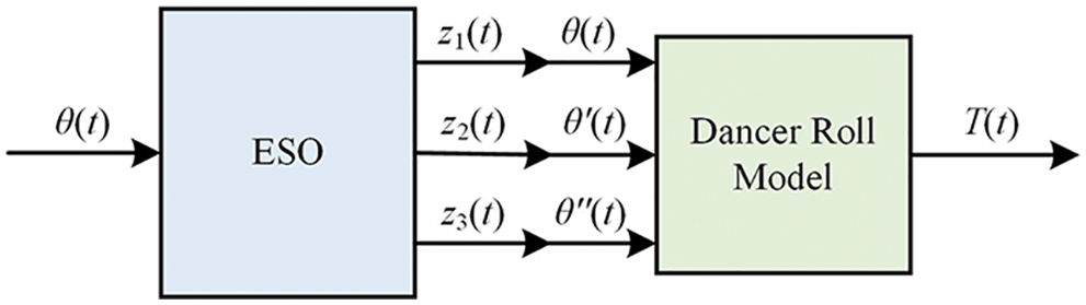
Figure 7: The structure of tension observer

Where the following notations are used: θ(t) is the deflection angle of dancer roll, z1(t) is the tracking signal of θ(t), z2(t) is the first-order derivative estimator of θ(t), and z3(t) is the second-order derivative estimator of θ(t). In the tension observer, after receiving the dancer roll deflection angle θ(t), ESO calculates z1(t), z2(t), and z3(t), respectively, and replaces θ(t), θ′(t), and θ″(t) with the obtained z1(t), z2(t) and z3(t). Then the three values are substituted into the mathematical model of the dancer roll to calculate the tension value T(t) of the substrate. In this process, ESO will filter the high-order interference signal when the sensors measure the deflection angle of dancer roll, greatly reducing the original high-order interference and making the measurement of the substrate tension for the dancer roll more accurate.

Since the dancer roll model is a second-order system, it is necessary to use the second-order ESO to design the tension observer. The discrete calculation formula of the second-order ESO is:

{e(k)=z1(k)−y(k)z1(k+1)=z1(k)+h(z2(k)−β1e(k))z2(k+1)=z2(k)+h(z3(k)−β2fal(e(k),0.5,δ)+b0u(k))z3(k+1)=z3(k)−hβ3fal(e(k),0.25,δ) (21)

According to the ESO algorithm in formulas (2) and (21), the discrete formula of the tension observer can be obtained as follows:

{e(k)=z1(k)−θ(k)z1(k+1)=z1(k)+h(z2(k)−β1e(k))z2(k+1)=z2(k)+h(z3(k)−β2fal(e(k),0.5,δ))z3(k+1)=z3(k)−hβ3fal(e(k),0.25,δ)T(k)=12l2{−Jeqz3(k)−beqz2(k)+l1[FP1−kl1z1(k)]} (22)

Based on the above steps, the design of the dancer roll tension observer is realized.

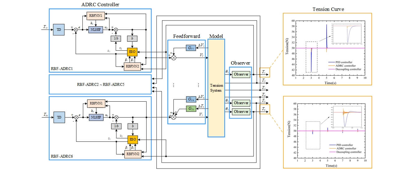
3.4 Design Feedforward Decoupling Controller Based on RBF-ADRC

Combined with the above research, a feedforward ADRC parameters self-tuning decoupling controller based on RBF network is designed in this section, the structure is shown in Fig. 8, in which only the controller’s structure of the first and last tension span are given in detail, and the rest parts are omitted. The overall structure of the designed controller is mainly composed of three parts: 1. RBF-ADRC controller. It mainly consists of 6 RBF-ADRC controllers from different tension spans. According to the specific ADRC controller parameters tuning algorithm, the tuned parameters are transmitted to ADRC in real time, and then ADRC outputs the main loop control quantity. 2. Feedforward controller. This part compensates for the velocity and tension disturbance of each span in advance, and realizes the decoupling control for the system. 3. Tension observer. By using the designed tension measurement method in Section 3.3, the conversion from the offset angle θ of the dancer roll to the tension value T of the substrate is realized.

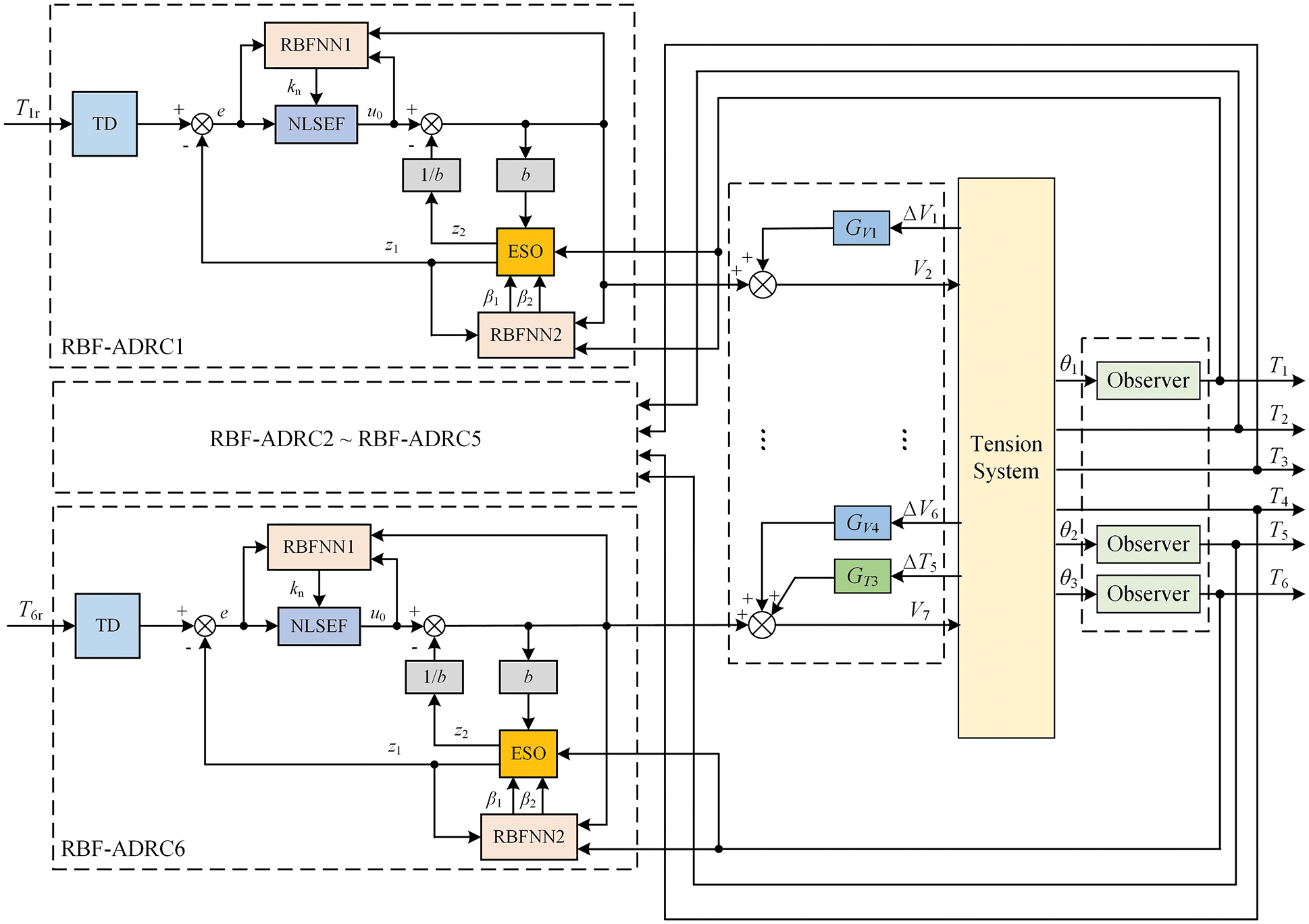
Figure 8: The overall structure of the controller

The RBF-ADRC controller for each tension span is the core part of the feedforward ADRC parameters self-tuning decoupling controller based on the RBF network designed in this section. It includes a TD, an ESO, a NLSEF, and an RBF network designed for ESO and NLSEF, respectively. TD is responsible for arranging the transition process to solve the unreasonable error extraction problem existing in the ordinary PID control and avoid the system overshoot in the control process. ESO can realize the tracking of output variables and estimation of external disturbances. Since the traditional PID control is a linear combination of the proportional part, the integral part, and the differential part, it may not be able to show good results when controlling the nonlinear system. NLSEF is a nonlinear combinatorial method that is used to achieve a reasonable combination of errors and differential errors and to actively compensate for the total disturbance of the system using the control law with ESO together. Two RBF neural networks are responsible for real-time adjustment of ESO and NLSEF parameters respectively. Through these steps, the outputs of the RBF-ADRC controllers are obtained and then transmitted to the mathematical model of the tension system. Finally, the control amount of the tension span can be obtained after adding the output of the feedforward controller.

4  Simulation and Analysis for the Designed Controller

In order to verify and analyze the performance of the designed feedforward ADRC parameters self-tuning decoupling controller based on RBF network, the tension observer part and the tension controller part are simulated respectively based on MATLAB.

4.1 Simulation and Analysis of Tension Observer

The mathematical model of the dancer roll is built by using the Simulink module in MATLAB. In one case, input directly the angle signal fluctuation into the mathematical model of the dancer roll to calculate the substrate tension. In the other case, the angle signal is input to the tension observer, and the output of the tension observer is calculated to get the substrate tension. The tension fluctuation curves under the two conditions are compared.

In the simulation, the steady tension value of the dancer roll is set as 50N, and the simulation time is set as 30 s. First, the dancer roll is made to produce an angular step of 0.01 at the 5th s of system operation; Second, the dancer roll is made to continuously produce random fluctuations of ±0.01. The simulation results of ordinary dancer roll are shown in Fig. 9, and the simulation results of the ESO-based dancer roll tension observer are shown in Fig. 10.

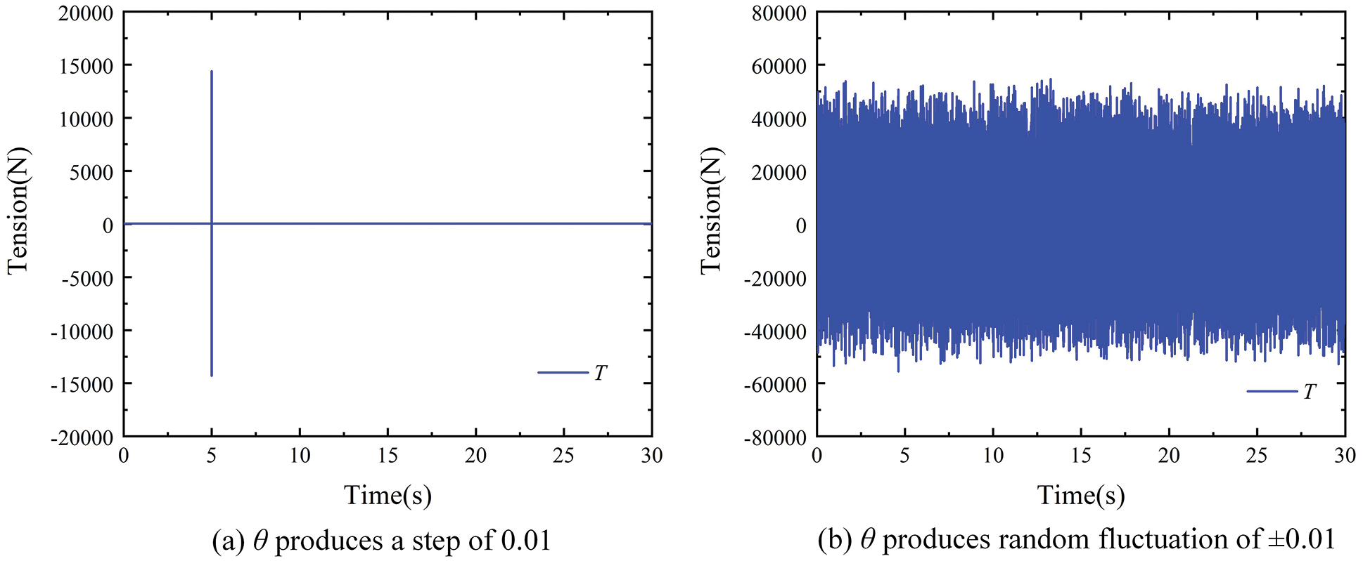
Figure 9: Simulation results of the ordinary dancer roll

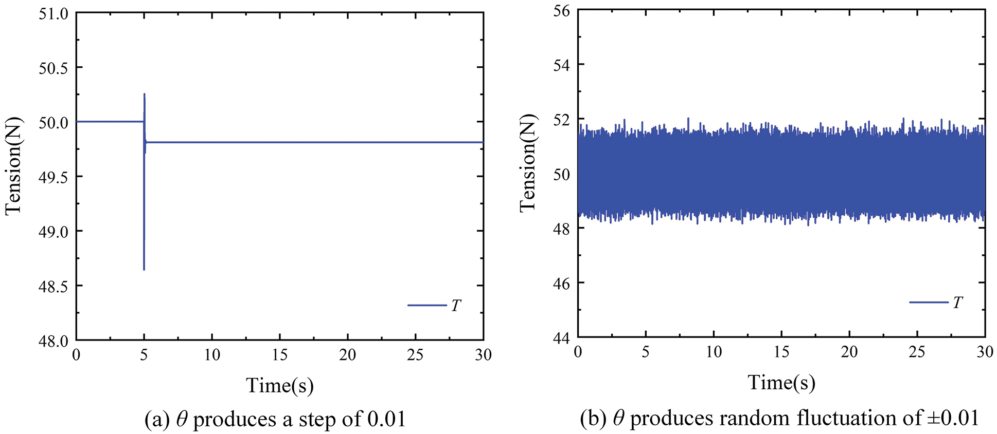
Figure 10: Simulation results of the ESO-based dancer roll

By comparing the simulation results of the two groups, the disturbance amplification effect is obvious when the deflection angle θ of the dancer roll changes without the tension observer. When θ produces a step of 0.01, the tension output T has a sudden change of ±15000N, and when θ produces a random fluctuation of ±0.01, the tension output T generates a disturbance of ±50000N. In contrast, when the designed tension observer is used, the tension output T changes from 48.6N to 50.25N when θ produces a step of 0.01, and the tension output T fluctuates from 48.5N to 52N when θ produces a ±0.01 random fluctuation. Therefore, the tension observer based on ESO designed in this paper can effectively solve the problem of serious amplification of interference by the second-order differential link of dancer roll model. It realizes the filtering effect on the interference signal, and measures tension value more accurate and stable.

4.2 Simulation and Analysis of Feedforward Decoupling Controller Based on RBF-ADRC

To verify the performance of the proposed feedforward ADRC parameters self-tuning decoupling controller, the designed controller model is simulated and compared with the control results of the tension system under PID and ADRC controllers. As shown in Table 1, the model parameters used in the simulation are taken from the actual roll-to-roll precision coating machine.

During the simulation, the steady-state tension value of the system is set as 50N, and the synchronization velocity of the system is set as 150 m/min and 300 m/min to represent the system operation under different working conditions. The number of nodes in the hidden layer of the RBF neural network is set as 6, and the program code is written in the S-function module in Simulink. The parameters of each RBF-ADRC controller are shown in Table 2, where ηE and ηN are the RBF network identification rates designed for ESO and NLSEF respectively. The parameters of each PID and ADRC controller are shown in Tables 3 and 4.

In addition to the parameters noted in Table 2, other parameters include the following matrices, which are consistent across all RBF-ADRC controllers for the matrix type.

cj=[303030303030303030303030],bj=[404040404040],ωj=[101010101010],hj=[111111],j=0,1,...,6 (23)

4.2.1 Simulation Analysis of Tension Decoupling

In the tension system of the roll-to-roll precision coating machine, the tension output of each span is taken as input into the next span, and there is a serious coupling relationship between the tension of each span. If the tension fluctuation occurs during the normal operation of the equipment, that tension fluctuation will also be transmitted backward with the operation of the substrate. It means that the tension fluctuation of a span in the system will cause the tension fluctuation of multiple spans at the same time. Therefore, when analyzing the decoupling performance of the decoupling controller through simulation, it is necessary to apply changes to the tension of different spans at different times, to illustrate the decoupling effect of the controller.

The simulation conditions of this part are as follows: After the tension system is stabilized, T1, T2, and T3 are made to generate respectively a tension pulse with a value of 1N and a duration of 1s at the 2nd, 5th, and 8th s. Under different working conditions (150 m/min and 300 m/min of substrate speed), the tension decoupling curves with different controllers are shown in Figs. 11 and 12, as well as the designed controller ESO parameter adjustment curves are shown in Figs. 13 and 14, and the NLSEF parameter adjustment curves are shown in Figs. 15 and 16.

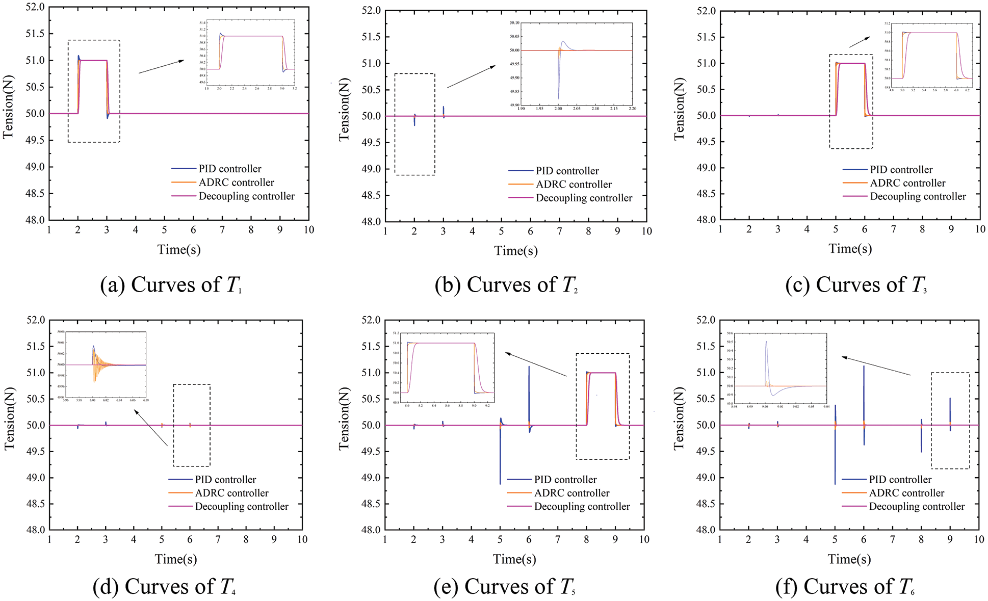
Figure 11: Tension decoupling curves when substrate velocity is 150 m/min

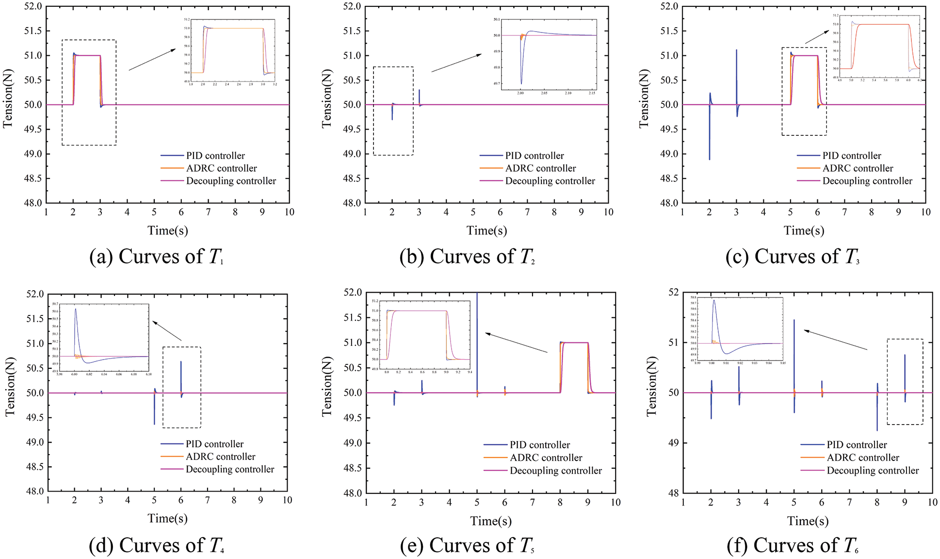
Figure 12: Tension decoupling curves when substrate velocity is 300 m/min

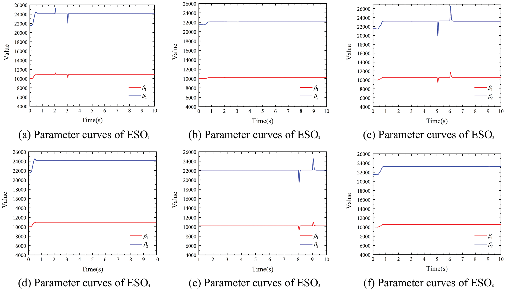
Figure 13: ESO parameter adjustment curves under tension disturbance (150 m/min)

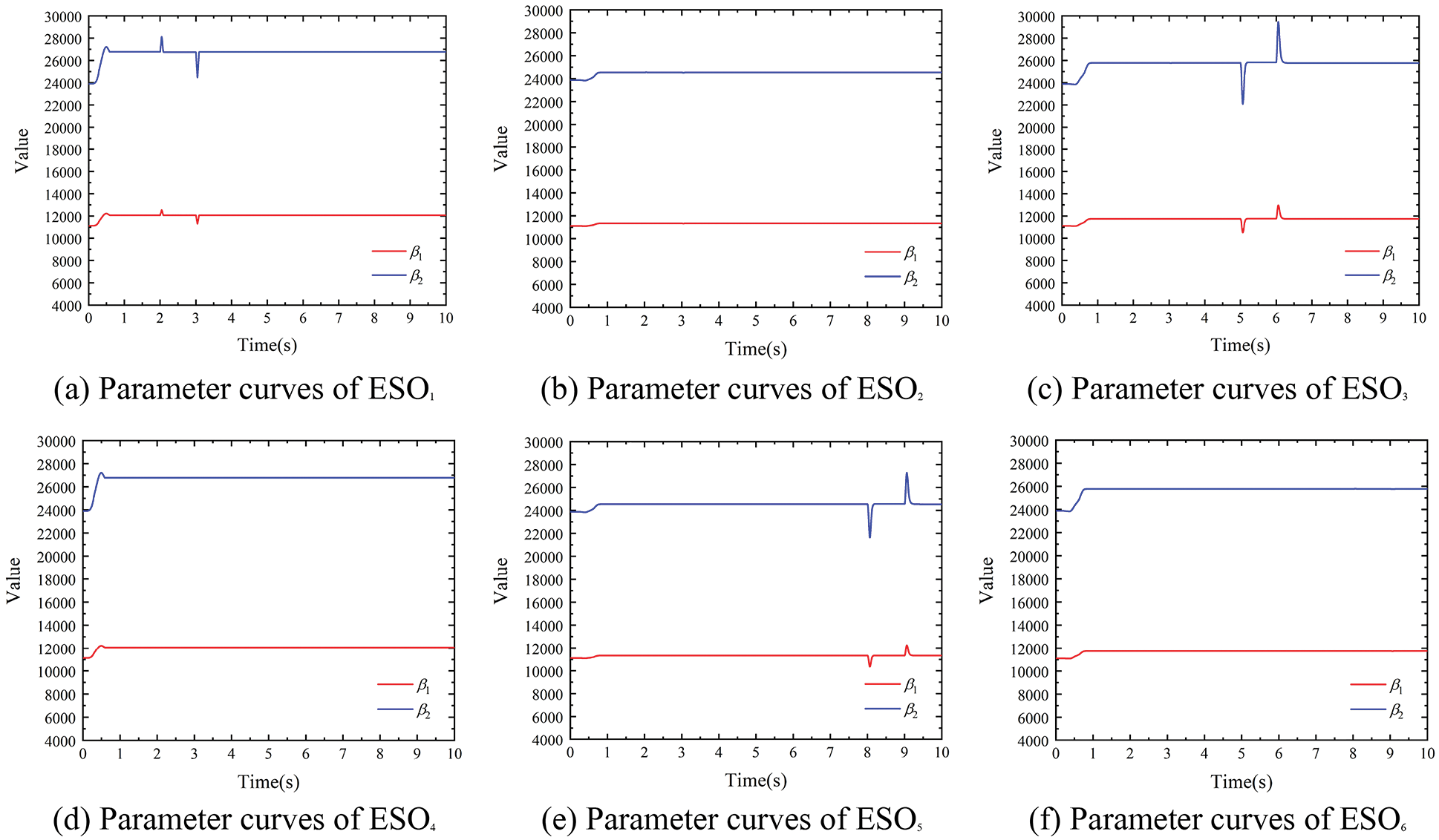
Figure 14: ESO parameter adjustment curves under tension disturbance (300 m/min)

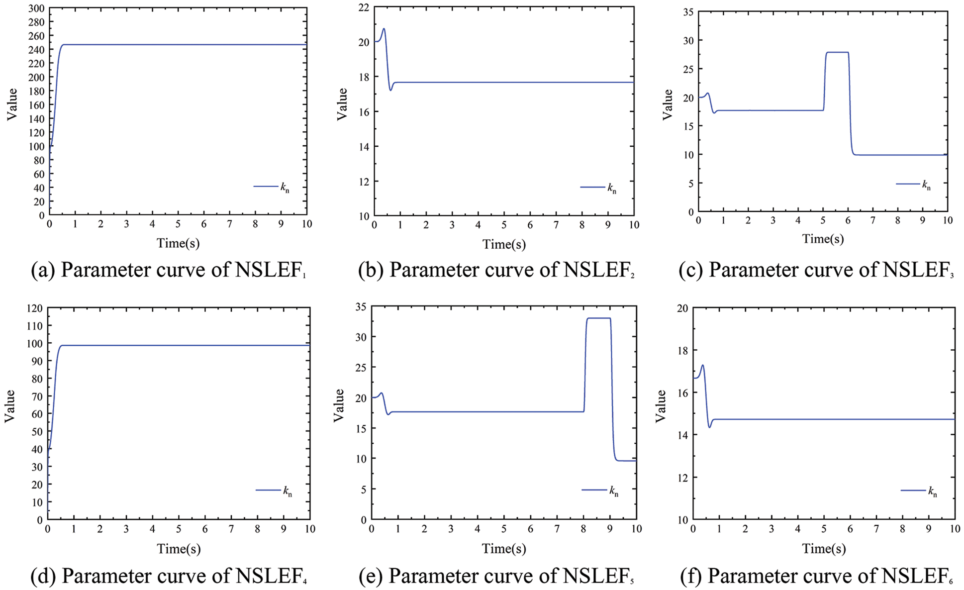
Figure 15: NSLEF parameter adjustment curves under tension disturbance (150 m/min)

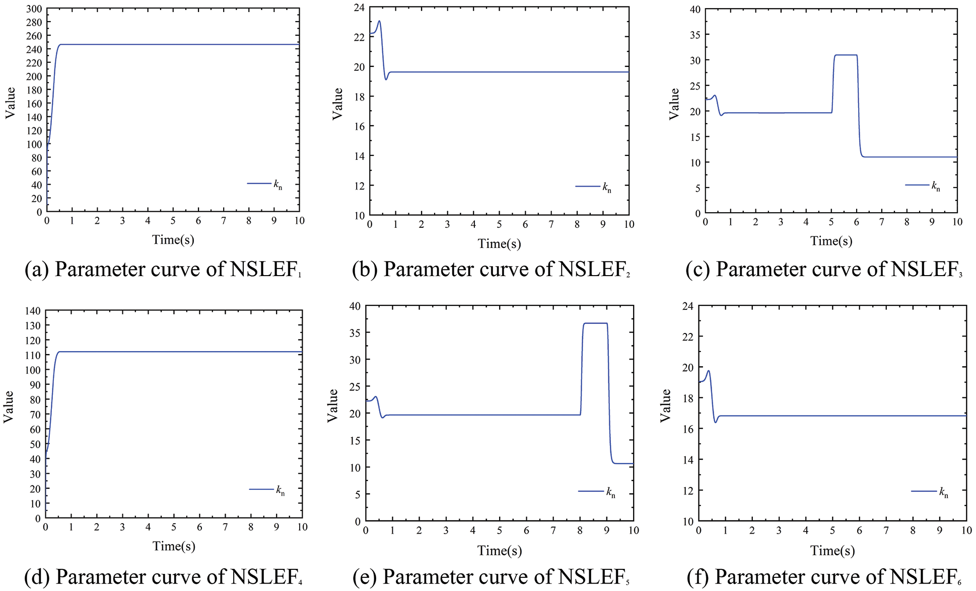
Figure 16: NSLEF parameter adjustment curves under tension disturbance (300 m/min)

According to the simulation results, it can be seen that when using the traditional PID for tension system control, the change of tension pulse generated by the substrate tension at different times will cause tension fluctuations in the subsequent span, and its steady-state tension amplitude range fluctuates more. When the conventional ADRC controller controls the tension system, its steady-state tension fluctuation amplitude range is much smaller than the steady-state tension fluctuation amplitude range in PID control. While the designed decoupling controller obviously shows better control performance than the former two controllers in both working conditions, and its steady-state tension fluctuation amplitude range is basically 0N.

In Figs. 11 and 12, when using the PID and ADRC controllers, respectively, the tension pulses generated by T1, T3, and T5 all cause obvious fluctuation of the subsequent tension spans, while the decoupling controller can realize the decoupling control when the tension pulse is generated. At the same time, the RBF network of the decoupling controller can adjust ESO and NLSEF parameters in real time when the stable state of the system changes. The simulation results show that the designed decoupling controller can realize the decoupling control when the tension of each span fluctuates, which verifies the tension decoupling performance of the controllers.

4.2.2 Simulation Analysis of Velocity Decoupling

In addition to the coupling effect of tension between different spans, the velocity of each motor is also a very important coupling quantity in the tension system. Taking the infeeding motor as an example, in the stable state of the system, the sudden change of V2 means that both the control quantity of unwinding span and the interference quantity of infeeding span change, which will cause tension fluctuation of both T1 and T2. Additionally, due to the propagation characteristics of tension, the tension fluctuation generated by T1 and T2 will also cause the fluctuation of T3~T6, other motor velocities also show the same characteristics. It is obvious that the coupling effect between each motor velocity has an important influence on the decoupling control of the tension system, and the velocity decoupling performance of the controller needs to be analyzed through simulation.

The simulation conditions of this part are as follows: After the system is stabilized, V1 is made to produce a velocity step of 6 m/min at the 3rd s. V1 is made to produce a velocity step of −6 m/min at the 5th s. V4 is made to produce a velocity step of 3 m/min at the 7th s. V4 is made to produce a velocity step of −3 m/min at the 9th s. Under different working conditions (150 m/min and 300 m/min of substrate speed), the tension decoupling curves with different controllers are shown in Figs. 17 and 18, as well as the designed controller ESO parameter adjustment curves are shown in Figs. 19 and 20, and the NLSEF parameter adjustment curves are shown in Figs. 21 and 22.

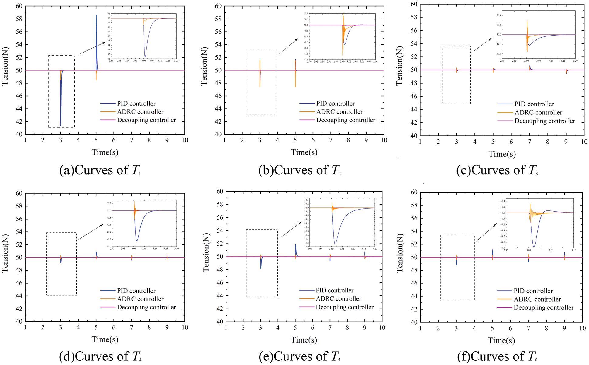
Figure 17: Velocity decoupling curves when substrate velocity is 150 m/min

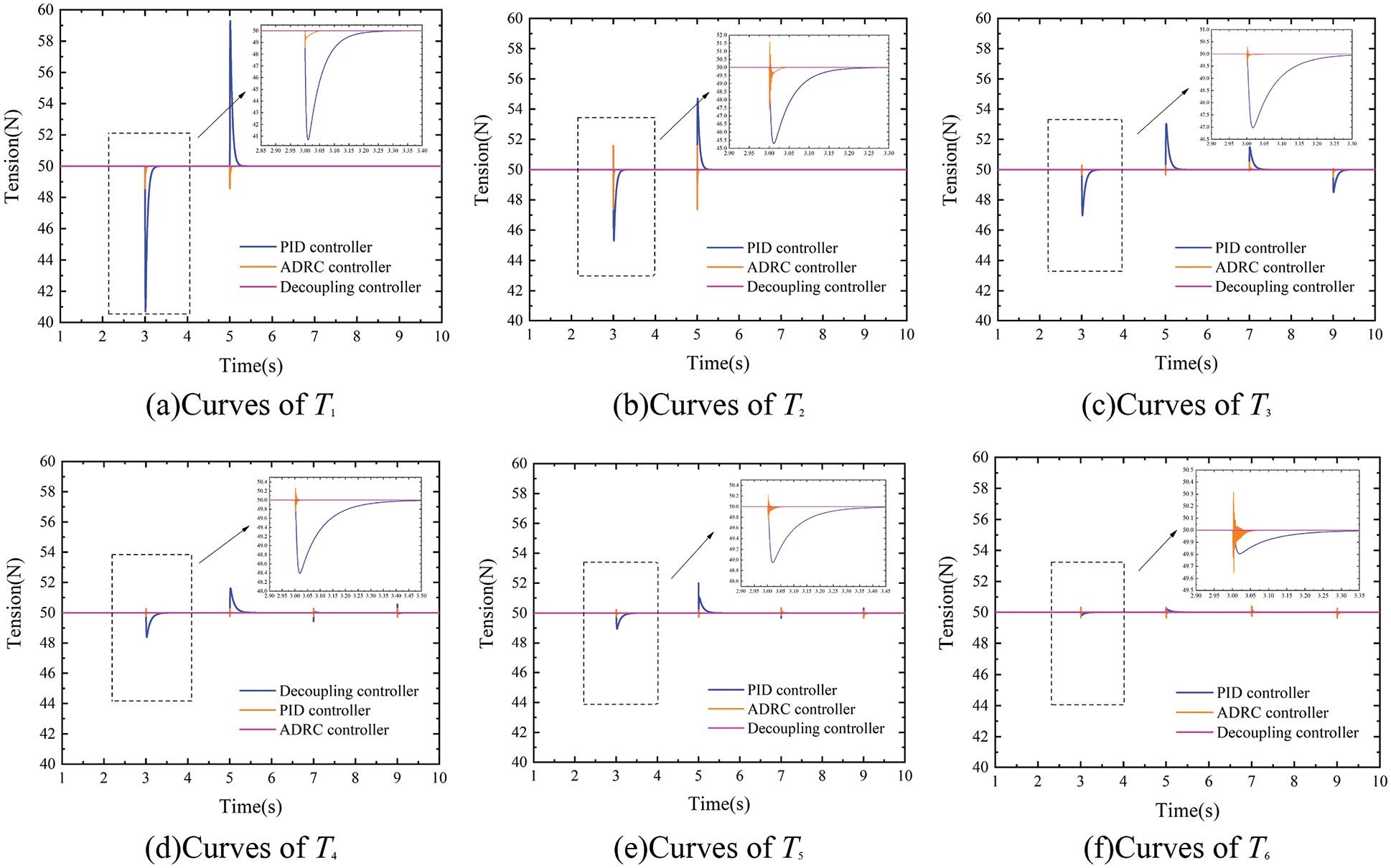
Figure 18: Velocity decoupling curves when substrate velocity is 300 m/min

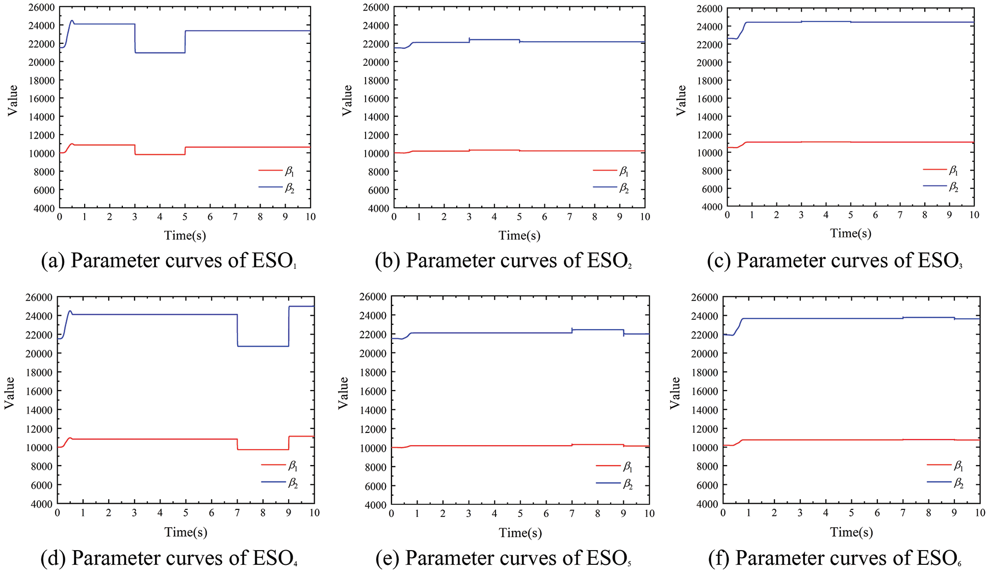
Figure 19: ESO parameter adjustment curves under velocity disturbances (150 m/min)

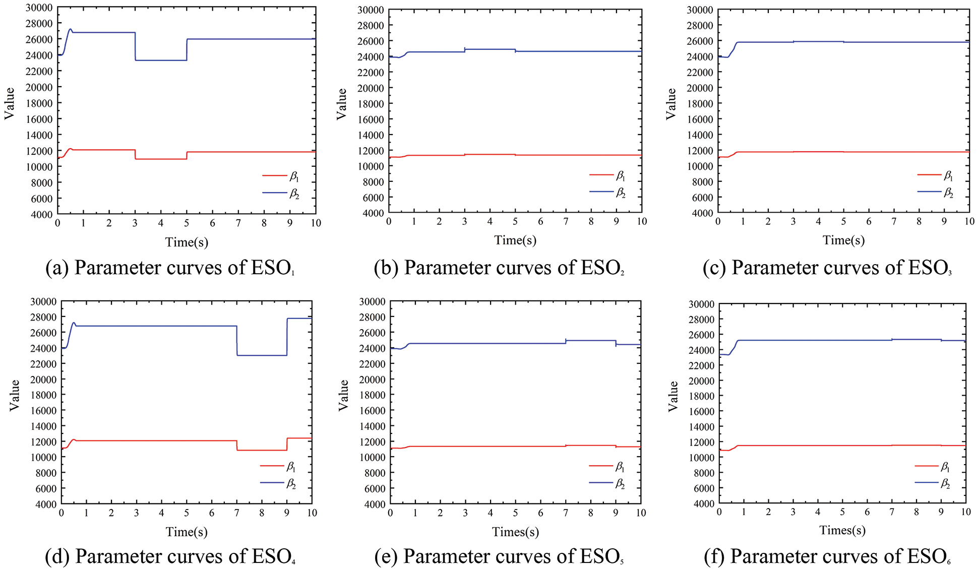
Figure 20: ESO parameter adjustment curves under velocity disturbances (300 m/min)

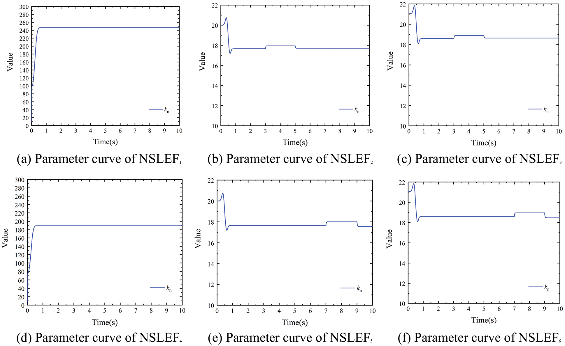
Figure 21: NLSEF parameter adjustment curves under velocity disturbance (150 m/min)

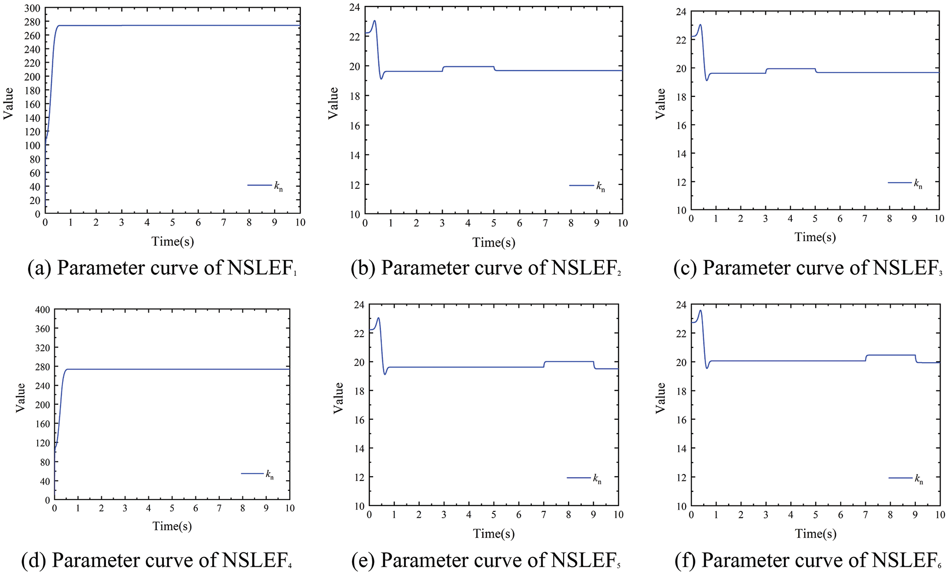
Figure 22: NLSEF parameter adjustment curves under velocity disturbance (300 m/min)

As can be seen from Figs. 17 and 18, when the tension system is controlled by traditional PID and ADRC controllers respectively, the maximum tension fluctuation is ±10N and ±1N, respectively. The change of velocity will cause fluctuations of the substrate tension in the two adjacent front and back spans, and this tension fluctuation will propagate backward with the movement of the substrate, so that multiple tension units will be affected. On the contrary, the designed decoupling controller can compensate for the tension fluctuation caused by the speed change in advance, which makes the tension fluctuation almost 0N.

As is shown, when PID and ADRC control are adopted respectively, the velocity step change generated by V1 leads to obvious fluctuation of substrate tension of all spans from T1 to T6, and the velocity step change generated by V4 leads to the change of tension from T3 to T6. While with the decoupled controller, the change of velocity does not affect tension of each span, and the decoupling control effect of each tension span is realized when the change of velocity occurs. In addition, the designed controller also realized the effect of online adjustment of ADRC parameters. The simulation results show that the designed controller also has good control ability to deal with the tension fluctuation caused by the velocity change, and realizes decoupling control of the velocity.

5  Conclusion

Control accuracy of tension system is an important index to evaluate the performance of roll-to-roll precision coating machine. In order to improve the control accuracy of tension system, this paper proposes an ADRC parameters self-tuning decoupling control strategy based on feedforward control, ADRC and RBF neural network for the coating machine. The strategy is unique in which it uses feedforward controllers to compensate for the tension fluctuation caused by the modeled interferences, ADRC controllers to adjust the inputs of the tension system, and the RBF neural network to realize the self-tuning of ADRC parameters in real time. In addition, a tension observer is designed based on ESO to solve the problem of amplification interference during the tension measurement of dancer roll, and the simulation results show that the tension observer can effectively filter out the interference in the tension measurement process. To evaluate the performance of the proposed decoupling strategy, simulations and comparative analysis among PID, ADRC and proposed decoupling controllers are carried out by MATLAB. The simulation results illustrate that the proposed strategy has a good decoupling control effect and realizes the online adjustment of ADRC parameters, and it also shows excellent dynamic performance. In the future, the designed controller will be further experimented with algorithms and launched for applications on actual coating machines as well as other roll-to-roll equipment.

Funding Statement: This project is supported by the National Key Research and Development Program of China (Grant No. 2019YFB1707200), the Key Research and Development Program of Shaanxi Province (Grant No. 2020ZDLGY14-06), the Technology Innovation Leading Program of Shaanxi Province (Grant No. 2020QFY03-03).

Conflicts of Interest: The authors declare that they have no conflicts of interest to report regarding the present study.

References

1. Xiao, Y. J., Zhang, Z. P., Liu, Z. H., Liu, W. L., Gao, N. et al. (2022). Optimal analysis and application of the warp tension control system for a rapier loom. Textile Research Journal, 92(7), 1213–1225. DOI 10.1177/00405175211053662. [Google Scholar] [CrossRef]
2. Zhang, H. J., Tang, H., Shi, Y. Y. (2018). Precision tension control technology of composite fiber tape winding molding. Journal of Thermoplastic Composite Materials, 31(7), 925–945. DOI 10.1177/0892705717729018. [Google Scholar] [CrossRef]
3. Seki, K., Kikuchi, T., Iwasaki, M. (2020). Tension controller design considering periodic disturbance suppression in roll-to-roll web handling systems. IEEJ Journal of Industry Applications, 9(1), 36–42. DOI 10.1541/ieejjia.9.36. [Google Scholar] [CrossRef]
4. Huang, H. X., Xu, J. Z., Sun, K. W., Deng, L. W., Huang, C. (2020). Design and analysis of tension control system for transformer insulation layer winding. IEEE Access, 8, 95068–95081. DOI 10.1109/ACCESS.2020.2995591. [Google Scholar] [CrossRef]
5. Jiang, C., Wang, H. S., Hou, L. W., Jiang, L. L. (2019). Sliding mode compensation control for diaphragm tension in unwinding process of lithium battery diaphragm slitting machine. IEEE Access, 8, 21302–21313. DOI 10.1109/ACCESS.2019.2945976. [Google Scholar] [CrossRef]
6. Chen, J., Hou, H. L., Yang, T. G. (2019). Robust decentralized H∞ control for a multi-motor web-winding system. IEEE Access, 7, 41241–41249. DOI 10.1109/ACCESS.2019.2906223. [Google Scholar] [CrossRef]
7. Kuznetsov, B., Nikitina, T., Bovdui, I., Kobilyanskiy, B. (2019). Robust anisotropic control by cable winding machine. 2019 IEEE International Conference on Modern Electrical and Energy Systems, 2019, 38–41. DOI 10.1109/MEES.2019.8896651. [Google Scholar] [CrossRef]
8. Liu, L., Shao, N., Lin, M. H., Fang, Y. M. (2019). Hamilton-based adaptive robust control for the speed and tension system of reversible cold strip rolling mill. International Journal of Adaptive Control and Signal Processing, 33(4), 626–643. DOI 10.1002/acs.2977. [Google Scholar] [CrossRef]
9. Talian, P., Perdukova, D., Fedor, P. (2018). Stable and robust tension controller for middle section of continuous line. Elektronika ir Elektrotechnika, 24(1), 3–10. DOI 10.5755/j01.eie.24.1.20148. [Google Scholar] [CrossRef]
10. Liu, S. H., Yin, B. Z., Ma, L., Xu, H. W., Zhu, G. S. (2016). A decoupling control strategy for multilayer register system in printed electronic equipment. Mathematical Problems in Engineering, 2016(6), 1–14, 7165163. DOI 10.1155/2016/7165163. [Google Scholar] [CrossRef]
11. Khaled, T. A., Akhrif, O., Bonev, I. A. (2020). Dynamic path correction of an industrial robot using a distance sensor and an ADRC controller. IEEE/ASME Transactions on Mechatronics, 26(3), 1646–1656. DOI 10.1109/TMECH.2020.3026994. [Google Scholar] [CrossRef]
12. Hai, X. S., Wang, Z. L., Feng, Q., Ren, Y., Xu, B. H. et al. (2019). Mobile robot ADRC with an automatic parameter tuning mechanism via modified pigeon-inspired optimization. IEEE/ASME Transactions on Mechatronics, 24(6), 2616–2626. DOI 10.1109/TMECH.2019.2953239. [Google Scholar] [CrossRef]
13. Hezzi, A., Ben, E. S., Bensalem, Y., Zhou, Z., Benbouzid, M. et al. (2020). Adrc-based robust and resilient control of a 5-phase pmsm driven electric vehicle. Machines, 8(2), 17. DOI 10.3390/machines8020017. [Google Scholar] [CrossRef]
14. Ding, M., Zhao, S. H. (2020). Tension control of unwinding system based on seeker optimization auto disturbance rejection control. Wool Textile Journal, 48(1), 85–91. DOI 10.19333/j.mfkj.20190403707. [Google Scholar] [CrossRef]
15. Liu, S. H., Mei, X. S., Kong, F. F., He, K., Zhu, G. S. (2013). A decoupling control algorithm for unwinding tension system based on active disturbance rejection control. Mathematical Problems in Engineering, 2013, 1–18, 439797. DOI 10.1155/2013/439797. [Google Scholar] [CrossRef]
16. Wang, Z. Y., Liu, S. H., He, K., Shi, W. L., Chen, S. W. (2020). Design decoupling controller for rewinding system of the gravure printing machines. Information Technology and Mechatronics Engineering Conference, pp. 908–912. DOI 10.1109/ITOEC49072.2020.9141756. [Google Scholar] [CrossRef]
17. Zhang, D. Y., Wu, Q. H., Yao, X. L., Jiao, L. L. (2018). Active disturbance rejection control for looper tension of stainless steel strip processing line. Journal of Control Engineering and Applied Informatics, 20(4), 60–68. [Google Scholar]
18. Yin, J., Wang, R., Gao, Q., Zhang, W. (2019). Fractional order PID of AC servo system based on neural network active disturbance rejection control. Electronics Optics & Control, 26(5), 20–25. [Google Scholar]
19. Kumar, R., Agrawal, H. P., Shah, A., Bansal, O. B. (2019). Maximum power point tracking in wind energy conversion system using radial basis function based neural network control strategy. Sustainable Energy Technologies and Assessments, 36, 100533. DOI 10.1016/j.seta.2019.100533. [Google Scholar] [CrossRef]
20. Li, M., Feng, H., Zhang, Y. (2018). RBF neural network tuning PID control based on UMAC. Journal of Beijing University of Aeronautics and Astronautics, 44(10), 2063–2070. DOI 10.13700/j.bh.1001-5965.2017.0777. [Google Scholar] [CrossRef]
21. Kang, H., Shin, K. H. (2018). Precise tension control of a dancer with a reduced-order observer for roll-to-roll manufacturing systems. Mechanism and Machine Theory, 122(3), 75–85. DOI 10.1016/j.mechmachtheory.2017.12.012. [Google Scholar] [CrossRef]
22. Wang, Z. Y., Liu, S. H., Feng, L., Zhang, Z. Q., Liu, J. Q. (2022). Coupling modeling and analysis of the tension system for roll-to-roll gravure printing machines. Journal of Imaging Science and Technology, 66(2), 020401-1–020401-10. DOI 10.2352/J.ImagingSci.Technol.2022.66.2.020401. [Google Scholar] [CrossRef]
23. Wang, Z. Y., Liu, S. H., Jiao, F. Q., Zhang, Z. Q., Chen, W. F. (2021). Design tension controller for the rewinding system of roll-to-roll precision coating machine. Advanced Information Management, Communicates, Electronic and Automation Control Conference, 4, 1156–1160. DOI 10.1109/IMCEC51613.2021.9482045. [Google Scholar] [CrossRef]
24. Zhang, M. Y., Li, Q. D. (2022). A compound scheme based on improved ADRC and nonlinear compensation for electromechanical actuator. Actuators, 11(3), 93. DOI 10.3390/act11030093. [Google Scholar] [CrossRef]
Cite This Article
Copyright © 2023 The Author(s). Published by Tech Science Press.
This work is licensed under a Creative Commons Attribution 4.0 International License , which permits unrestricted use, distribution, and reproduction in any medium, provided the original work is properly cited.
Downloads
Citation Tools