Genetic Diversity and Population Structure Analysis of Barley Landraces from Shanghai Region Using Genotyping-by-Sequencing

1  Introduction

Barley, one of the earliest crops to be domesticated by humans, is the fourth most important cereal crop in the world nowadays because of its wide range of uses, including brewing, animal feed and human consumption [1]. It is widely cultivated on all continents except Antarctica because of its good adaptability. Barley is also used as a model plant for the Triticeae tribe because of its diploid characteristics [2,3]. However, modern barley cultivars, like other crops, are suffering problems caused by narrowed genetic backgrounds, and these problems are aggravated by climate change and frequent extreme weather events [4–7]. Thus, it is necessary to collect and utilize more barley germplasms to meet the requirements of barley breeding in the future.

Barley landraces, as for most crops, are less inbred and have more genetic diversity than modern varieties [1]. They have a long planting history and good adaptations to certain locations mainly based on harboring many biotic and abiotic stress resistance genes. However, mistakes in naming some landraces and duplications of genotypes have often occurred during the collection of landrace resources because landraces were maintained mainly by local farmers over generations. This is true of the Shanghai region in China where there has been a long tradition of barley cultivation and many barley landraces have been handed down [8]. Therefore, it is necessary to know the genetic backgrounds of these landraces for name correction, duplicate removal, conservation and barley improvement.

Although the genetic diversity of barley landraces in the Shanghai region has previously been analyzed using simple sequence repeat (SSR) markers, many genotypes were still not well differentiated due to the lack of available markers or low polymorphism [8]. With the development of sequencing technology, the genotyping-by-sequencing (GBS) approach has been developed for genetic diversity analysis, with high polymorphism and low cost [9–11]. It has been used in many crops, such as rice [12], wheat [13] and maize [14], and there has also been representative work in a barley collection [15]. In the present study, genetic diversity and population structure analyses of a collection of 112 barley landraces from the Shanghai region were conducted using GBS. The aims of this study were to evaluate the genetic diversity and ancestral origins of the barley landraces from the Shanghai region and reveal the effects of the two morphological traits of row-type and adherence of hulls on the formation of barley landraces.

2  Materials and Methods

2.1 Plant Materials and DNA Extraction

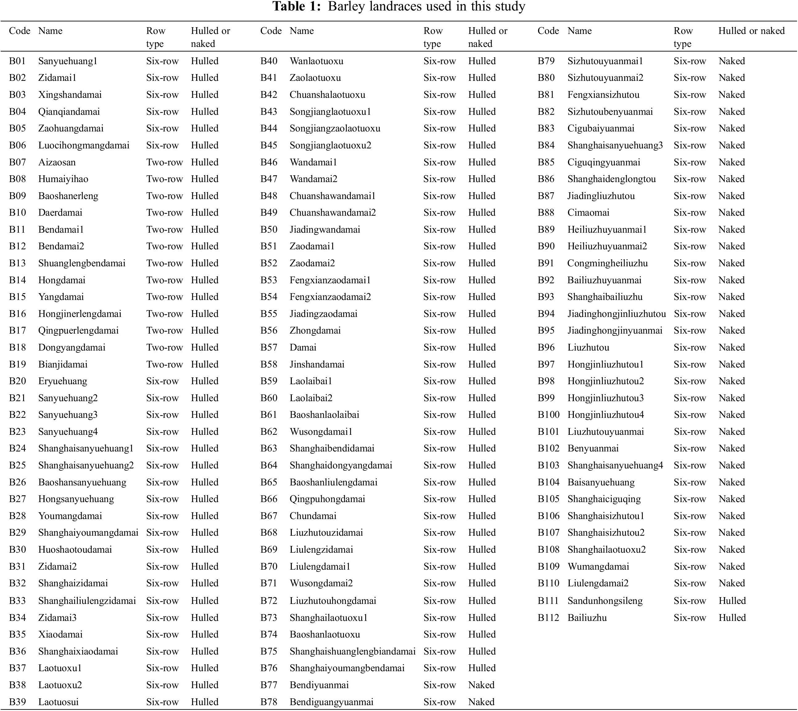
A collection of 112 barley landraces from the Shanghai region of China was used in this study (Table 1) [8]. These barley landraces, which were originally obtained from Shanghai Agrobiological Gene Center and propagated and preserved at Shanghai Academy of Agricultural Sciences, comprised 13 two-rowed and hulled landraces, 65 six-rowed and hulled landraces, and 34 six-rowed and naked landraces.

Seeds of each landrace were sown in seedling trays in an artificial climate room at Shanghai Academy of Agricultural Sciences in China. Leaves were sampled at the three-leaf stage, then quickly frozen in liquid nitrogen and stored at −80°C. Genomic DNA was extracted using a DNA Secure Plant Kit (Tiangen) according to the manufacturer’s instructions. DNA degradation and contamination were assessed by electrophoresis through a 1% agarose gel; purity and concentration were measured using a NanoDrop 2000 Spectrophotometer (Thermo Fisher Scientific, Wilmington, USA).

2.2 GBS Library Construction, Nucleotide Sequencing and SNP Calling

Genomic DNA (200 ng) was digested with PstI-HF and MspI (New England Biolabs, Ipswich, UK) and processed for GBS library construction according to Qi et al. [11]. Then, the DNA fragments were ligated using T4 DNA ligase (New England Biolabs, Ipswich, UK), and fragments smaller than 300 bp were removed. The ligated DNA fragments were amplified by PCR for preparing GBS libraries. The PCR products were checked by electrophoresis through a 1.5% agarose gel and the DNA concentration was measured using a Qubit 2.0© fluorometer and a Qubit™ dsDNA HS assay kit. GBS libraries with DNA concentrations >5.0 ng/μL were taken for nucleotide sequence analysis on the Illumina Nova platform (Illumina Inc., San Diego, USA) and 150 bp pair-end reads were generated. The clean data ranged from 1.24 to 1.77 Gb, and Q30 percentages were all >88% (Table S1).

The Single Nucleotide Polymorphisms (SNPs) were called by using Genome Analysis Tool Kit (GATK) software (v4.1.3) with the model of Haplotype caller [16]. The barley reference genome downloaded from Ensembl Plants (http://plants.ensembl.org/Hordeum_vulgare/Info/Index, IBSC v2) was used for the SNP calling. Three criteria were applied for SNP filtering using VCFtools (v0.1.16) [17]: (1) Loci with sequencing depth ⩾4 were retained; (2) Loci with minor allele frequency (MAF) <0.01 were discarded; (3) Loci that were missing in more than 20% of the samples were excluded. The filtered SNPs were annotated by using SnpEff (v4.1g) [18].

2.3 Genetic Diversity Analysis

For genetic diversity analysis, genetic parameters such as Hardy-Weinberg equilibrium P-value (HW-P) and nucleotide diversity (π) were calculated for each SNP marker using VCFtools (v0.1.16). The expected heterozygosity (He) was calculated according to the formula (1) [19].

He=1−∑i=1k⁡Xi2 (1)

where Xi is the frequency of the ith allele and k is the total number of alleles for each locus.

The observed heterozygosity (Ho) was equal to the number of observed heterozygotes divided by the total number of individuals. The polymorphic information content (PIC) was calculated according to the formula (2) [20].

PIC=1−∑i=1n⁡Pi2−∑i=1n=1⁡∑j=i+1n⁡2Pi2Pj2 (2)

where i and j are the ith and jth alleles, respectively; Pi and Pj are the frequencies of the ith and jth alleles, respectively, and n is the total number of alleles for each locus.

The observed number of alleles (Na) was directly counted, and the effective number of alleles (Ne) was calculated according to the formula (3).

Ne=1/∑i=1n⁡Pi2 (3)

where Pi is the frequency of the ith allele and n is the total number of alleles for each locus.

A phylogenetic tree was constructed using TreeBeST (v1.9.2) by the neighbor-joining method [21]. The tree figure was displayed using EVOLVIEW (http://www.evolgenius.info/evolview). Principal component analysis (PCA) was performed using GCTA (v 1.26) [22].

2.4 Population Structure Analysis

The SNP markers without tight linkage were further selected for population structure analysis using PLINK software, and the population structure was analyzed using ADMIXTURE (v1.3.0) [23]. Structure was analyzed by means of k-values from 2 to 10 in the population. Ten independent analyses were used for each k-value, and the best k for the current population was determined by cross validation error (CV). Normally, the k-value with the lowest CV was the best one. The sub-populations were divided according to the best k, and the fixation index (FST) values were computed using popgene software [24]. An FST value between 0 and 0.05 means that there is no differentiation among sub-populations, while an FST value between 0.05 and 0.15 means there is moderate differentiation and an FST value between 0.15 and 0.25 means there is high differentiation [25].

3  Results

3.1 SNP Markers Discovery, Distribution and Characteristics

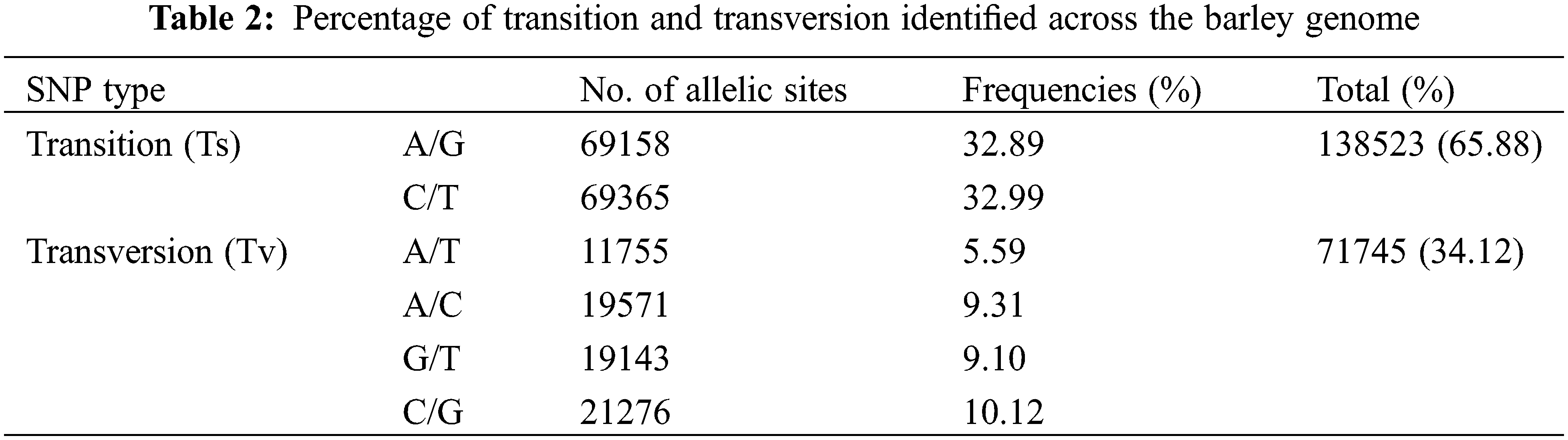
The GBS data were deposited with the National Center for Biotechnology Information (NCBI): Submission ID SUB11173831; BioProject ID PRJNA814403. A total of 210,268 SNPs were obtained for the next analysis. These SNP markers were located on all the chromosomes but were most abundant on chromosome 7 (35,892 SNPs) and least abundant on chromosome 4 (21,645 SNPs) (Fig. 1A). The SNP markers were not uniformly distributed on each chromosome, being more densely distributed at the chromosome ends. The SNP markers were classified according to their locations with-in genes or intergenic regions (Fig. 1B) and their effects on encoded proteins (Fig. 1C). It was apparent that most of the SNP markers were located in non-coding regions of the genome (intergenic type) (Fig. 1B). However, a total of 15,145 SNP markers were located in protein-coding regions, mostly representing synonymous or missense mutations, with very few of them representing nonsense mutations, which would lead to termination of translation (Fig. 1C). The nucleotide substitution patterns of the SNP markers were also compared: Transitions (Ts) (65.88%) were more frequent than transversions (Tv) (34.12%), with a ratio of 1.93. The C/T transitions and A/T transversions occurred at the highest and lowest frequencies, respectively. The frequencies of the two types of transitions were 32.99% and 32.89% for C/T and A/G, respectively. The frequencies of the four transversion types ranked as follows: C/G 10.12%, A/C 9.31%, G/T 9.10%, A/T 5.59% (Table 2).

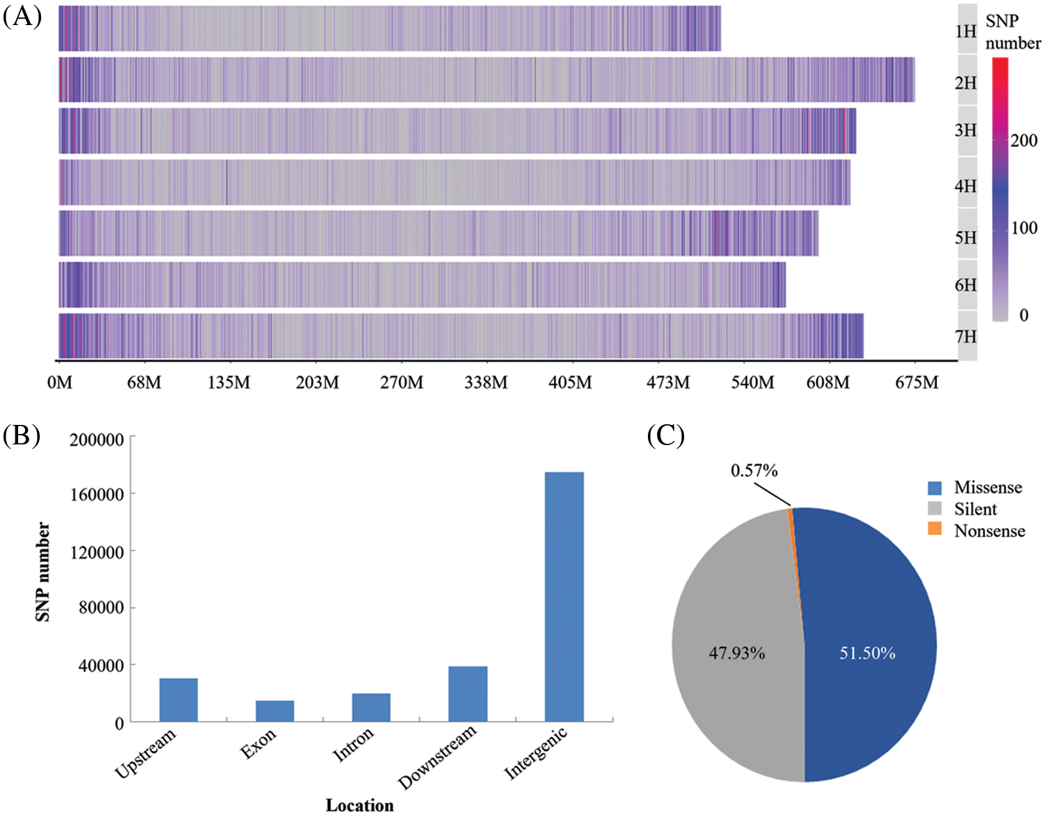
Figure 1: The distribution of identified SNPs and their classifications. (A) SNPs distribution on each barley chromosome; (B) SNPs classification according to their locations in different DNA regions; (C) SNPs classification according to their effects on protein function

3.2 Genetic Diversity Revealed by SNP Markers

All the 210,268 SNPs were of the bi-allelic type, and the effective number of alleles (Ne) was ranged from 1.0202 to 2.000 with an average of 1.3056. The major allele frequency (MAF) ranged from 0.0100 to 0.5000 with an average of 0.1350. Hardy-Weinberg equilibrium P-value (HW-P) ranged from 2.72 × 10−34 to 1.00 with an average of 0.17 (>0.05). The polymorphism information content (PIC) ranged from 0.0196 to 0.3750 with an average of 0.1642 (<0.25). The expected heterozygosity (He) ranged from 0.0198 to 0.5000 with an average of 0.1963, and the observed heterozygosity (Ho) ranged from 0 to 1.0000 with an average of 0.0696. The nucleotide diversity (π) ranged from 0.0199 to 0.5088 with an average of 0.1972.

The phylogenetic tree showed that these barley landraces clustered into three groups, named I, II and III (Fig. 2A). This classification was consistent with variation in the two morphological traits of row-type and adherence of the hulls, except for landraces B27 and B28. PCA showed that the first two principal components explained 35.55% of variance, and they were 26.08% for PC1 and 9.47% for PC2, respectively (Fig. 2B). The row-type could be separated by PC1 except for landraces B27 and B28, and the adherence of the hulls could be further separated by PC2. Although some landraces were very similar, each landrace was still well differentiated. Landraces with a similarity higher than 95% based on these SNP markers were further compared by analyzing their seed appearance (Figs. 3A and 3B). Although most of the groups had very similar seeds according to their appearance, the group of B30 and B59 was clearly different, reflecting that the seeds were different despite they were 95% similar in genetics. Meanwhile, most of the landraces with the same name (which we distinguished by numbers 1, 2, 3, etc.) were not clustered together by the analysis, and their seed appearance also differed (Figs. 3C–3E). This suggested that these barley landraces with the same name were actually different germplasm, and these mistakes might be due to recording errors or some other man-made errors.

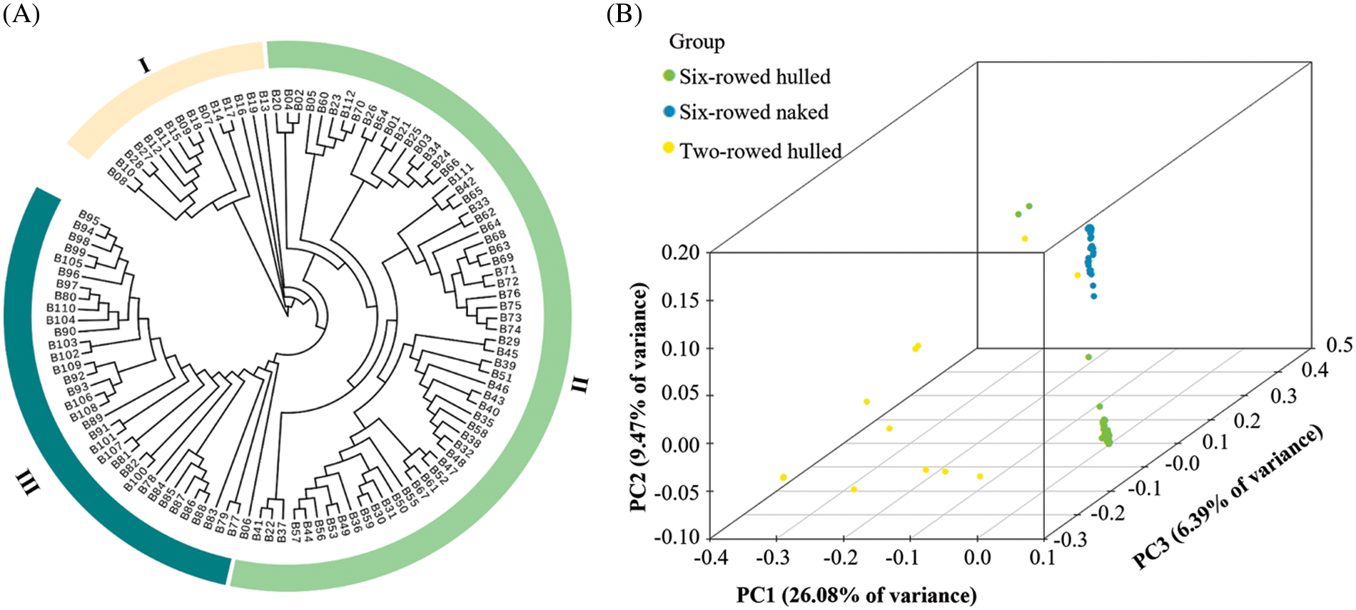
Figure 2: The phylogenetic tree and PCA of 112 barley landraces based on 210,268 SNP markers. (A) The phylogenetic tree constructed using the neighbor-joining method. (B) The 3-dimensional diagram of PCA

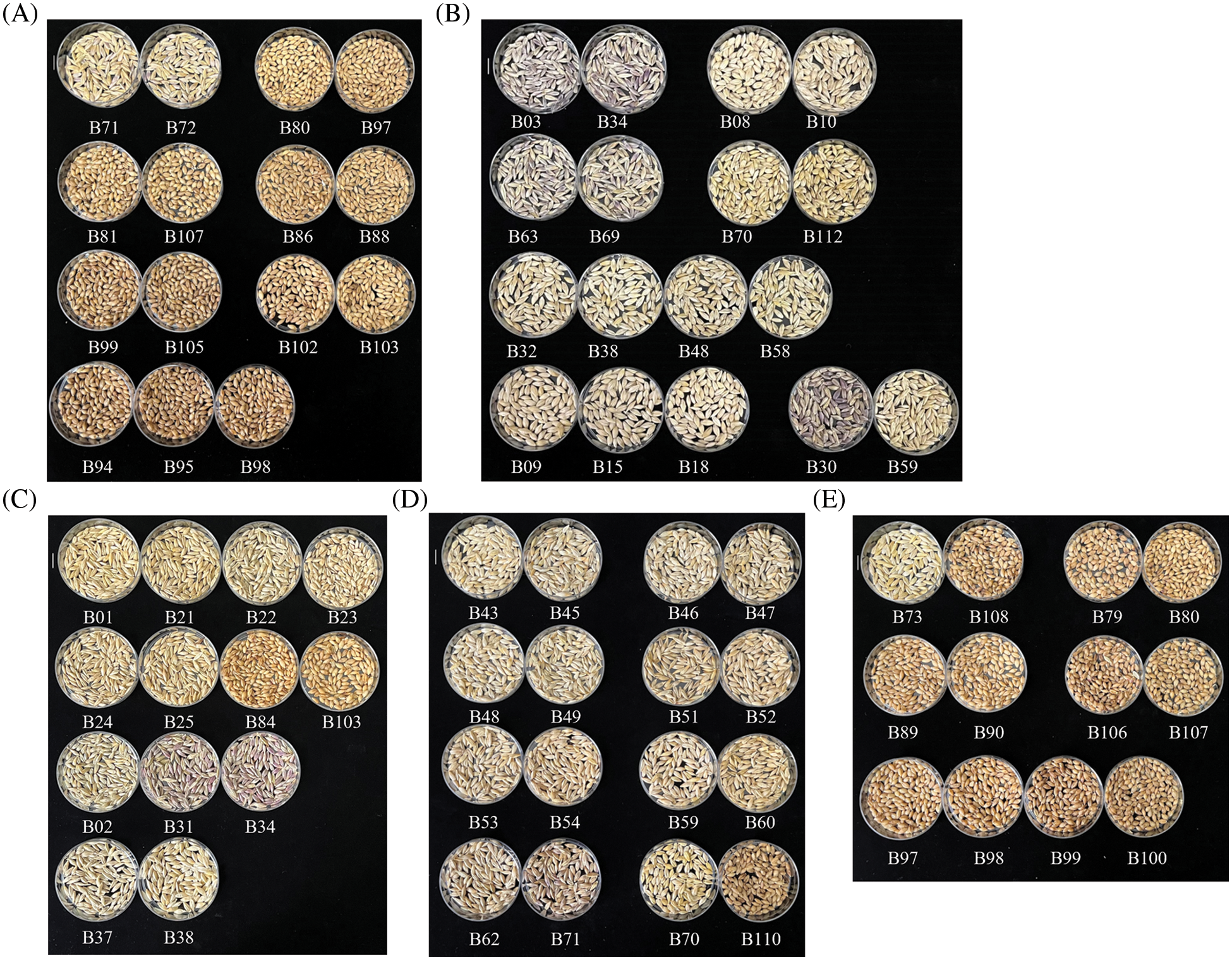
Figure 3: Seed appearances of different barley landraces. In A and B, small plates placed next to each other indicate that the seeds came from genotypes that were genetically more than 95% similar, and there were fourteen groups in total. In C–E, small plates placed next to each other indicate that the seeds came from landraces with the same name, and there were seventeen groups in total. The scale bar in each figure represents 1 cm in length

3.3 Population Structure Based on SNP Markers

A total of 29,063 SNP markers were selected for the population structure analysis. The lowest CV was detected at K = 3, indicating that K = 3 was the best for the population structure analysis (Fig. 4A). It was suggested that there were three ancestry components for the 112 barley landraces, and the morphological traits of row-type and adherence of the hulls seemed to be the major determinants of population divisions (Fig. 4B). The three sub-populations were SP1 for six-rowed and naked barley, SP2 for six-rowed and hulled barley, and SP3 for two-rowed and hulled barley. The fixation index (FST) values for the three sub-populations showed that there were greater differentiations among these three sub-populations, and the genetic relationship between SP1 and SP2 was closer than their relationship to SP3 (Fig. 4C). Some barley landraces contained two or three ancestry components, indicating that there may have been intergenic exchanges among different ancestry components.

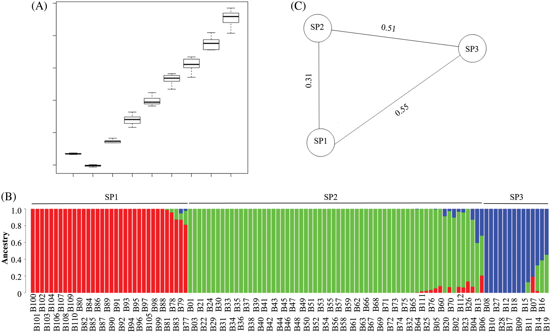
Figure 4: Population structure analysis of 112 barley landraces using 29,063 SNP markers. (A) The K value cross validation error (CV) box plot for estimation of the best K value. (B) Population structure and clustering of 112 barley landraces with K = 3. (C) The fixation index (FST) of three sub-populations based on row-type and adherence of the hulls. SP1 represents six-rowed and naked barley; SP2 represents six-rowed and hulled barley; SP3 represents two-rowed and hulled barley

Giving there is enough space, we suggest to increase font sizes for legibility.

4  Discussion

The two kinds of molecular markers of SSR and SNP are the most commonly used in barley genetic diversity analysis [4–8,15,26–34]. SSR markers were once very popular because of their good stability and easy operation. However, the frequency of SSR markers in barley populations is always relatively low, and the number of loci that can be used for genetic diversity analysis is consequently limited [4–6,8,27–29,31,34]. This makes SSRs less representative, and often means that they do not distinguish between different individuals with similar genetic backgrounds. This may lead to wrong judgments being made for the conservation of barley germplasm and the construction of core barley germplasm. SNP markers, on the other hand, can effectively solve the problem of low polymorphism. SNP-based loci detection is best based on nucleotide sequencing, but sequencing costs were once so high that it was impossible to analyze genetic diversity by nucleotide sequence analysis of every individual in a barley population. Therefore, PCR amplification-based detection of SNP loci combined with gene chip or DNA array technology was used [5,7,26,27,30,32,33,35,36]. The polymorphic markers that could be identified and used by this method were still limited. Recently, however, with the rapid development and cost reduction of nucleotide sequencing technology, it has become convenient to perform sequencing-based SNP marker genotyping for whole barley populations [15]. This will greatly accelerate the study of genetic diversity in barley.

The genetic diversity analysis for the barley landrace collection in this study identified a total of 210,268 SNPs, which would be impossible by previous methods. The SNPs were distributed almost throughout the whole genome despite they were more density toward the telomeric chromosome regions, and this was also found in other reports [7,37]. Therefore, the results based on these SNP markers will be more accurate and useful. In fact, all of the landraces could be distinguished based on these SNP markers, even those with a similarity of more than 95% (Figs. 3A–3B), and this also provided evidence that barley landraces with the same name were, in fact, different (Figs. 3C–3E). This result is different from that derived in our previous work on diversity analysis of the same barley collection based on SSR markers [8], in which many barley landraces could not be distinguished.

The clustering analyses separated these barley landraces into two groups according to the trait of row-type, while the six-row type could be further separated according to the trait of adherence of the hulls, which was not possible in the previous work. In contrast, it was found that the average PIC value of the SNP markers was lower than that of SSR markers. This has also been observed in other studies on barley [27] and might be due to the smaller number of alleles represented by the SNP markers because all the SNP markers in the study were bi-allelic. Population structure analysis was also performed in this study and the results were consistent with the cluster analysis. The study therefore not only clarified the ancestry components of the barley landrace collection, but also provided the basis for the classification of the cluster analysis.

Barley collections are generally classified according to geographic locations, growth habits or morphological characters, or combinations thereof in genetic diversity analysis [15]. Classifications based on geographic locations require that the barley germplasm used in the study originates from different regions or countries, while classifications based on growth habits often require that the barley germplasm come from different ecological areas or zones. For barley landraces originating from one region, on the other hand, classifications are likely to depend for the most part on morphological characters. In this study, the barley landrace collection from the Shanghai region could clearly be classified according to the two morphological traits of row-type and adherence of the hulls. This was also observed in our previous work [8], and that of other researchers [5,6,27,29,31,32]. Natural and artificial selection coupled with spontaneous mutations are the main methods for barley landrace breeding [1]. Therefore, we infer that genetic exchanges between barley landraces with different morphological traits must have been infrequent, leading to the separation of the landraces according to row-type and adherence of the hulls. As we know, considering the morphological traits of the wild progenitor of barley, two-row and hulled barley was the first to be domesticated, then six-row and hulled barley, and finally six-row and naked barley [38–40]. Considering traditional breeding methods, it is predictable that the genetic relationship between the latter two types of barley should be closer than that with the first type, and the fixation index (FST) values among the three types within the population were consistent with that.

Barley is a self-pollinated crop, and some are even cleistogamous, so conventional barley varieties are highly inbred and largely homozygous, while barley landraces may be less so [1,7]. The landraces in this study have undergone multiple generations of self-pollination, including single-seed propagation, so could be expected to be very close to homozygosity. However, the observed heterozygosity (Ho) showed that there were still many heterozygous loci totally in this collection (about 38.80% loci; 81,594 SNPs). There were also differences among these heterozygous loci, with 11916 loci or SNPs having an Ho value greater than 0.5, indicating that more than half of the barley landraces were heterozygous at these loci, and 63 of them even had an Ho value of 1, indicating that all the barley landraces were heterozygous at these loci except those for which data were not available. According to these heterozygous loci, the heterozygosity of barley landraces was ranged from 3.29% to 8.14% with an average of 6.90%. These results suggested that there was a relatively high level of heterozygosity in the landraces, which might also explain the problem of different landraces having the same name because of the segregation of heterozygous loci during seed propagation. Heterozygosity might also be caused by a degree of natural outcrossing in the landraces [41]. In addition, that fact that some loci were heterozygous in all the landraces suggests that these loci might not be homozygous.

5  Conclusions

In this study, we conducted genetic diversity and population structure of a barley collection by using high-throughput SNP genotyping. The genetic diversity analysis suggested that these barley landraces were totally different although some of them were very similar. Both phylogenetic tree and population structure analysis indicated that these barley landraces could be divided into three subpopulations. This was also consistent with the classification based on the two morphological traits of row-type and adherence of the hulls. Moreover, the classification might be explained by their breeding history and selection method.

Authorship: L. L. prepared barley samples, and wrote the origin draft. N. G. H. revised the manuscript. H. W. analyzed the sequencing data. Y. Z. provided barley seeds. Z. G. investigated the morphological traits. R. L. provided experiment materials. C. L. provided some suggestions for this study. Z. C. conceived and designed this study, supervised all the experiments, rewrote the manuscript. All authors have read and agreed to the published version of the manuscript.

Data Availability Statement: The GBS data of the 112 barley landraces were available at https://www.ncbi.nlm.nih.gov/bioproject/814403.

Funding Statement: This research was funded by the Shanghai Agriculture Applied Technology Development Program (Grant No. 2019-02-08-00-08-F01109), the Climbing Plan (Grant No. PG22211) and the Ear-Marked Fund for CARS (Grant No. CARS-05-01A-02). N. G. H. is supported at Rothamsted Research by the Biotechnology and Biological Sciences Research Council (BBSRC) via the Designing Future Wheat Programme (BB/P016855/1).

Conflicts of Interest: The authors declare that they have no conflicts of interest to report regarding the present study.

Appendix:

Table S1: Quality control of the DNA-seq data

References

1. Kumar, A., Verma, R. P. S., Singh, A., Kumar Sharma, H., Devi, G. (2020). Barley landraces: Ecological heritage for edaphic stress adaptations and sustainable production. Environmental and Sustainability Indicators, 6(1), 100035. DOI 10.1016/j.indic.2020.100035. [Google Scholar] [CrossRef]
2. Lü, B., Wu, J. J., Fu, D. L. (2017). Constructing the barley model for genetic transformation in Triticeae. Journal of Integrative Agriculture, 14(3), 453–468. DOI 10.1016/S2095-3119(14)60935-7. [Google Scholar] [CrossRef]
3. Mascher, M., Gundlach, H., Himmelbach, A., Beier, S., Twardziok, S. O. et al. (2017). A chromosome conformation capture ordered sequence of the barley genome. Nature, 544(7651), 427–433. DOI 10.1038/nature22043. [Google Scholar] [CrossRef]
4. Ferreira, J. R., Pereira, J. F., Turchetto, C., Minella, E., Consoli, L. et al. (2016). Assessment of genetic diversity in Brazilian barley using SSR markers. Genetics and Molecular Biology, 39(1), 86–96. DOI 10.1590/1678-4685-gmb-2015-0148. [Google Scholar] [CrossRef]
5. Elakhdar, A., Kumamaru, T., Kevin, K. P., Brueggeman, R., Capo-chichi, L. et al. (2018). Assessment of genetic diversity in Egyptian barley (Hordeum vulgare L.) genotypes using SSR and SNP marker. Genetic Resource and Crop Evolution, 65(7), 1937–1951. DOI 10.1007/s10722-018-0666-x. [Google Scholar] [CrossRef]
6. Mohammadi, S. A., Abdollahi Sisi, N., Sadeghzadeh, B. (2020). The influence of breeding history, origin and growth type on population structure of barley as revealed by SSR markers. Scientific Report, 10(1), 19165. DOI 10.1038/s41598-020-75339-4. [Google Scholar] [CrossRef]
7. Dziurdziak, J., Gryziak, G., Groszyk, J., Podyma, W., Boczkowska, M. (2021). DArTseq genotypic and phenotypic diversity of barley landraces originating from different countries. Agronomy, 11(11), 2330. DOI 10.3390/agronomy11112330. [Google Scholar] [CrossRef]
8. Chen, Z. W., Lu, R. J., Zou, L., Du, Z. Z., Gao, R. H. (2012). Genetic diversity analysis of barley landraces and cultivars in the Shanghai region of China. Genetic and Molecular Research, 11(1), 644–650. DOI 10.4238/2012.March.16.2. [Google Scholar] [CrossRef]
9. Elshire, R. J., Glaubitz, J. C., Sun, Q., Poland, J. A., Kawamoto, K. et al. (2011). A robust, simple genotyping-by-sequencing (GBS) approach for high diversity species. PLoS One, 6(5), e19379. DOI 10.1371/journal.pone.0019379. [Google Scholar] [CrossRef]
10. Wendler, N., Mascher, M., Nöh, C., Himmelbach, A., Scholz, U. et al. (2014). Unlocking the secondary gene-pool of barley with next-generation sequencing. Plant Biotechnology Journal, 12(8), 1122–1131. DOI 10.1111/pbi.12219. [Google Scholar] [CrossRef]
11. Qi, P., Gimode, D., Saha, D., Schröder, S., Chakraborty, D. et al. (2018). UGbS-flex, a novel bioinformatics pipeline for imputation-free SNP discovery in polyploids without a reference genome: Finger millet as a case study. BMC Plant Biology, 18(1), 117. DOI 10.1186/s12870-018-1316-3. [Google Scholar] [CrossRef]
12. Tang, W., Wu, T., Ye, J., Sun, J., Jiang, Y. et al. (2016). SNP-based analysis of genetic diversity reveals important alleles associated with seed size in rice. BMC Plant Biology, 16(1), 93. DOI 10.1186/s12870-016-0779-3. [Google Scholar] [CrossRef]
13. Eltaher, S., Sallam, A., Belamkar, V., Emara, H. A., Nower, A. A. et al. (2018). Genetic diversity and population structure of F(3:6) Nebraska winter wheat genotypes using genotyping-by-sequencing. Frontiers in Genetics, 9, 76. DOI 10.3389/fgene.2018.00076. [Google Scholar] [CrossRef]
14. Wang, N., Yuan, Y., Wang, H., Yu, D., Liu, Y. et al. (2020). Applications of genotyping-by-sequencing (GBS) in maize genetics and breeding. Scientific Reports, 10(1), 16308. DOI 10.1038/s41598-020-73321-8. [Google Scholar] [CrossRef]
15. Milner, S. G., Jost, M., Taketa, S., Mazón, E. R., Himmelbach, A. et al. (2019). Genebank genomics highlights the diversity of a global barley collection. Nature Genetics, 51(2), 319–326. DOI 10.1038/s41588-018-0266-x. [Google Scholar] [CrossRef]
16. McKenna, A., Hanna, M., Banks, E., Sivachenko, A., Cibulskis, K. et al. (2010). The genome analysis toolkit: A map reduce framework for analyzing next-generation DNA sequencing data. Genome Research, 20(9), 1297–1303. DOI 10.1101/gr.107524.110. [Google Scholar] [CrossRef]
17. Danecek, P., Auton, A., Abecasis, G., Albers, C. A., Banks, E. et al. (2011). The variant call format and VCFtools. Bioinformatics, 27(15), 2156–2158. DOI 10.1093/bioinformatics/btr330. [Google Scholar] [CrossRef]
18. Cingolani, P., Platts, A., Wang le, L., Coon, M., Nguyen, T. et al. (2012). A program for annotating and predicting the effects of single nucleotide polymorphisms, SnpEff. Fly, 6(2), 80–92. DOI 10.4161/fly.19695. [Google Scholar] [CrossRef]
19. Nei, M., Roychoudhury, A. K. (1974). Genic variation within and between the three major races of man, Caucasoids, Negroids, and Mongoloids. American Journal of Human Genetics, 26(4), 421–443. [Google Scholar]
20. Botstein, D., White, R. L., Skolnick, M., Davis, R. W. (1980). Construction of a genetic linkage map in man using restriction fragment length polymorphisms. American Journal of Human Genetics, 32(3), 314–331. [Google Scholar]
21. Ruan, J., Li, H., Chen, Z., Coghlan, A., Coin, L. J. et al. (2008). TreeFam: 2008 update. Nucleic Acids Research, 36, D735–D740. DOI 10.1093/nar/gkm1005. [Google Scholar] [CrossRef]
22. Yang, J., Lee, S. H., Goddard, M. E., Visscher, P. M. (2011). GCTA: A tool for genome-wide complex trait analysis. American Journal of Human Genetics, 88(1), 76–82. DOI 10.1016/j.ajhg.2010.11.011. [Google Scholar] [CrossRef]
23. Alexander, D. H., Novembre, J., Lange, K. (2009). Fast model-based estimation of ancestry in unrelated individuals. Genome Research, 19(9), 1655–1664. DOI 10.1101/gr.094052.109. [Google Scholar] [CrossRef]
24. Rousset, F. (2008). genepop’007: A complete re-implementation of the genepop software for Windows and Linux. Molecular Ecology Resources, 8(1), 103–106. DOI 10.1111/j.1471-8286.2007.01931.x. [Google Scholar] [CrossRef]
25. Wright, S. (1978). Evolution and the genetics of populations, volume 4: Variability within and among natural population. Chicago, USA: University of Chicago Press. [Google Scholar]
26. Al-Abdallat, A. M., Karadsheh, A., Hadadd, N. I., Akash, M. W., Ceccarelli, S. et al. (2017). Assessment of genetic diversity and yield performance in Jordanian barley (Hordeum vulgare L.) landraces grown under Rainfed conditions. BMC Plant Biology, 17(1), 191. DOI 10.1186/s12870-017-1140-1. [Google Scholar] [CrossRef]
27. Bengtsson, T., Manninen, O., Jahoor, A., Orabi, J. (2017). Genetic diversity, population structure and linkage disequilibrium in Nordic spring barley (Hordeum vulgare L. subsp. vulgare). Genetic Resource and Crop Evolution, 64(8), 2021–2033. DOI 10.1007/s10722-017-0493-5. [Google Scholar] [CrossRef]
28. Gong, X., Westcott, S., Li, C., Yan, G., Lance, R. et al. (2009). Comparative analysis of genetic diversity between Qinghai-Tibetan wild and Chinese landrace barley. Genome, 52(10), 849–861. DOI 10.1139/g09-058. [Google Scholar] [CrossRef]
29. Kumar, P., Banjarey, P., Malik, R., Tikle, A. N., Verma, R. P. S. (2020). Population structure and diversity assessment of barley (Hordeum vulgare L.) introduction from ICARDA. Journal of Genetics, 99, 70. [Google Scholar]
30. Lister, D. L., Jones, H., Jones, M. K., O’Sullivan, D. M., Cockram, J. (2013). Analysis of DNA polymorphism in ancient barley herbarium material: Validation of the KASP SNP genotyping platform. Taxon, 62(4), 779–789. DOI 10.12705/624.9. [Google Scholar] [CrossRef]
31. Malysheva-Otto, L. V., Ganal, M. W., Röder, M. S. (2006). Analysis of molecular diversity, population structure and linkage disequilibrium in a worldwide survey of cultivated barley germplasm (Hordeum vulgare L.). BMC Genetics, 7(1), 6. DOI 10.1186/1471-2156-7-6. [Google Scholar] [CrossRef]
32. Muñoz-Amatriaín, M., Cuesta-Marcos, A., Endelman, J. B., Comadran, J., Bonman, J. M. et al. (2014). The USDA barley core collection: Genetic diversity, population structure, and potential for genome-wide association studies. PLoS One, 9(4), e94688. DOI 10.1371/journal.pone.0094688. [Google Scholar] [CrossRef]
33. Wenzl, P., Carling, J., Kudrna, D., Jaccoud, D., Huttner, E. et al. (2004). Diversity arrays technology (DArT) for whole-genome profiling of barley. PNAS, 101(26), 9915–9920. DOI 10.1073/pnas.0401076101. [Google Scholar] [CrossRef]
34. Yahiaoui, S., Igartua, E., Moralejo, M., Ramsay, L., Molina-Cano, J. L. et al. (2008). Patterns of genetic and eco-geographical diversity in Spanish barleys. Theoretische und angewandte Genetik, 116(2), 271–282. DOI 10.1007/s00122-007-0665-3. [Google Scholar] [CrossRef]
35. Bayer, M. M., Rapazote-Flores, P., Ganal, M., Hedley, P. E., Macaulay, M. et al. (2017). Development and evaluation of a barley 50k iSelect SNP array. Frontiers in Plant Science, 8, 1792. DOI 10.3389/fpls.2017.01792. [Google Scholar] [CrossRef]
36. Torkamaneh, D., Laroche, J., Bastien, M., Abed, A., Belzile, F. (2017). Fast-GBS: A new pipeline for the efficient and highly accurate calling of SNPs from genotyping-by-sequencing data. BMC Bioinformatics, 18(1), 5. DOI 10.1186/s12859-016-1431-9. [Google Scholar] [CrossRef]
37. Kang, L., Qian, L., Zheng, M., Chen, L., Chen, H. et al. (2017). Genomic insights into the origin, domestication and diversification of Brassica juncea. Nature Genetics, 53(9), 1392–1402. DOI 10.1038/s41588-021-00922-y. [Google Scholar] [CrossRef]
38. Komatsuda, T., Pourkheirandish, M., He, C., Azhaguvel, P., Kanamori, H. et al. (2007). Six-rowed barley originated from a mutation in a homeodomain-leucine zipper I-class homeobox gene. PNAS, 104(4), 1424–1429. [Google Scholar]
39. Ramsay, L., Comadran, J., Druka, A., Marshall, D. F., Thomas, W. T. et al. (2011). INTERMEDIUM-C, a modifier of lateral spikelet fertility in barley, is an ortholog of the maize domestication gene TEOSINTE BRANCHED 1. Nature Genetics, 43(2), 169–172. DOI 10.1038/ng.745. [Google Scholar] [CrossRef]
40. Taketa, S., Amano, S., Tsujino, Y., Sato, T., Saisho, D. et al. (2008). Barley grain with adhering hulls is controlled by an ERF family transcription factor gene regulating a lipid biosynthesis pathway. PNAS, 105(10), 4062–4067. DOI 10.1073/pnas.0711034105. [Google Scholar] [CrossRef]
41. Parzies, H., Spoor, W., Ennos, R. (2008). Outcrossing rates of barley landraces from Syria. Plant Breeding, 119(6), 520–522. DOI 10.1046/j.1439-0523.2000.00532.x. [Google Scholar] [CrossRef]