Improved Leaf Chlorophyll Content Estimation with Deep Learning and Feature Optimization Using Hyperspectral Measurements

1  Introduction

Chlorophyll is an important pigment in green plants. Its content variations possess an important effect on botanic growth status and photosynthetic capacity and are directly related to stress conditions and the senescence process [1]. Accurate estimation of its content and fluctuation is crucial and thus could provide the basis for plant growth condition analysis [2]. Since chlorophyll exhibits obvious absorption features within blue and red bands, it is possible to employ remote sensing and spectroscopic techniques for non-destructively determination of its content, and plentiful researchers thus have developed various retrieval methods, including empirical methods using the spectral index, non-parametric statistic methods, inversion of radiation transfer model (RTM) and hybrid methods, for chlorophyll content assessment [2–4].

Compared with these methods, the convolutional neural network (CNN) excels in excellent representation learning ability and biological similarity, which makes it suitable for hyperspectral data processing [5–7]. Abundant research has been carried out to apply CNN for agronomic parameter retrieval. For instance, Barman et al. [8] utilized a CNN model with 12 color features from tea leaf images to assess chlorophyll content. The model achieved good accuracies with a mean absolute error (MAE) of 3.01 μg/cm2 and a root mean square error (RMSE) of 4.18 μg/cm2. Shi et al. [9] combined reflectance ranging from 400 to 2450 nm as input features with AlexNet for estimation of leaf carotenoids and chlorophyll content. Their results showed that AlexNet behaved with better accuracies (a coefficient of determination (R2) of 0.91, and a RMSE of 6.36 μg/cm2) for leaf chlorophyll content retrieval when compared with that from traditional machine learning techniques. Zhou et al. [10] used seven image features representing plant height, canopy color, and canopy texture to build a hybrid CNN model for soybean yield estimation, which showed accurate results for yield prediction (R2 = 0.78; RMSE = 391 kg/ha), Prilianti et al. [11] analyzed chlorophylls, carotenoids, and anthocyanins in plant leaves using multispectral digital images, and input the 10-channel multispectral images into a CNN for comprehensive prediction of pigmentation, and the results showed that the CNN was able to identify the relationship between the digital images of the leaves and the pigmentation content very well, and the optimal mean squared error reached 0.0037. Considering that full-range hyperspectral data may contain redundant information, several researchers adopted methods for data dimensionality reduction when dealing with hyperspectral reflectance data for parameter retrieval. Elsherbiny et al. [12] employed the principal component analysis (PCA) method for hyperspectral dimensionality reduction, and extracted features were then used for back propagation neural network (BPNN) in estimating paddy rice canopy water content, and it was found that the use of PCA algorithm improved model accuracy. Zhang et al. [13] combined successive projection algorithm (SPA) and competitive adaptive reweighting algorithm (CARS) with machine learning algorithms to effectively eliminate hyperspectral redundancy, decrease input dimensionality, and thus enhance model operation efficiency. In addition to data dimensionality reduction of input features for CNN modeling, some researchers focused on various approaches, such as transfer learning (TL), to perfect model framework or hyper-parameters so as to improve network convergence rate, alleviate overfitting, and thus increase model generalization abilities [14]. Based on transfer learning and residual networks, Wang et al. [15] proposed a TL-SE-ResNeXt-101 model for crop disease identification, which improved the convergence speed of the model and significantly improved the accuracy of crops diseases identification in real circumstances compared to models without transfer learning. Malathi et al. [16] applied transfer learning to a pest dataset by fine-tuning hyper-parameters of the ResNet-50 model and the accuracy of the fine-tuned model was 95.01%.

The above-mentioned literature has indeed enriched CNN methodologies in agronomic applications. In the research process of chlorophyll content retrieval, insufficient data samples could be frequently encountered when dealing with CNN models [17]. Although some researchers tried to use radiation transfer models (RTMs) for simulation to expand data size for model establishment, combinations of different parameters might produce simulations that were obviously different from corresponding measured data, moreover, differences between simulated and corresponding measured data could not be quantified under most circumstances. Thus, these simulated data when used for CNN modeling might incur unexplainable results. Compared with hyperspectral reflectance data, spectral indices (SIs) that were calculated from several specific wavebands’ reflectance, were commonly constructed and utilized to extract plant characteristics and could be considered to reduce hyperspectral dimensionality with high collinearity. Despite a large amount of SIs having been proposed for different purposes, studies on SIs selection and use for the optimization of CNN model establishment when dealing with crop chlorophyll content retrieval were still limited [18]. In addition, most research concerning CNN models for parameter inversion focused on estimation accuracies as the main index, which in turn might incur overfitting problems to some extent. Thus, it is imperative to optimize model structure so as to ensure high model accuracies while improving model convergence rate and avoiding parameter overfitting problems. Thus, in the present study, we aimed to analyze the effects of combining synthetic data for modeling, input feature optimization model convergence issues, and generalization for accurate and robust estimation of plant LCC with a deep learning framework (i.e., ResNet-18). The specific objectives were to: i) evaluate the accuracies of abundant leaf reflectance simulation based on measured foliar hyperspectral using a GPR model; ii) analyze the influence of adding simulated data on the assessment of leaf chlorophyll content retrieval with ResNet-18 using raw reflectance data (400–1000 nm); iii) investigate the effect of input feature selection on the performance of leaf chlorophyll content estimation, based on various spectral indices; iv) assess the generalization capability when combined transfer learning with ResNet-18 for improved LCC modeling.

2  Materials and Methods

2.1 Measured and Synthetic Data

(1) ANGERS dataset

In order to investigate the mentioned aspects using deep learning frameworks for leaf chlorophyll content assessment, public data, i.e., ANGERS dataset (http://opticleaf.ipgp.fr/) (accessed on 23 January 2025), which included both leaf biochemical parameters and leaf spectral data for temperate plants (39 plant species, including deciduous trees/shrubs) collected by the French National Institute of Agricultural Research (INRA) in 2003, was used. The leaf spectrum containing directional hemispherical reflection and transmission was measured using an ASD FieldSpec spectrometer combined with an integrating sphere. The spectral data was characterized with a spectral resolution of 1 nm ranging from 400 to 2400 nm. Leaf biochemical compositions, such as chlorophyll a and b, carotenoids, equivalent water thickness (EWT), and leaf mass per area (LMA), were determined using standard laboratory methods. Among which, pigment contents were measured with spectrophotometric techniques, i.e., selected leaves were first dissolved in 95% ethanol, and leaf chlorophyll a chlorophyll b, and carotenoid contents were calculated with solutions’ absorption features at wavelengths of 470, 648.6, and 664.2 nm, respectively. Detailed descriptions of the ANGERS dataset can be found in the literature [19]. Since the absorption features are mainly within the visible wavelength range, leaf reflectance ranging from 400 to 1000 nm was considered, and a total of 276 samples were used for leaf chlorophyll content estimation.

(2) Simulated Data

To assess the influence of data size on leaf chlorophyll content retrieval using a deep learning model, different sizes of simulations were generated with the measured ANGERS dataset and Gaussian process regression (GPR) methods. The simulation process primarily involved three steps: (1) Model data, including 276 leaf-measured spectra and corresponding leaf chlorophyll content. Here, leaf chlorophyll content was used as input features to simulate spectra data as model output. The total amount of ANGERS data (n = 276) was randomly divided into 60% for model calibration and remnant 40% for model validation. (2) Model training and validation. GPR was chosen as a multi-output machine learning algorithm, combined with a calibration dataset to obtain a 400–1000 nm reflectance model, and model accuracy was evaluated with independent validation data. (3) Data simulation. Combining with leaf chlorophyll content numerical characteristics (i.e., maximum, minimum, mean, and standard deviation) and its normal distribution, as well as the number of simulations, 400–1000 nm leaf reflectance data were modeled based on the established multi-output model, so as to obtain a different number of datasets (n = 200, 500, 800, and 1000). Simulations were performed using the Automated Radiative Transfer Models Operator (ARTMO) Toolbox version 3.29 within Matlab software. The ARTMO is a software package that provides tools for running and inverting a suite of plant RT models, and it facilitates consistent and intuitive user interaction, thereby streamlining model setup, running, storing, and output plotting for data further analysis [20].

2.2 Spectral Index Features

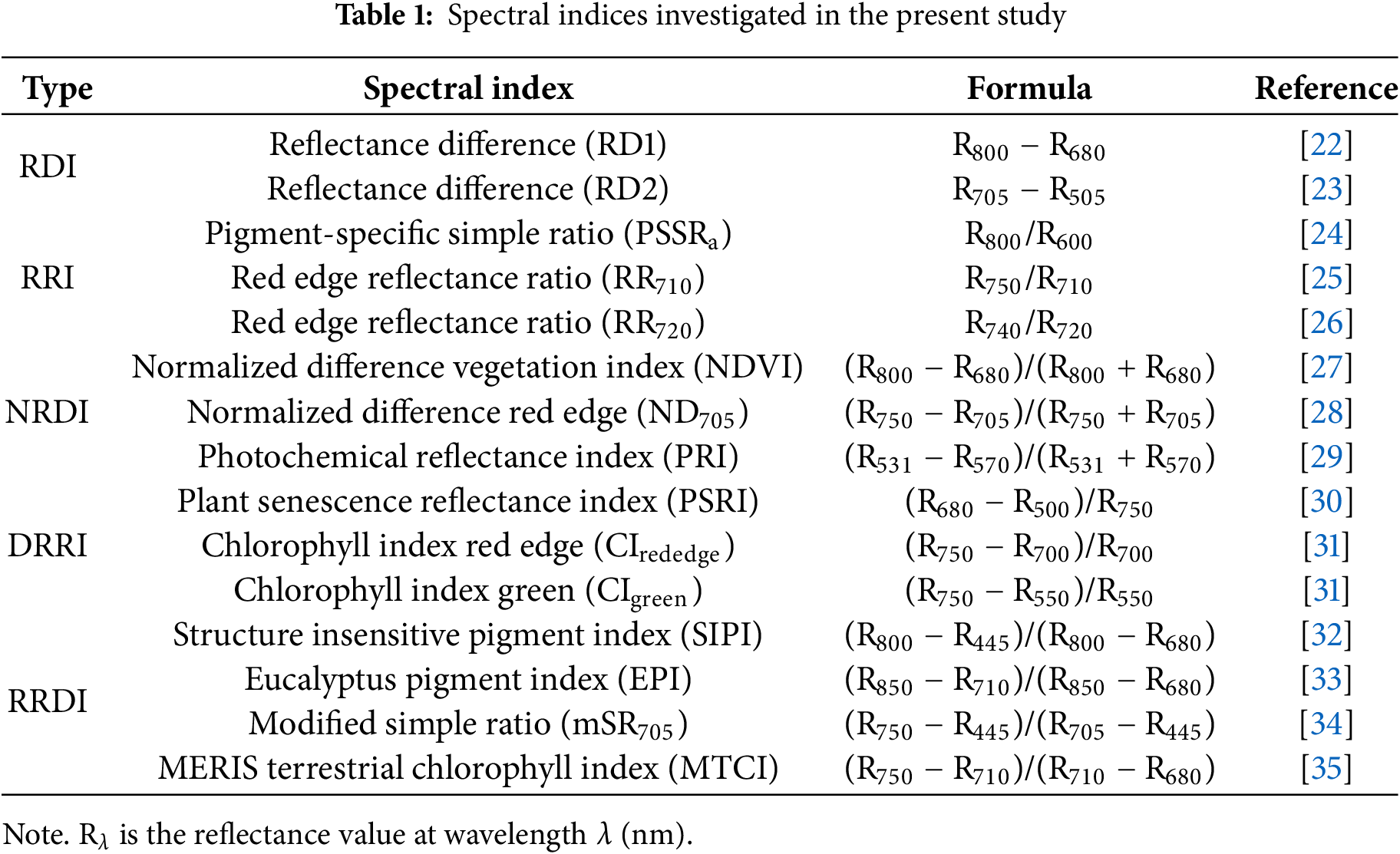
Apart from reflectance data (400–1000 nm) used as model input, spectral indices were also investigated as input features for model building. Here different types of spectral indices were summarized and classified into five categories [21]: 1) Reflectance difference index (RDI). Which was expressed as the reflectance of one band subtracted from that of another one; 2) Reflectance ratio index (RRI) that uses one band reflected spectra divided by that of another one; 3) Normalized reflectance difference index (NRDI), which utilized the difference value of reflectance from two individual wavebands divided by their addition value; 4) Difference of reflectance ratio index (DRRI). This form was a combination of RDI and RRI, where the numerator was the difference value of reflectance from two individual wavebands, while, the denominator was just the reflectance value of one waveband; 5) Ratio of reflectance difference index (RRDI). Different from DRRI formation, the numerator and denominator of RRDI both comprised different values of reflectance from two individual wavebands, and one waveband was repeatedly used in both the numerator and denominator. Detailed information about these spectral indices is listed in Table 1.

2.3 Competitive Adaptive Reweighted Sampling (CARS)

Even though varied spectral indices were selected as CNN model input, redundant information might still occur when model training. A feature selection algorithm, i.e., competitive adaptive reweighted sampling (CARS) was thus used. The method could choose features based on their significant regression coefficients in the partial least squares (PLS) model, utilizing the adaptive reweighted sampling (ARS) technique. Low-weight input features and optimal variables combination through cross-validation process could be determined with the lowest root mean square error of the cross-validation (RMSECV). The algorithm comprised the following key steps:

1) The PLS model was constructed using a Monte Carlo sampling approach, where 80% of calibration samples were randomly chosen for modeling in each iteration, while the remaining 20% were reserved for prediction. Sampling number N for Monte Carlo should be predetermined, and PLS model weights need to be recorded for each sampling process.

2) Exponential decay function (EDF) was utilized to eliminate features with minimal regression weights. When the PLS model was established based on Monte Carlo sampling, the ratio R of variables number determined by the I sampling was determined by the following formulas:

R=μe−ki (1)

μ=(n2)1N−1 (2)

k=lnn2N−1 (3)

where n was the total number of features that were used for PLS modeling.

3) During each sampling, PLS modeling was executed by selecting R*n variables from the number of variables in the previous sampling, employing the adaptive reweighted sampling (ARS) method to compute RMSECV.

4) After N times of sampling, the CARS algorithm could obtain a feature set of N group candidates, and corresponding RMSECV values, the optimal feature subset was determined with the minimum RMSECV values.

2.4 ResNet-18 Framework

ResNet-18 was used as a backbone network in the present study, its main components consist of an input layer, a convolutional layer, four residual modules, a fully connected network, and an output layer. Here, the input layer was composed of either reflectance data from 400–1000 nm wavebands, or specific calculated spectral indices; while LCC was estimated as output. In order to better adapt spectra reflectance data or spectral indices features to ResNet-18, the network structure was changed: Firstly, all two-dimensional convolutional layers were adjusted to one-dimensional convolutional layers; secondly, the original down-sampling convolution layer of the first input was modified from the 7 × 1 to 3 × 1, so as to make better use of spectral reflectance or spectral indices. The ANGERS dataset was randomly divided into two parts (training and validation), each with a number of 138. Simulated data with different amounts of 200, 500, 800, and 1000 were added to the training portion, respectively, in order to investigate the effect of varied data sizes on the performance of the ResNet-18. Before entering the network, input data were standardized using mean values and standard deviation of each channel (reflectance from 400–1000 nm wavebands) or feature (various spectral indices). The best settings for the ResNet-18 model were as follows: the path parameter was set to 128, and the network was trained in 1000 iterations. The learning rate was fixed to 0.01, while, the Adam optimization algorithm was adopted. Mean Squared Error (MSE) loss function and batch normalization were further utilized to mitigate the overfit problem during network training. In addition, a transfer learning method was added to the ResNet-18 framework (i.e., TL-ResNet-18) to investigate network convergence rate and model generalization capability. Training of TL-ResNet-18 was divided into two parts: firstly, all simulated data were used to train the network so as to gain model coarse parameters; the second part was to fine-tune model parameters which were obtained in the first part, using the ANGERS dataset with the same data partition when ResNet-18 alone was trained and validated. In terms of TL-ResNet-18 modeling, input data were specific spectral indices that were selected with the CARS algorithm. The detailed flowchart is presented in Fig. 1.

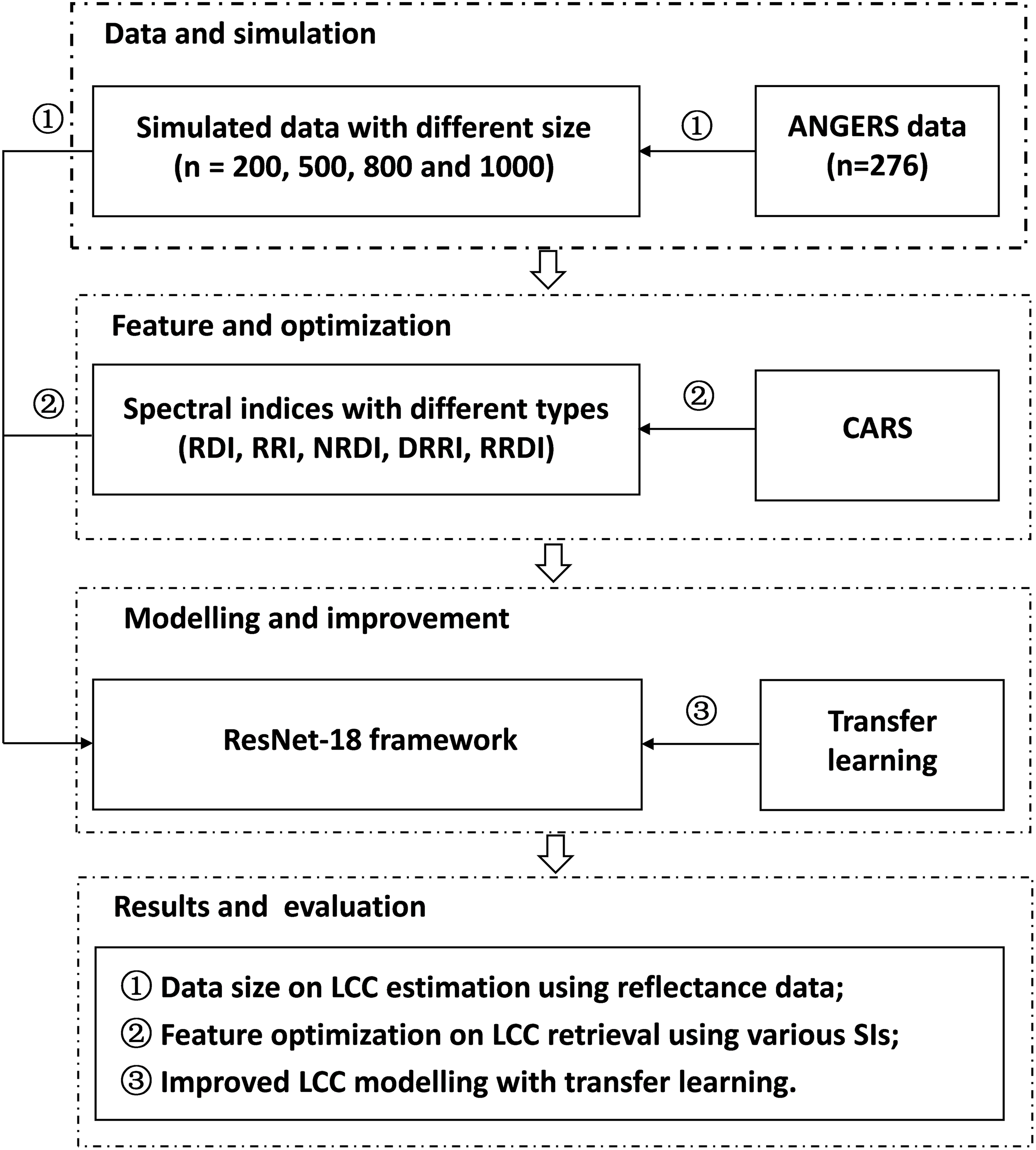
Figure 1: Flowchart of LCC estimation with ResNet-18 deep learning framework

2.5 Model Accuracy Evaluation

For the multi-output model with GPR methods, root mean square error (RMSE), mean absolute error (MAE), relative root mean square error (RRMSE), and normalized root mean square error (NRMSE) were chosen to compare simulated reflectance from 400 to 1000 nm with leaf measured spectra within this wave range. While, for LCC retrieval with ResNet-18 or TL-ResNet-18 approaches, coefficient of determination (R2), RMSE, and relative percent deviation (RPD) were selected. In addition, accuracy (A) and precision (P) mentioned in [36] were also considered as indexes for validation results.

3  Result

3.1 Comparison between Emulated and Measured Hyperspectral Data

The overall evaluation accuracies of GPR training and validation models for 400–1000 nm reflectance simulation are presented in Table 2. Results showed that the GPR model training process behaved with a similar performance to that of the validation procedure, which indicates the robustness of multi-output GPR for modeling. Detailed comparison between simulation and measured data curves for 400–1000 nm reflectance was further investigated (Fig. 2). Results in Fig. 2a showed the difference between best (or worst) simulated curves and correspondingly measured reflectance data. It could be seen that the best simulation curve was close to that of correspondingly measured data, apart from that reflectance from 400–500 nm and 600–700 nm exhibited slight differences. In contrast, the worst simulation exhibited a poor similarity to the correspondingly measured curve: obvious difference occurred in the region from 400 to 780 nm, where reflectance at 680 nm performed with the largest dissimilarity (reflectance difference value of about 0.2). Apart from best and worst simulations, the statistical overview for synthetic and measured reflectance in Fig. 2b showed that curves of average values from simulated and measured reflected data exhibited the same values within the 400–1000 nm wave range. In terms of standard deviation curves, reflectance standard deviation boundaries of emulated reflectance were less varied than that of ANGERS data. Moreover, standard deviation values were slighter larger in 500–700 nm region for both measured and simulated data, compared with reflectance from other wavebands. In addition, maximum and minimum reflectance for simulated data showed limited variations compared with that of measured data, while measured ANGERS data behaved with a much larger upper bound in the visible range (400–780 nm).

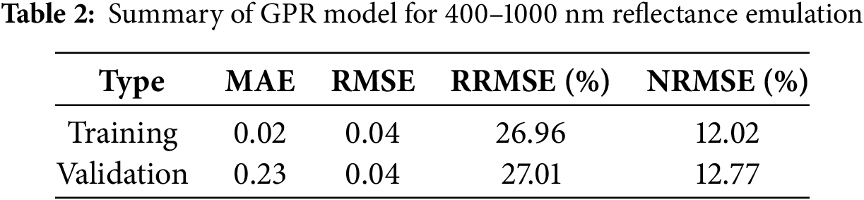
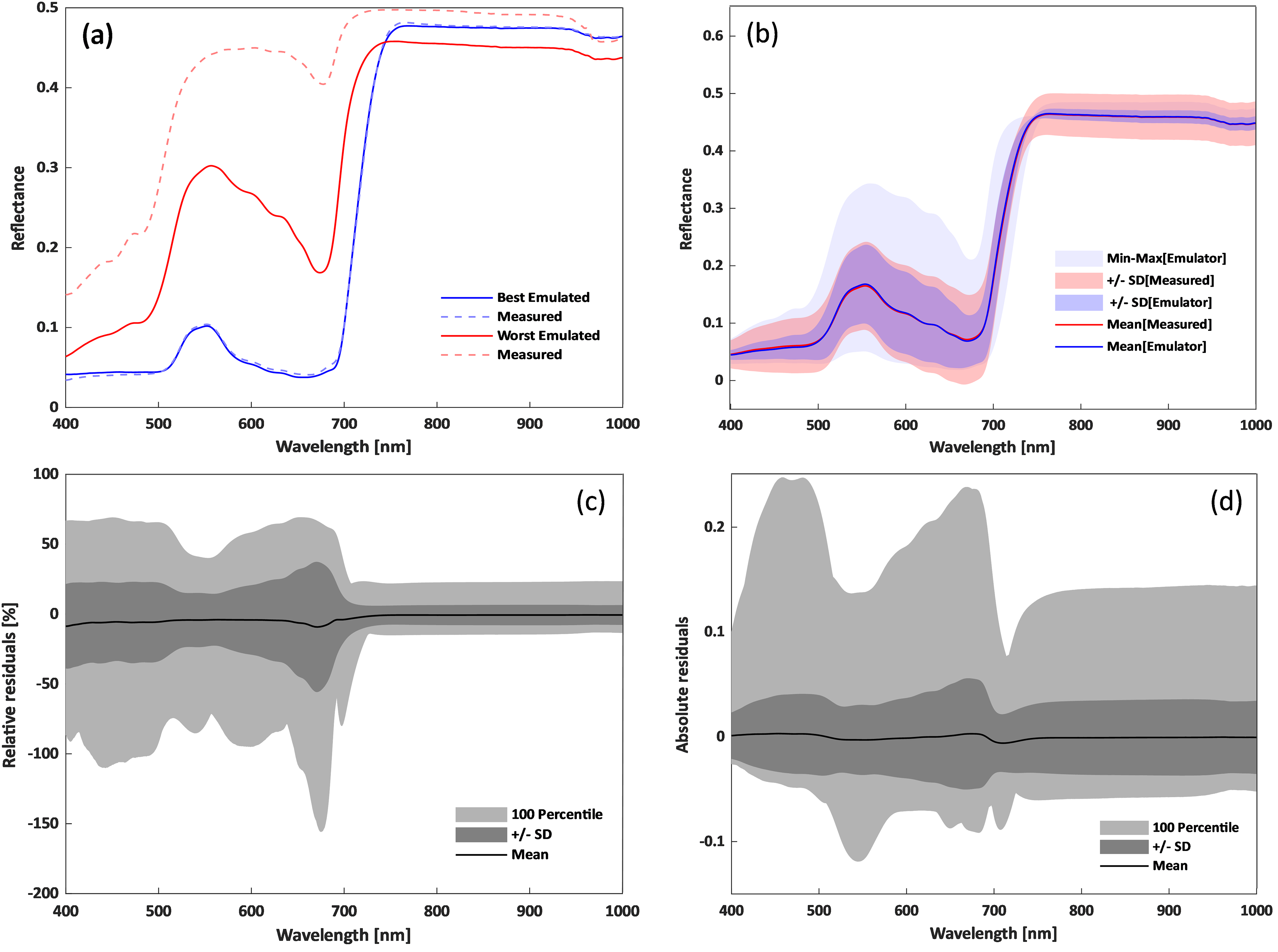
Figure 2: Comparison of emulated and ANGERS-measured spectral data ranging from 400 to 1000 nm. (a) was best and worst simulation vs. measured data, (b)–(d) were statistical overview, relative residuals, and absolute residuals between synthetic and measured reflectance, respectively. SD referred to standard deviation

Relative residual values between simulated and measured data ranging from 400 to 1000 nm are presented in Fig. 2c. Results showed that variations of relative residual mean values (black line in Fig. 2c) were basically around 0 in 400–1000 nm wavebands, with a slight fluctuation around 680 nm. Similar to the variations results of reflectance SD values in Fig. 2b, relative residual SD values also exhibited a larger variation (varied from −30% to 20%) in 400–750 nm wave region compared to those values (−7%–6%) after 750 nm. Absolute maximum relative residual SD occurred around 680 nm with a value of 55.74%. Similarly, upper and lower boundaries of relative residual values behaved with obvious large fluctuation from 400 to 750 nm waveband range, with 680 nm exhibiting the maximum relatively residual value (155.56%). In terms of absolute residual statistics in Fig. 2d, its mean values were close to 0 within 400–1000 nm as well. In comparison, maximum and minimum SD values of absolute residual exhibited a moderate oscillation, with values slightly larger from 400 to 700 nm than values in 700–1000 nm. As for its upper and lower bounds, maximum and minimum values behaved with noteworthy variations in 400–700 nm, with 480 and 680 nm exhibiting absolute residual values larger than 0.2.

3.2 Effect of Synthetic Data Size on LCC Retrieval with ResNet-18

To investigate the effect of varied data size on the performance of ResNet-18 for LCC estimation, different amounts of simulated data (i.e., 200, 500, 800, and 1000) were combined with the training part of ANGERS data (n = 138) for ResNet-18 modeling using reflectance from 400 to 1000 nm, respectively. Remanent ANGERS data (n = 138) were then used for model validation, and validation results are presented in Fig. 3. Overall, accuracies of retrieved LCC showed slight variance when different synthetic data were used for model calibration. ResNet-18 model with 200 emulated data exhibited the worst accuracies for LCC estimation with an R2 of 0.84, an RMSE of 8.97 μg/cm2, and an RPD of 2.51. In comparison, models with 500 and 1000 synthetic data showed slightly better accuracies, with similar values for fitted line equations, R2, RMSE, and RPD, respectively. A model with 800 simulated data best captured the relationship between measured and estimated LCC with an R2 of 0.89, an RMSE of 6.98 μg/cm2, and an RPD of 3.70. Moreover, LCC values lower than 20 μg/cm2 were less underestimated by a model with 800 simulated data compared with other models in Fig. 3a–d.

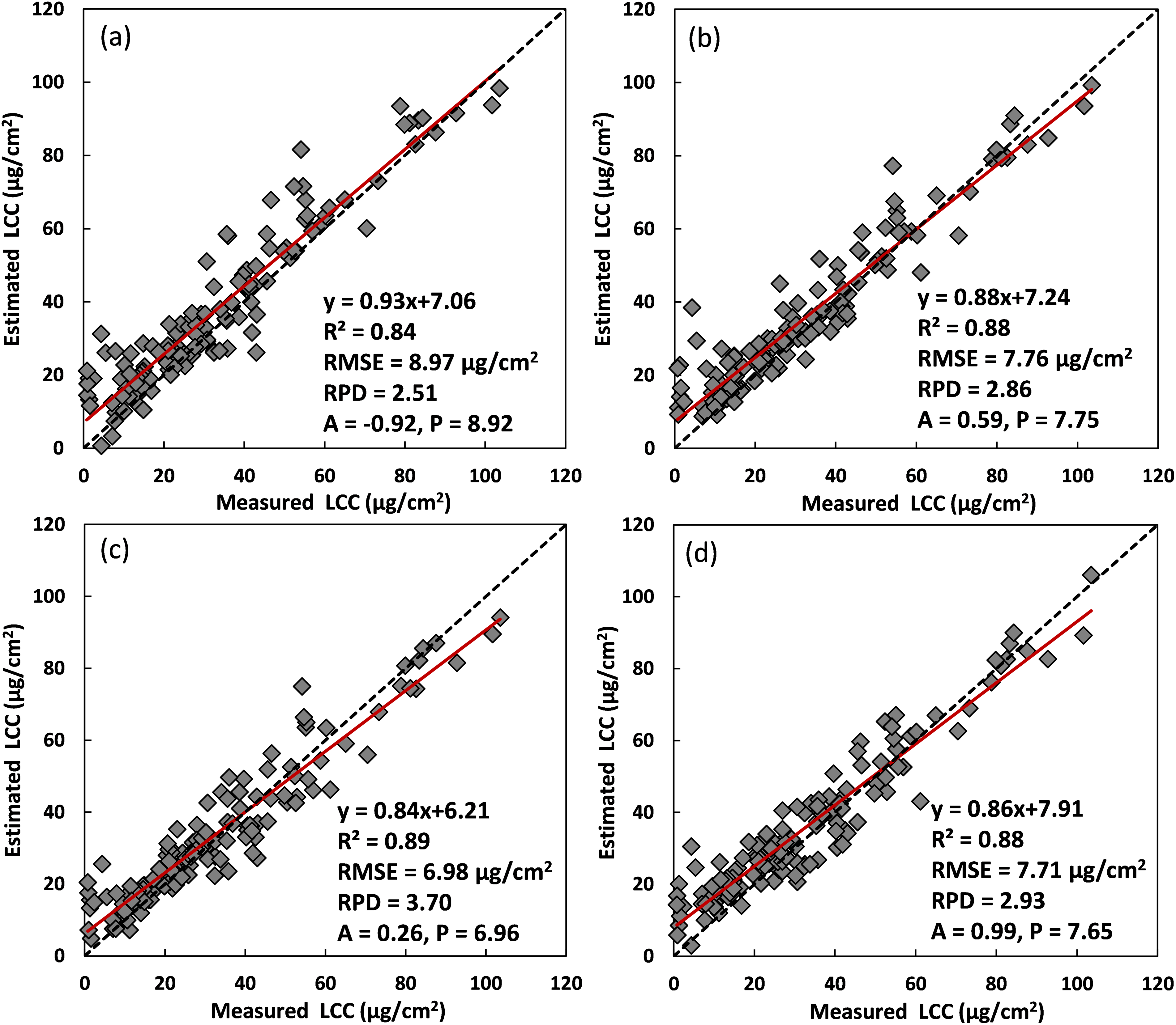
Figure 3: LCC validation results using ResNet-18 with different data sizes. (a)–(d) were results for a calibrated model combining the training part of ANGERS data with 200, 500, 800, and 1000 simulated data

Apart from the overall scatterplot between measured and predicted LCC using the validation part of ANGERS data (n = 138), validation results, with different ResNet-18 models using 200, 500, 800, and 1000 simulated data, were further analyzed based on four LCC value ranges (i.e., 0–20, 21–40, 41–60, 61–120), and new R2, RMSE, and RPD were calculated accordingly. Statistics results for these LCC value ranges are presented in Table 3, which shows that ResNet-18 models exhibited varied performance for different LCC value ranges. For LCC values in 0–20 μg/cm2 intervals, all models showed low accuracies with R2 values lower than 0.2. ResNet-18 model with 800 synthetic data behaved with a relatively low RMSE value of 7.35 than other models. For LCC values ranging from 21 to 40 μg/cm2, ResNet-18 models with 500 and 800 simulations showed slightly better estimation results than other models. Predicted LCC values in this range showed lower RMSE values, for ResNet-18 models with 500, 800 emulated data, than those values in Fig. 3a,d. For LCC values within 40–60 μg/cm2 range, best accuracies (R2 value around 0.6, RMSE value about 7.4 μg/cm2) were achieved by models with 500 and 1000 simulated datasets, while for LCC values larger than 60 μg/cm2, models with 200 and 500 emulations showed superior estimation results (R2 value around 0.7, RMSE value about 6.6 μg/cm2) than other models.

3.3 Feature Selection with ResNet-18 for LCC Estimation

Besides using reflectance in 400–1000 nm as input when training the ResNet-18 model, 15 spectral indices that were designed for chlorophyll retrieval, were considered as input features to investigate the feasibility of ResNet-18 for LCC estimation. In addition, a CARS algorithm was used to optimize spectral indices as input features, since these SIs were derived with four types of equations (Table 1) using reflectance from specific wavebands, which might encounter information redundancy issues. Results of CARS for feature selection using the ANGERS data (n = 276) are shown in Fig. 3. With the increase of iteration, the numbers of variables, i.e., spectral indices, exhibited a steady downward tendency (Fig. 4a). In comparison, the behavior of RMSECV showed obvious vibrations during the iteration process. When iteration values were larger than 40, RMSECV values behaved with a significant rising trend. The lowest RMSECV, when the iteration value was 15, was considered for determining the optimized quantity of spectral indices. 9 spectral indices, including RD2, PSSRa, RR710, RR720, NDVI, CIred edge, SIP, EPI, and mSR705, were then selected as in put features for further ResNet-18 modeling.

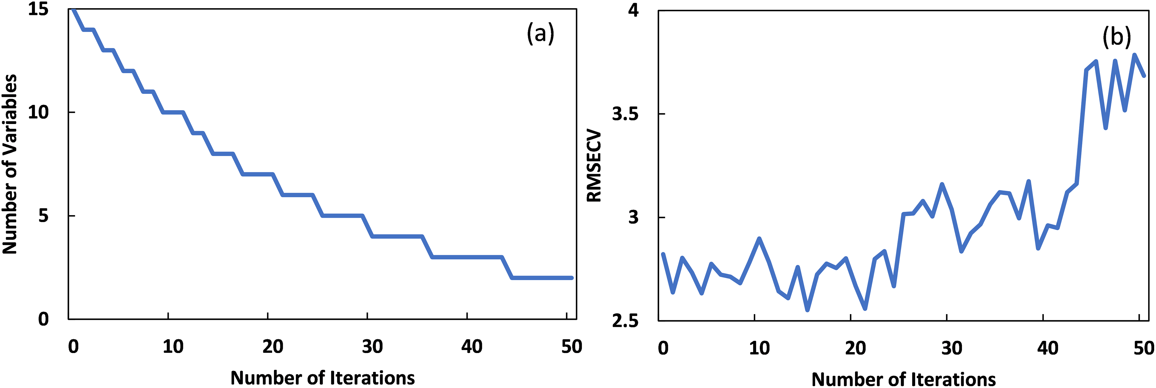
Figure 4: Results of CARS for feature selection. (a) was changing the trend of the number of SIs with the increase of iterations, (b) was RMSE variations when iterations increased

Based on the results of different data sizes for LCC retrieval in Fig. 3, 800 synthetic data combined with the training part of ANGERS data (Section 2.4) were used for ResNet-18 modeling with spectral indices as input features, on the consideration that ResNet-18 with 800 emulated data behaved with overall accurate estimation compared with other models. Validation results of these models with remanent ANGERS data are presented in Fig. 5. Compared with validation results in Fig. 3c that use reflectance from 400 to 1000 nm as input features, models with spectral indices exhibited superior estimation accuracies. Firstly, model evaluation indexes, such as fitted equations, R2, RRMSE, and RPD values for ResNet-18 with SIs were much more accurate than those using 400–1000 nm reflectance. Furthermore, estimated LCC values with SIs showed a more clustered distribution around a 1:1 line than that using reflectance (400–1000 nm) as input features. In addition, when LCC values were lower than 20 μg/cm2, ResNet-18 with SIs exhibited better sensitivity to LCC variations than that model using reflectance from 400–1000 nm. In terms of SIs selection for LCC modeling, ResNet-18 with the 9 selected SIs exhibited even better results than that using all the SIs: Scatterplot of estimated and measured LCC in Fig. 5b was more converged around 1:1 line, with the slope value (0.94) of the fitted line closer to 1. Moreover, LCC values larger than 80 μg/cm2 in Fig. 5a were underestimated than those in Fig. 5b.

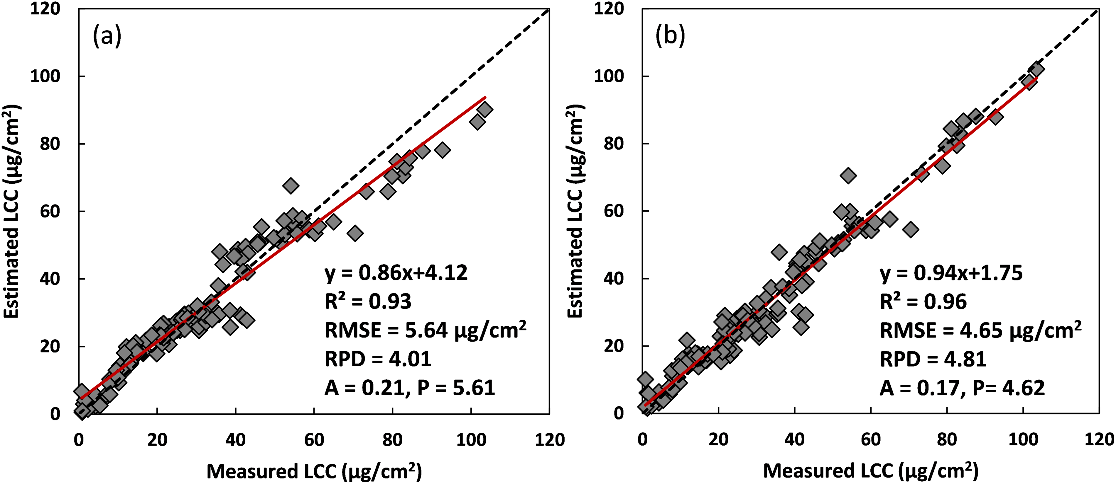
Figure 5: Validation results of SIs as input for LCC estimation with ResNet-18. (a) was the result using all 15 spectral indices, and (b) was the result with 9 SI features using CARS algorithm

3.4 Combining Transfer Learning with ResNet-18 for LCC Assessment

Based on the results of ResNet-18 with the selected 9 spectral indices as input features, a transfer learning method coupled with ResNet-18 (i.e., TL-ResNet-18) was used to investigate its performance of on LCC retrieval concerning convergence issues during model training, and its estimation accuracies were compared with only ResNet-18 modeling. Loss values, i.e., MSE, of the model training process for ResNet-18 and TL-ResNet-18 were then analyzed. Fig. 6a shows the convergence results of ResNet-18 training with the selected 9 spectral indices as input features using the calibration part of ANGERS data (n = 138). The initial loss value for ResNet-18 training was very large (approximated 1600), and then its values descended to 23, rapidly in the process of the first 28 iterations. With the advance of training sessions, loss values gradually reduced to 0.01 at 256 epochs. When iterations were about 400, a significant increase occurred to loss values, and its values were then lowered and flatted as the number of iterations increased to 1000. In comparison, the convergence process of TL-ResNet-18 with 800 simulated data for coarse tuning, and partially measured data (n = 138) for fine tuning was more stable and faster. Its initial loss value started from 53.53 and rapidly decreased to 0.01 at 152 epochs. Even though variations of loss values appeared from 345 (0.44) to 385 (0.61) iterations, overall loss values were no larger than 1.0. Moreover, its values were close to 0 after 400 iterations.

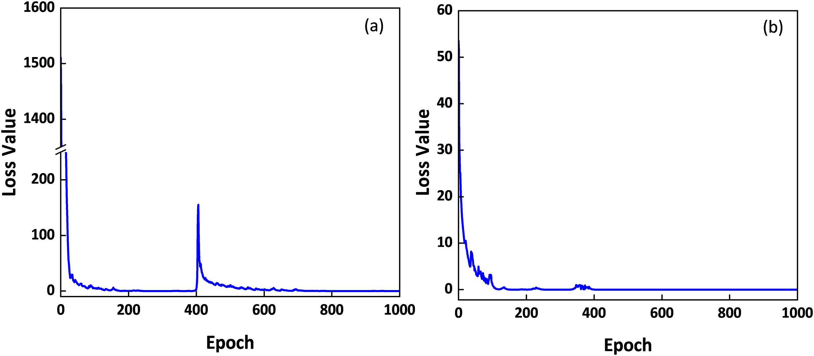
Figure 6: Convergence of losses for the model training process. (a) were results of ResNet-18 training with the selected 9 spectral indices as input features using the calibration part of ANGERS data, (b) resulted using TL-ResNet-18 with 800 simulated data for coarse tuning, and the calibration part of ANGERS data for fine-tuning

With these training results, validation of ResNet-18 and TL-ResNet-18 models using the same remanent ANGERS data (n = 138) are shown in Fig. 7. Results indicated that both ResNet-18 and TL-ResNet-18 exhibited good estimation accuracies for LCC retrieval, with an R2 value larger than 0.9, a RMSE value lower than 6.2 μg/cm2, and a RPD value higher than 4.0. Among these two models, TL-ResNet-18 behaved with slightly better validation results: the slope value of the fitted line (0.97) between measured and predicted LCC was closer to 1, and LCC values around 0 were better estimated than that by ResNet-18. Nevertheless, a sample with an LCC value of 60 μg/cm2 was obviously overestimated by both two models. Compared with results in Fig. 4b that using ResNet-18 combing 800 synthetic and partially measured data with the 9 selected spectral indices as input features, ResNet-18 modeling using only measured data (Fig. 6a) showed a slightly worse estimation result with an increase of 1.61 μg/cm2 for RMSE values and a decrease of 0.78 for RPD values. In terms of the TL-ResNet-18 model, its behavior in LCC estimation did not exceed those results in Fig. 5b as well.

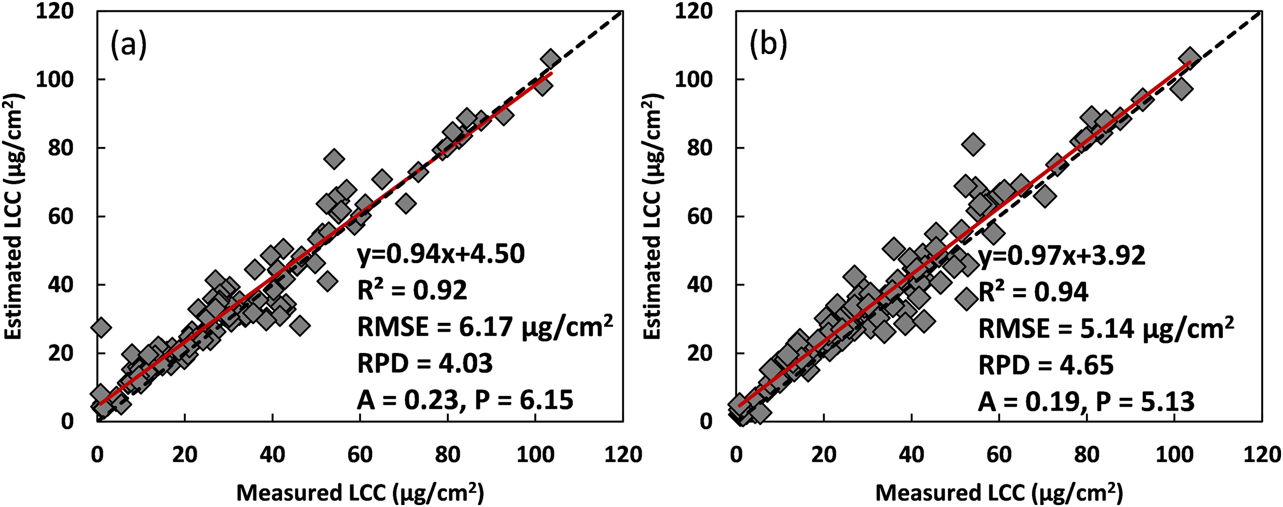
Figure 7: Validation results of the selected 9 SIs as input for LCC estimation. (a) were results for ResNet-18 using the ANGERS data, and (b) were results for TL-ResNet-18 using 800 synthetic data combined with the ANGERS dataset

4  Discussion

Accurate estimation of LCC is crucial to better know the process of material and energy exchange between plants and the environment. In the present study, the effects of adding synthetic data for modeling, input feature optimization, and model convergence issues for accurate and robust estimation of plant LCC with a deep learning framework (i.e., ResNet-18) were comprehensively investigated. In order to analyze the influence of data size on LCC assessment, a multi-output GPR algorithm was used, instead of leaf level RTM, such as PROSPECT series, to simulate abundant synthetic data, according to characteristics of the ANGERS dataset, for ResNet-18 model training process. Even though RTMs could simulate abundant reflectance data using different plant parameters as input, unrealistic combinations could still occur, which might lead to large differences from measured data, and thus affect model accuracies when using these invalid simulations, particularly for some situations using nonlinear models [3,37]. Moreover, differences between simulated data using RTMs and measured data could hardly be quantified, which might, in turn, deteriorate the modeling process. By contrast, 400–1000 nm reflectance simulation with the GPR model using ANGERS data showed satisfactory results: absolute and relative residual values, compared with corresponding measured reflectance from 400 to 1000 nm, were all around 0. Nevertheless, limit values of relative residual before 700 nm exhibited obvious variations, particularly for its minimum value at 680 nm. Reasons for this might largely be attributed to the insufficiency of the GPR algorithm for several simulations when corresponding measured reflectance possessed significant differences from general cases, just like measured reflectance with the red dot line in Fig. 2a. In addition, boundary values of relative residual values after 700 nm exhibited limited variations, suggesting the accurate ability of the GPR algorithm for simulation. Variations in absolute residual values further supported these views as well. These residual results were similar to the work conducted by Rivera et al. [20] using different ML methods for approaching RTM simulations. Which suggests the feasibility of applying statistics learning methods for synthetic data simulation.

According to LCC retrieval results with ANGERS and simulated data using raw reflectance, we found that adding a certain amount of simulated data for ResNet-18 training could increase model accuracies. Results in Fig. 3 and Table 3 suggested that the underestimation phenomenon of LCC values in the range of 0–20 μg/cm2 became less obvious, with the increase of simulated data for model training. Which suggested the feasibility of adding simulated data for ResNet-18 training. As for the amount of synthetic data used for the ResNet-18 modeling, 800 simulations were considered on account of model validation results in Fig. 3. Nevertheless, detailed estimation results for different LCC ranges in Table 3 showed that the ResNet-18 model combined partial ANGEERS data and 800 simulations did not outperform other models for all LCC value ranges. Reasons for this might be partially attributed to LCC distribution characteristics. Since validated ANGERS data exhibited a feature that 32% LCC values were lower than 20 μg/cm2 and 37% LCC values were in the 21–40 μg/cm2 range. ResNet-18 model training with measured ANGERS data and 800 simulations exhibited excellent accuracies in these two ranges than remanent ranges compared with other models. Thus, we suggest that adding synthetic data for CNN modeling should concern the similarity between measured data and simulation, and statistics features of target variables, to obtain accurate estimation. In terms of measured data partition when used for model training and testing, several attempts were considered when combining 800 simulations for model establishment. We found that varied dividing schemes had limited influence on estimation accuracies of ResNet-18 for LCC retrieval: with an R2 value of around 0.88, an RMSE value of about 7.0 μg/cm2, and an RPD value of approximately 3.5. Thus, an equal division of the ANGERS data was used for model calibration and validation.

Compared with using original reflectance from 400–1000 nm as input, ResNet-18 modeling with 15 spectral indices showed improved estimation accuracies in LCC retrieval, which suggests that SIs might be more suitable for LCC modeling. Moreover, estimated LCC with SIs features exhibited better convergence with measured LCC around a 1:1 line in comparison with those results using 400–1000 nm reflectance. This might be attributed to that spectral indexes that formed from different reflectance with varied formations were more sensitive to capture LCC variations than initial band reflectance, even if these two factors were used as inputs for convolution in ResNet-18 to obtain convolved features. This was particularly obvious when LCC values were lower than 20 μg/cm2 (or close to 0 μg/cm2), ResNet-18 with spectral indices exhibited much better estimations than that using 400–1000 nm reflectance. In addition, 15 spectral indices that were fed to ResNet-18 might be not the optimal features, since 9 spectral indices selected from CARS combined with ResNet-18 exhibited better estimation accuracies compared with that using 15 SIs. Furthermore, predicted LCC by ResNet-18 with 9 SIs showed better distribution vs. measured LCC. Apart from LCC values less than 20 μg/cm2 were accurately retrieved in both two situations (Fig. 5a,b), several LCC values in the 40–60 μg/cm2 range, were better estimated by ResNet-18 with 9 SIs. Moreover, LCC values larger than 80 μg/cm2 were obviously underestimated in comparison with those values in Fig. 5b. This could be to some extent explained by the decrease of input features dimension could filter out SIs with low weights after the CARS algorithm, and thus improve the estimation accuracies for LCC values higher than 80 μg/cm2. As for 9 chosen SIs by the CARS algorithm, band reflectance in these indices was mainly concentrated in 445, 505, 680, 700, 705, 710, 720, 740, 750, and 800 nm. Reflectance from these mentioned wavebands was mostly considered crucial information, especially for the red-edge region (700–780 nm), for crop agronomic parameter retrieval, such as chlorophyll [38], nitrogen [39], and leaf area index [40]. Apart from these selected indices, RD1, ND705, PRI, PSRI, CIgreen, and MTCI were not chosen by CARS. Even though some of these SIs are composed of red-edge reflectance as well, compared with selected SIs, these SIs might contain certain information redundancy and possess low weight when used in the CARS algorithm. Which could lead to no consideration of these SIs by CARS. These results indicate that combining feature optimization with ResNet-18 modeling using hyperspectral data could reduce model input dimension, and improve its efficiency while ensuring modeling accuracy, which was consistent with the results obtained by Zhang et al. [41].

Combining the transfer learning techniques could indeed improve the model convergence rate since the initial training loss value decreased from approximately 1600 to 53.53 when using TL-ResNet-18 for model training (Fig. 6). Moreover, it could help ResNet-18 to slightly increase LCC estimation accuracies in comparison with the results in Fig. 7a. These were accorded with the results of Wang et al. [15]. Even though overall results of TL-ResNet-18 model using the same 9 spectral indices exhibited a little inferior accuracy compared with results in Fig. 5b, scattered points of measured data vs. predicted LCC in Fig. 7b showed slightly better convergence around 1:1 line, especially for several sample points with LCC values close to 0 μg/cm2, and some with LCC values around 40 μg/cm2, which further suggested the effectiveness of TL-ResNet-18 for improving LCC estimation. Nevertheless, there were still some deficiencies in the present study. First, several simulations using the GPR algorithm with the ANGERS data characteristics exhibited significant differences with corresponding measured reflectance in 400–1000 nm, which could incur model estimation error. Moreover, considering that the total amount of ANGERS data was 276, the maximum amount of synthetic data was set to 1000, which might not be large enough compared with research using tens of thousands of simulations for CNN model training. In addition, SIs that were used as model input factors just included five different types, of abundant spectral indices that were proposed for chlorophyll retrieval still needed to be investigated to derive optimal input features for accurate and generalized CNN model establishment. In a word, the present study comprehensively evaluated the effects of synthetic data simulation, input feature optimization, and model convergence issue and generalization for accurate and robust estimation of plant LCC with ResNet-18, we suggested that TL-ResNet-18 could be used for improved LCC assessment using optimized SIs as input features, and this proposed a retrieval mode when CNN models were used for accurate agronomic parameters estimation, particularly with very limited measured data.

5  Conclusions

In this study, the effects of combining synthetic data for modeling, input feature optimization, and model convergence issues for accurate and robust estimation of plant LCC with the ResNet-18 framework were comprehensively evaluated. A multi-output GPR model was established based on the ANGERS data, and it exhibited good accuracies (an RMSE value of 0.04, an RRMSE value of 27.01%, and an NRMSE value of 12.77%) for 400–1000 nm reflectance data simulation. On the whole, adding synthetic data for ResNet-18 training could increase its estimation accuracies when raw reflectance from 400–1000 nm was used as model input. ResNet-18 training with 800 simulations and partial ANGERS data exhibited accurate results, with an R2 value of 0.89, an RMSE value of 6.98 μg/cm2, an RPD value of 3.70, for LCC retrieval using remanent ANGERS data. In comparison, ResNet-18 modeling with 9 spectral indexes, selected from the CARS algorithm, showed improved LCC estimation accuracies (an R2 value of 0.96, an RMSE value of 4.65 μg/cm2, an RPD value of 4.81). In addition, coupling transfer learning with ResNet-18 could boost the model convergence rate, and TL-ResNet-18 exhibited accurate results for LCC estimation (R2 = 0.94, RMSE = 5.14 μg/cm2, RPD = 4.65). These results suggest that adding appropriate synthetic data, input features optimization, and transfer learning techniques could be effectively used for improved LCC retrieval with a ResNet-18 model.

Acknowledgement: The authors would like to thank Jochem Verrelst for his support with the ARTMO toolbox. The authors would also like to thank the anonymous reviewers for providing comments that helped improve the quality of the original manuscript.

Funding Statement: This study was financially supported by the National Natural Science Foundation of China (Project Nos. 41901268 and 42371385), and Zhejiang Provincial Natural Science Foundation of China (Grant No. LTGN23D010002).

Author Contributions: The authors confirm their contribution to the paper as follows: study conception and design: Xianfeng Zhou and Ruiju Sun; data collection: Xianfeng Zhou and Zhaojie Zhang; analysis and interpretation of results: Xianfeng Zhou, Yuanyuan Song and Lin Yuan; draft manuscript preparation: Xianfeng Zhou, Lijiao Jin and Lin Yuan. All authors reviewed the results and approved the final version of the manuscript.

Availability of Data and Materials: The data that support the findings of this study are available from the corresponding author upon reasonable request.

Ethics Approval: Not applicable.

Conflicts of Interest: The authors declare no conflicts of interest to report regarding the present study.

References

1. Simkin AJ, Kapoor L, George Priya Doss C, Hofmann TA, Lawson T, Ramamoorthy S. The role of photosynthesis related pigments in light harvesting, photoprotection and enhancement of photosynthetic yield in planta. Photosynth Res. 2022;152(1):23–42. doi:10.1007/s11120-021-00892-6. [Google Scholar] [PubMed] [CrossRef]

2. Bhadra S, Sagan V, Maimaitijiang M, Maimaitiyiming M, Newcomb M, Shakoor N, et al. Quantifying leaf chlorophyll concentration of Sorghum from hyperspectral data using derivative Calculus and machine learning. Remote Sens. 2020;12(13):2082. doi:10.3390/rs12132082. [Google Scholar] [CrossRef]

3. Zhou X, Zhang J, Chen D, Huang Y, Kong W, Yuan L, et al. Assessment of leaf chlorophyll content models for winter wheat using Landsat-8 multispectral remote sensing data. Remote Sens. 2020;12(16):2574. doi:10.3390/rs12162574. [Google Scholar] [CrossRef]

4. Zhang J, He H, Fan D, Fu B, Wang S, Dong S. Research of chlorophyll-a concentration inversion at different depths in Hong Kong offshore waters based on Gaussian process regression. IOP Conf Ser: Earth Environ Sci. 2022;1087(1):012034. doi:10.1088/1755-1315/1087/1/012034. [Google Scholar] [CrossRef]

5. Tian H, Wang P, Tansey K, Han D, Zhang J, Zhang S, et al. A deep learning framework under attention mechanism for wheat yield estimation using remotely sensed indices in the Guanzhong Plain, PR China. Int J Appl Earth Obs Geoinf. 2021;102(6):102375. doi:10.1016/j.jag.2021.102375. [Google Scholar] [CrossRef]

6. Makantasis K, Karantzalos K, Doulamis A, Doulamis N. Deep supervised learning for hyperspectral data classification through convolutional neural networks. In: 2015 IEEE International Geoscience and Remote Sensing Symposium (IGARSS); 2015 Jul 26–31; Milan, Italy: IEEE; 2015. p. 4959–62. doi:10.1109/IGARSS.2015.7326945. [Google Scholar] [CrossRef]

7. Cunha RLF, Silva B, Netto MAS. A scalable machine learning system for pre-season agriculture yield forecast. In: IEEE 14th International Conference on e-Science (e-Science); 2018; Amsterdam, Netherlands: IEEE. p. 423–30. doi:10.1109/eScience.2018.00131. [Google Scholar] [CrossRef]

8. Barman U. Deep Convolutional neural network (CNN) in tea leaf chlorophyll estimation: a new direction of modern tea farming in Assam. India J Appl Nat Sci. 2021;13(3):1059–64. doi:10.31018/jans.v13i3.2892. [Google Scholar] [CrossRef]

9. Shi S, Xu L, Gong W, Chen B, Chen B, Qu F, et al. A convolution neural network for forest leaf chlorophyll and carotenoid estimation using hyperspectral reflectance. Int J Appl Earth Obs Geoinf. 2022;108(3):102719. doi:10.1016/j.jag.2022.102719. [Google Scholar] [CrossRef]

10. Zhou J, Zhou J, Ye H, Ali ML, Chen P, Nguyen HT. Yield estimation of soybean breeding lines under drought stress using unmanned aerial vehicle-based imagery and convolutional neural network. Biosyst Eng. 2021;204(5):90–103. doi:10.1016/j.biosystemseng.2021.01.017. [Google Scholar] [CrossRef]

11. Prilianti KR, Onggara IC, Adhiwibawa MAS, Brotosudarmo THP, Anam S, Suryanto A. Multispectral imaging and convolutional neural network for photosynthetic pigments prediction. In: 5th International Conference on Electrical Engineering, Computer Science and Informatics (EECSI); 2018; Malang, Indonesia: IEEE. p. 554–9. doi:10.1109/EECSI.2018.8752649. [Google Scholar] [CrossRef]

12. Elsherbiny O, Fan Y, Zhou L, Qiu Z. Fusion of feature selection methods and regression algorithms for predicting the canopy water content of rice based on hyperspectral data. Agriculture. 2021;11(1):51. doi:10.3390/agriculture11010051. [Google Scholar] [CrossRef]

13. Zhang J, Cheng T, Guo W, Xu X, Qiao H, Xie Y, et al. Leaf area index estimation model for UAV image hyperspectral data based on wavelength variable selection and machine learning methods. Plant Meth. 2021;17(1):49. doi:10.1186/s13007-021-00750-5. [Google Scholar] [PubMed] [CrossRef]

14. Bahrami H, Homayouni S, Safari A, Mirzaei S, Mahdianpari M, Reisi-Gahrouei O. Deep learning-based estimation of crop biophysical parameters using multi-source and multi-temporal remote sensing observations. Agronomy. 2021;11(7):1363. doi:10.3390/agronomy11071363. [Google Scholar] [CrossRef]

15. Wang D, Wang J. Crop disease classification with transfer learning and residual networks. Transact Chin Soc Agricul Eng (Transact CSAE). 2021;37(4):199–207. doi:10.11975/j.issn.1002-6819.2021.4.024. [Google Scholar] [CrossRef]

16. Malathi V, Gopinath MP. Classification of pest detection in paddy crop based on transfer learning approach. Acta Agric Scand Sect B. 2021;71(7):552–9. [Google Scholar]

17. Ye H, Tang S, Yang C. Deep learning for chlorophyll-a concentration retrieval: a case study for the Pearl River Estuary. Remote Sens. 2021;13(18):3717. doi:10.3390/rs13183717. [Google Scholar] [CrossRef]

18. Liu P, Shi R, Zhang C, Zeng Y, Wang J, Tao Z, et al. Integrating multiple vegetation indices via an artificial neural network model for estimating the leaf chlorophyll content of Spartina alterniflora under interspecies competition. Environ Monit Assess. 2017;189(11):596. doi:10.1007/s10661-017-6323-6. [Google Scholar] [PubMed] [CrossRef]

19. Feret JB, François C, Asner GP, Gitelson AA, Martin RE, Bidel LPR, et al. PROSPECT-4 and 5: advances in the leaf optical properties model separating photosynthetic pigments. Remote Sens Environ. 2008;112(6):3030–43. doi:10.1016/j.rse.2008.02.012. [Google Scholar] [CrossRef]

20. Rivera J, Verrelst J, Gómez-Dans J, Muñoz-Marí J, Moreno J, Camps-Valls G. An emulator toolbox to approximate radiative transfer models with statistical learning. Remote Sens. 2015;7(7):9347–70. doi:10.3390/rs70709347. [Google Scholar] [CrossRef]

21. Yu K, Lenz-Wiedemann V, Chen X, Bareth G. Estimating leaf chlorophyll of barley at different growth stages using spectral indices to reduce soil background and canopy structure effects. ISPRS J Photogramm Remote Sens. 2014;97(3):58–77. doi:10.1016/j.isprsjprs.2014.08.005. [Google Scholar] [CrossRef]

22. Tucker CJ. Red and photographic infrared linear combinations for monitoring vegetation. Remote Sens Environ. 1979;8(2):127–50. doi:10.1016/0034-4257(79)90013-0. [Google Scholar] [CrossRef]

23. Lemaire G, Jeuffroy M, Gastal F. Diagnosis tool for plant and crop N status in vegetative stage: theory and practices for crop N management. Eur J Agron. 2008;28(4):614–24. doi:10.1016/j.eja.2008.01.005. [Google Scholar] [CrossRef]

24. Blackburn GA. Quantifying chlorophylls and caroteniods at leaf and canopy scales an evaluation of some hyperspectral approaches. Remote Sens Environ. 1998;66(3):273–85. doi:10.1016/S0034-4257(98)00059-5. [Google Scholar] [CrossRef]

25. Zarco-Tejada PJ, Miller JR, Noland TL, Mohammed GH, Sampson PH. Scaling-up and model inversion methods with narrowband optical indices for chlorophyll content estimation in closed forest canopies with hyperspectral data. IEEE Trans Geosci Remote Sens. 2001;39(7):1491–507. doi:10.1109/36.934080. [Google Scholar] [CrossRef]

26. Vogelmann JE, Rock BN, Moss DM. Red edge spectral measurements from sugar maple leaves. Int J Remote Sens. 1993;14(8):1563–75. doi:10.1080/01431169308953986. [Google Scholar] [CrossRef]

27. Rouse JW, Haas RH, Deering DW, Schell JA, Harlan JC. Monitoring the vernal advancement and retrogradation (green wave effect) of natural vegetation. In: Contractor report. Greenbelt, MD, USA: NASA/GSFC; 1974. [Google Scholar]

28. Gitelson A, Merzlyak MN. Spectral reflectance changes associated with autumn senescence of Aesculus hippocastanum L. and Acer platanoides L. leaves. spectral features and relation to chlorophyll estimation. J Plant Physiol. 1994;143(3):286–92. doi:10.1016/S0176-1617(11)81633-0. [Google Scholar] [CrossRef]

29. Gamon JA, Peñuelas J, Field CB. A narrow-waveband spectral index that tracks diurnal changes in photosynthetic efficiency. Remote Sens Environ. 1992;41(1):35–44. doi:10.1016/0034-4257(92)90059-S. [Google Scholar] [CrossRef]

30. Merzlyak MN, Gitelson AA, Chivkunova OB, Rakitin VY. Non-destructive optical detection of pigment changes during leaf senescence and fruit ripening. Physiol Plant. 1999;106(1):135–41. doi:10.1034/j.1399-3054.1999.106119.x. [Google Scholar] [CrossRef]

31. Gitelson AA, Gritz Y, Merzlyak MN. Relationships between leaf chlorophyll content and spectral reflectance and algorithms for non-destructive chlorophyll assessment in higher plant leaves. J Plant Physiol. 2003;160(3):271–82. doi:10.1078/0176-1617-00887. [Google Scholar] [PubMed] [CrossRef]

32. Peñuelas J, Baret F, Filella I. Semi-empirical indices to assess carotenoids/chlorophyll a ratio from leaf spectral reflectance. J Appl Geophy. 1995;31(2):221–30. [Google Scholar]

33. Datt B. Remote sensing of chlorophyll a, chlorophyll b, chlorophyll a + b, and total carotenoid content in Eucalyptus leaves. Remote Sens Environ. 1998;66(2):111–21. doi:10.1016/S0034-4257(98)00046-7. [Google Scholar] [CrossRef]

34. Sims DA, Gamon JA. Relationships between leaf pigment content and spectral reflectance across a wide range of species, leaf structures and developmental stages. Remote Sens Environ. 2002;81(2–3):337–54. doi:10.1016/S0034-4257(02)00010-X. [Google Scholar] [CrossRef]

35. Dash J, Curran PJ. The MERIS terrestrial chlorophyll index. Int J Remote Sens. 2004;25(23):5403–13. doi:10.1080/0143116042000274015. [Google Scholar] [CrossRef]

36. Fernandes R, Brown L, Canisius F, Dash J, He L, Hong G, et al. Validation of Simplified Level 2 Prototype Processor Sentinel-2 fraction of canopy cover, fraction of absorbed photosynthetically active radiation and leaf area index products over North American forests. Remote Sens Environ. 2023;293(2):113600. doi:10.1016/j.rse.2023.113600. [Google Scholar] [CrossRef]

37. Combal B, Baret F, Weiss M, Trubuil A, Macé D, Pragnère A, et al. Retrieval of canopy biophysical variables from bidirectional reflectance Using prior information to solve the ill-posed inverse problem. Remote Sens Environ. 2003;84(1):1–15. doi:10.1016/S0034-4257(02)00035-4. [Google Scholar] [CrossRef]

38. Zhou X, Zhang J, Wu K, Chen D, Ma H, Huang W, et al. A digital sensor with non-imaging multi-spectral and image modules for continuous monitoring of plant growth conditions: development and validation. Comput Electron Agric. 2024;225(10):109299. doi:10.1016/j.compag.2024.109299. [Google Scholar] [CrossRef]

39. Schlemmer M, Gitelson A, Schepers J, Ferguson R, Peng Y, Shanahan J, et al. Remote estimation of nitrogen and chlorophyll contents in maize at leaf and canopy levels. Int J Appl Earth Obs Geoinf. 2013;25(9):47–54. doi:10.1016/j.jag.2013.04.003. [Google Scholar] [CrossRef]

40. Herrmann I, Pimstein A, Karnieli A, Cohen Y, Alchanatis V, Bonfil DJ. LAI assessment of wheat and potato crops by VENμS and Sentinel-2 bands. Remote Sens Environ. 2011;115(8):2141–51. doi:10.1016/j.rse.2011.04.018. [Google Scholar] [CrossRef]

41. Zhang Y, Hui J, Qin Q, Sun Y, Zhang T, Sun H, et al. Transfer-learning-based approach for leaf chlorophyll content estimation of winter wheat from hyperspectral data. Remote Sens Environ. 2021;267:112724. doi:10.1016/j.rse.2021.112724. [Google Scholar] [CrossRef]