Fault Diagnosis Method of Rolling Bearing Based on ESGMD-CC and AFSA-ELM

1  Introduction

Rolling bearing is commonly applied in industrial production and other environments, and is extremely important to equipment operation. The study of rolling bearing working conditions and its fault diagnosis method is helpful to improve the stability of equipment and prevent the occurrence of serious equipment failure [1,2]. The usual to maintain the operating status of a rolling bearing is to obtain vibration signals by an accelerometer. In steady working conditions, the characteristics of its vibration signal are without large changes, but by the complex working and environmental conditions, its operation may be due to improper assembly, overload, insufficient lubrication, and other reasons [3,4], gradually appear wear, corrosion, and in serious cases even damage failure and other abnormal defeat. Subsequently, the amplitude of the vibration signal will also gradually increase.

Bearing fault signal is often non-stationary and interspersed with noise, and the key to diagnosis is to extract the fault characteristic frequency from the modulated vibration signal. Processing the fault signal through signal processing techniques can reduce the influence of noise interference, and it is beneficial to identify the fault type and severity, further improve the accuracy of fault diagnosis. The commonly used methods include wavelet transform [5], Fourier transform [6], Wigner-Ville distribution [7], and other various signal decomposition methods. Zhang et al. [8], based on the quaternion Fourier transform and empirical wavelet transform, proposed a multichannel signal processing method of QEWT, and combined with spectral negentropy, which was successfully applied to the field of fault diagnosis. Liu et al. [9] proposed a bearing fault diagnosis method based on CEEMD and LDWPSO-PNN, which improved the signal decomposition performance of the EMD-based method and enhanced the accuracy of fault classification, while the optimized diagnosis performance was verified in the comparison methods. Wang et al. [10] proposed a theory based on adaptive parameters optimized VMD to improve the decomposition performance of rolling bearing by introducing the spectrum degree of cross-correlation which is the criterion of selecting the optimal penalty factor.

Due to more vibration sources, complex transmission paths and strong noise interference. It is usually difficult to accurately extract the periodic shock sequence caused by local damage to the bearing through the above signal processing methods. Aiming at the improvement of characteristics extraction in rolling bearing fault signals, Pan et al. [11] proposed the SGMD method which is capable of adaptive decomposition. SGMD has the advantages of keeping the inherent features of the time series unchanged, suppressing the modal aliasing, and is suitable for handling mechanical fault vibration signals. However, there are also theoretical and practical issues to improve, such as reconstruction constraints, defects in decomposition errors, etc.

After the proposed enhanced ESGMD-CC method, the decomposed components contain a large amount of fault-related information. However, a suitable strategy is still needed to extract fault features from these decomposed components. Various strategies have been developed by scholars to cope with it. Ye et al. [12], by extracting the multiscale permutation entropy of VMD components, effectively bridged the signal decomposition method and classifier to improve the performance of fault classification. Chen et al. [13] calculated the energy entropy in order to effectively input the IMFs of CEEMDAN into the LSSVM classifier, and achieved better diagnostic results. Zhang et al. [14] designed a bearing fault diagnosis method based on WPD and optimized RBF, and verified the effectiveness of the method by extracting the reconstructed components of WPD through energy features and inputting them into the classifier. However, these methods have a certain degree of computational complexity and need to be further dealt with without taking into account the quantity of some redundant components.

After feature extraction, suitable classification algorithms need to be utilized to discover various potential faults of rolling bearing in time, and a lot of research has been carried out by domestic and foreign scholars in machine learning and other aspects. Commonly used methods generally include Back Propagation (BP), Random Forest (RF), Support Vector Machine (SVM), Extreme Learning Machine (ELM), etc., which are implemented by mapping and matching fault features to classification labels [15–18]. Xiao et al. [19] proposed a fault diagnosis model with a beetle-optimized BP neural network, which can find the error extremes faster, shorten the training time, and have some anti-interference capability. Wan et al. [20], proposed an improved RF to eliminate redundant decision trees by filtering the RF, parallel retention and constructing a decision tree similarity matrix, which is effective for fault classification of rolling bearings. Zhang et al. [21], in order to improve the classification performance of the model, proposed a fault detection method based on MPE and SOA-SVM, which accurately accomplishes the identification of faults by taking the MPE matrix features decomposed by VMD and inputting them into the SVM model optimized by the seagull optimization algorithm. From the above studies, it can be found that these classification algorithms, with many parameter settings, extreme values and slow training speed, limit the application in fault diagnosis.

ELM is a class of single hidden layer feedforward neural networks with fast learning speed and high generalization ability, which is suitable for application in fault diagnosis. Xi et al. [22] proposed a feature extraction model based on wavelet decomposition and weighted PE to effectively extract feature vectors and input them into an ELM model with optimal parameters for classification, and achieved better test accuracy. The stability and accuracy of fault diagnosis will be impacted by the ELM’s random setting of weights and bias. As a result, an appropriate method must be introduced for optimization to prevent the impact of random selection on the outcomes of the diagnosis.

To address the above problems, a fault diagnosis integrating with enhanced ESGMD-CC and AFSA-ELM is proposed in this paper, and technique route is shown in Fig. 1. Firstly, SGMD decomposes the raw signal into SGCs. Secondly, the iterations are reset by the cosine difference limitation to effectively separate the redundant components from the representative components. Additionally, the calculus operator is performed to strengthen weak fault features and make them easier to extract, and the singular values weighted by PSE are utilized as the sample feature representation. Finally, AFSA iteratively optimized ELM is adopted as the optimized classifier for fault identification.

Figure 1: The technical route of this paper

The rest of this paper is organized as follows. Section 2 mainly introduces methods of signal decomposition and feature extraction. Section 3 describes the establishment of classifier. Section 4 introduces the experimental arrangement and the corresponding analyzes. Section 5 summarizes this paper.

2  Signal Decomposition and Feature Extraction

2.1 The Traditional SGMD Theory

As a new mode decomposition method, the advantage of SGMD is that the Symplectic transform can preserve the phase space of the system structure. The SGMD method obtains the Hamilton matrix by reconstructing the phase space of the one-dimensional vibration signal, and then solves the eigenvalues and eigenvectors of the Hamilton matrix by the Symplectic transform, and finally reconstructs the SGCs by diagonal averaging.

(1) Phase space reconstruction

Let x=x1,x2,⋯,xn and project x onto the trajectory matrix X according to Takens embedding theorem, as follows:

X=[x1x1+τ⋯x1+(d−1)τ:::xmxm+τ⋯xm+(d−1)τ] (1)

where d is the embedding dimension; m=n−(d−1)τ ; τ is the delay time. In order to construct X reasonably, d is selected based on the power spectral density (PSD) of the original vibration signal [23].

(2) QR decomposition

Let A=XTX , then the Hamilton matrix is as follows:

M=(A00−AT) (2)

Let F=M2 , then the matrix F is also a Hamiltonian matrix, through Symplectic orthogonal matrix Q , we can get:

QTFQ=(BR0BT) (3)

where B is an upper triangular matrix with the eigenvalues λ1,λ2,⋯,λd , so the eigenvalues of matrix A are σi=λi(i=1,2,⋯d) , and its corresponding eigenvectors are Qi(i=1,2,⋯,d) . The reconstructed trajectory matrix Z is constructed from a series of initial single component matrices Zi(i=1,2,⋯,d) as follows:

Z=Z1+Z2+⋯+Zd (4)

where Zi=QiSi , Si=QiTXT .

(3) Diagonal averaging transformation

For the element zij(1≤i≤m,1≤j≤d) in matrix Zi , let m∗=max(m,d) . If m<d , let zij∗=zij , otherwise, zij∗=zji .

Then the diagonal averaging transformation is shown in Eq. (5):

yk={1k∑p=1kzp,k−p+1∗1≤k<d∗1d∗∑p=1d∗zp,k−p+1∗d∗≤k≤m∗1n−k+1∑p=k−m∗+1n−m∗+1zp,k−p+1∗m∗<k≤n (5)

By diagonal averaging transformation, the initial matrix Zi can be converted into Yi(y1,y2,⋯,yn) :

Y=Y1+Y2+⋯+Yd (6)

2.2 ESGMD-CC Theory

The SGMD theory yields a number of initial single components Y , which often includes redundant components. It is crucial to distinguish the representative components from the redundant components [24]. The cosine difference limitation is used in this situation to successfully reset the iterations and separate the redundant components. The eigenvectors that correspond to relatively large eigenvalues in the signal also contain redundant components, necessitating further processing. The calculus operator is also introduced to make weak fault characteristics more easily extractable and to avoid weak fault features from being obscured by background noise.

(1) Separation of redundant components by cosine difference limitation

First, sum the decomposed SGCs. For the obtained Y , the sum components Sk can be obtained as follows:

Sk=∑i=1kYi (7)

Second, cosine the adjacent sum components. For the obtained Sk , calculate their cosine values Cosi according to Eq. (8):

Cosi=cos⁡(Sk,Sk+1)=Sk⋅Sk+1‖Sk‖⋅‖Sk+1‖ (8)

Finally, obtain the difference limitation. Combined with the characteristics of Cosi , the difference limitation can be more helpful to find the turning point accurately where the sum components achieve to be consistent. The cosine difference limitation CDi is constructed by Eq. (9):

CDi=|(Cosi+1−Cosi)|<εe (9)

when the values of CDi change steadily and reach the pre-set value εe which tends to zero, the former z can be chosen as the representative components. Before the z point, it contains plenty of helpful information of the raw signal. After the z point, it can be donated as redundant parts.

Finally, the raw signal x is composed of

x=∑i=1zYi+rz (10)

rz=∑i=z+1dYi (11)

where rz is the sum of the redundant components after the turning point z .

(2) Signal enhancement by calculus operator

Research [25] has shown that differential and integral signals can improve fault characteristics. To fully profit from these, calculus operator is used to the processing of signal components. The relevance is that it is possible to boost high-frequency featured components, lessen low-frequency redundant components, and emphasize transitory components by calculus operator. This strengthens weak fault characteristics and makes them easier to extract.

The differential result of the discrete signal Y(n) in shown in Eq. (12):

D(Y(n))=(Y(n)−Y(n−1))/Δt (12)

where Δt=1/fs , and fs is the sampling frequency.

The integral result of the discrete signal Y(n) in shown in Eq. (13):

I(Y(n))=ΔT(Y(n)+Y(n−ΔT))/2 (13)

where ΔT is the step factor. If it is set to 1, Eq. (13) can be simplified as follows:

I(Y(n))=(Y(n)+Y(n−1))/2 (14)

By integrating the differential and integral equations, the calculus operator of discrete signal Y(n) can be expressed as follows:

ca(Y(n))=I(D(Y(n)))=I(Y(n)−Y(n−1))=(Y(n)−Y(n−2))/2 (15)

For the reserved first z groups SGCs, the calculus operator is adopted for signal enhancement, which can fully amplificated the advantages of differential and integral. To simplify the calculation, Δt and ΔT in Eqs. (12) and (13) are both set to 1, so the ESLCs is shown as follows:

ESLCi=ca(Yi(n))=(Yi(n)−Yi(n−2))/2 (16)

ESGMD-CC is a robust and adaptive signal decomposition technique with targeted improvement that can handle processing fault signals with background noise and weak fault characteristics.

2.3 Feature Extraction by Weighted SVD

A number of ESLCs with a variety of fault-related data may be available by the aforementioned ESGMD-CC. An appropriate method is still required to extract fault characteristics from these obtained ESLCs. These fault characteristics can be successfully extracted by SVD, which also properly shows the fault-related feature information. It is suitable for ESLCs-based matrix’s feature extraction. The power spectrum entropy, which might display the uncertainty of the signal, simultaneously measures the feature vectors. The steps are as follows:

(1) The proposed ESGMD-CC is firstly applied to decompose the raw signals into ESLCs with hi(t) .

(2) SVD is utilized on hi(t) to obtain the singular values matrix Vi :

Vi=SVD([h1(t),h2(t),…,hh(t)]T) (17)

(3) Fourier transform hi(t)=(hi1,hi2,…,hin) to obtain Fi(fr) on frequency domain, where fr is a spectrum, then the power spectrum Pi(fr) is:

Pi(fr)=12πn|Fi(fr)|2 (18)

According to Parseval’s theorem, energy is invariable in the transfer stage from two domains related to time and frequency [26], so it can be written as:

|∑j=1nhij|2=|∑r=1nPi(r)|2 (19)

The power spectrum entropy PSi can be donated as:

Ei=−∑r=1nHirln⁡Hir (20)

where Hir is the proportion of the r−th power spectrum component in hi(t) , and its calculation is as follows:

Hir=Pi(r)/∑r=1nPi(r) (21)

(4) The weighted matrix Wi is as follows:

{g=Emax−EminWi=Ei−Eming (22)

The weighted singular values Ri can be obtained as follows:

Ri=Wi×Vi(i=1,2,…,h) (23)

The overall flowchart of signal decomposition and feature extraction is shown in Fig. 2.

Figure 2: The overall flowchart of signal decomposition and feature extraction

3  The Establishment of the AFSA-ELM Classifier

In this section, the ELM model and AFSA theory are initially explained firstly for the AFSA-ELM classifier. The choice of the random parameters in the fundamental ELM model has a significant influence on the generalization performance and diagnostic precision of fault diagnosis. In order to plan the best course of action and find the globally optimal solutions, AFSA is capable of optimizing the random parameters for each artificial fish. It then builds the AFSA-ELM model to enhance the performance of the classifier.

3.1 The Basic ELM Model

ELM is a feedforward neural network with only one hidden layer, and its generalization performance is better than that of traditional neural network models, and only the number of hidden layer neurons needs to be set without adjusting its parameters to obtain the solution during the training process. The structure of ELM is shown in Fig. 3. The specific process is as follows:

Figure 3: The structure of ELM

For the ELM network structure with an input sample X , the number of nodes in the hidden layer l , the output function Y can be expressed as follows:

Y=∑ilβig(WXj+b),j=1,2,…,N (24)

where W is the input weight, i.e., the connection weight between the input layer and the hidden layer; β is the output weight, i.e., the connection weight before the hidden layer and the output layer; b is the bias of the hidden layer; and g(x) is the activation function.

The neural network is trained so that the error is minimized, i.e., the error between the output and the desired output is close to 0, the error can be calculated as follows:

|Y−T|=0 (25)

Combining Eqs. (24) and (25) to obtain:

∑ilβig(WXj+b)=T,j=1,2,…,N (26)

Simplifying the above expression Eq. (26) as follows:

Hβ=T′ (27)

where H is the output matrix of the hidden layer nodes; T is the expected output.

The lowest training error may theoretically be attained by ELM. Just the number of neurons must be taken into account while employing ELM for pattern recognition. The stability and accuracy of fault detection will be impacted since the input weight and bias are produced by functions, which have a degree of unpredictability. It must utilize a proper algorithm to optimize the basic ELM.

3.2 AFSA-ELM Classifier

AFSA is a new intelligent algorithm by simulating fish swarm, which can rely on the field of view to adjust its position during foraging, and mainly contains the behaviors of searching, swarming, chasing and random, etc., gradually expanding from local to global to obtain the global optimal solution [27], and its main behaviors are described as follows:

(1) AF-search

The AF realizes external perception by its vision:

Xj=Xi+V⋅R(−1,1) (28)

where Xi is the current state of the i−th artificial fish, Xj is the position after moving, V is the field of view, and R(−1,1) is a random value between −1 and 1.

Xit+1=Xi1+Xi−XitXj−Xit⋅S⋅R(−1,1) (29)

where Xit+1 is the state of the artificial fish after the t+1 iteration and S is the step size.

(2) AF-swarm

The number of artificial fish in the visual range is nf , and their average position is Xa , if Ya/nf>δYi , where δ is the crowding factor, indicating a high food concentration at this position, then a move of step S is performed:

XC=∑i=1nfXinf (30)

Xit+1=Xi1+Xa−Xit||Xa−Xit||⋅ S⋅R(−1,1) (31)

(3) AF-chase

The individual with the best state in the current visual field Xj has a food concentration of Yj , if it satisfies Yj/nf>δYi , indicating that Yj is highest at Xj . The other individuals move towards Xj in steps S :

Xit+1=Xi1+Xj−Xit||Xj−Xit||⋅ S⋅R(−1,1) (32)

(4) AF-random

If the iteration reaches the maximum number of iterations Gmax , Yj is still not satisfied, then a randomly selected position in the current field of view is chosen and a step S is moved towards that state:

Xit+1=Xit+V⋅R(−1,1) (33)

The parameters that may be chosen during ELM training are insufficient to address the demands of diagnosis performance because of the low stability of ELM. The artificially set input weights and hidden layer bias of the ELM model, which are typically assigned by random calculation functions, is a significant factor in the instability of the ELM prediction results. The input weights and hidden layer bias thus obtained might not be suitable for fault classification. AFSA-ELM was constructed to improve the performance of the classifier. The flow chart of the AFSA-ELM is shown in Fig. 4, and the steps of constructing the AFSA-ELM are as follows:

Figure 4: The flow chart of the AFSA-ELM

Step 1: The ELM single hidden layer neural network structure is constructed and the input weights and hidden layer bias are initialized.

Step 2: The input weights and hidden layer bias are passed to the individual locations of artificial fish in AFSA, the relationship between them is established, and the sample data are input into the AFSA-ELM.

Step 3: An iterative operation is performed, containing search, swarm, chase and random behavior. When the termination condition of the AFSA algorithm is satisfied, the optimal artificial fish individual positions in the current AFSA dataset are transferred to the ELM, i.e., the optimal input weights and hidden layer bias available to the current ELM.

Step 4: At the completion of each iteration, determine whether Gmax is reached, and if so, output the optimal solution, and if not, return to Step 3.

Step 5: The optimal parameters are transferred to ELM to obtain the fault diagnosis classifier and test it accordingly.

4  Experiment Validation

To assess the efficacy of the proposed method in this study, two distinct datasets are chosen for validation, which contain CWRU and HFZZ, and they will be covered in depth subsequently.

4.1 Experiment Platform and Data Description

The CWRU rolling bearing experimental platform is shown in Fig. 5. The accelerometers with sampling frequency of 12 KHz are attached to the motor drive end and the fan end, respectively to collect fault signals in various states, and the detailed data chosen for this section are shown in Table 1, where each fault includes 1024 sampling points, and there is no overlap between them.

Figure 5: The CWRU experimental platform

The HFZZ rotating machinery fault diagnosis simulation platform is shown in Fig. 6. The bearing model is N205. Four kinds of faults were available for experiments through the IEPE accelerometer with the sampling frequency of 12.8 KHz installed on the bearing housing. The physical diagram and time domain waveform of the faults are depicted in Figs. 7 and 8, respectively.

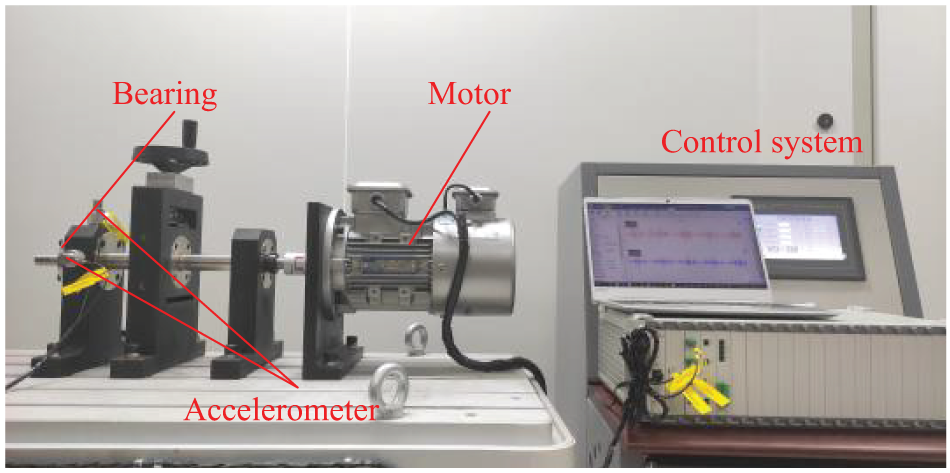
Figure 6: The HFZZ experimental setup

Figure 7: The four rolling bearings from HFZZ

Figure 8: The time domain waveform obtained from HFZZ

4.2 Experiment Setup

After data preprocessing, no distinctive features could be observed based on the time domain waveform of the rolling bearing, so the proposed method needs to be applied for further fault identification. The relevant comparative tests are carried out in this part from the following angles in order to fully assess the performance demonstrated by the proposed method. In the aforementioned trials, 10 separate experiments were carried out for each group to eliminate bias, and additional comparative items, including the average accuracy, were afterwards listed.

(1) The improved ESGMD-CC is combined with weighted SVD feature extraction to assess the benefits of the overall feature extraction method. It is then compared to EEMD, LMD, and VMD, and to the traditional SGMD method to assess the necessity of the proposed constraints based on the cosine difference limitation and calculus operator.

(2) The AFSA optimized ELM classification model is compared to the basic ELM model and to a number of other methods, like BP, SVM, etc., in order to demonstrate the benefits of the optimized classifier.

(3) The proposed fault diagnosis method is compared with some work published in the literatures to evaluate the performance of the whole fault diagnosis process.

4.3 Experiment Results and Comparative Analysis

The first set of comparison tests was carried out to assess the necessity of introducing cosine difference limits and calculus operator limitations by contrasting the improved ESGMD-CC with the conventional SGMD. A set of vibration signals under the inner race defect are shown in Fig. 9 as the first four SGCs, the last four SGCs, and the improved first four ESLCs, respectively. As can be observed, the energy is distributed more evenly throughout the first four SGCs while their amplitudes are less. The iterations may also be limited by the cosine difference limitation constraint, which also lowers the dimensionality by efficiently distinguishing superfluous components from representative components. Calculus operators have the advantage of enhancing the fault features in the signal.

Figure 9: The decomposed components by ESGMD-CC

Also, EEMD, LMD and VMD were compared with the improved ESGMD-CC. The weighted SVD mapping was employer in the feature extraction stage, and the AFSA-ELM classification algorithm was utilized to output the diagnostic results. The feature vectors produced by the various approaches outlined above were visualized by t-SNE, as shown in Fig. 10. Although it is evident that the various approaches produce various clustering effects, the precise accuracy of the classification cannot be determined only from Fig. 10. The associated experimental findings are presented in Table 2 and Fig. 11.

Figure 10: Feature mapping by t-SNE

Figure 11: The diagnosis results by different feature extraction methods

It is evident that the enhanced ESGMD-CC outperforms numerous others in terms of diagnostic performance. This is primarily caused by the fact that all ESLCs are capable of improving the fault characteristics of the signal as well as reducing the feature dimension while retaining representative components and deleting superfluous ones in the signal processing. The enhanced ESGMD-CC has more decomposed modes than some other signal decomposition techniques, but less than the traditional SGMD. The enhanced ESGMD-CC can successfully assess and rebuild the pre-existing modes in the original signal while preserving the phase space’s organization, and the fault information is richer and more detailed in the decomposed ESLCs.

Then, a second set of comparison experiments evaluated the benefit of the classifier and the AFSA optimization. The function of AFSA in the proposed AFSA-ELM classifier is to iteratively seek for the best parameters in the ELM model in order to improve diagnostic outcomes. As two widely used classification models, BP and SVM are included in the comparison. The results are shown in Table 3 and Fig. 12.

Figure 12: The diagnosis results by different classifiers

According to the above results, it can be seen that in most experiments, after the feature extraction algorithm proposed in this paper and then the fault identification by the classifier, the diagnosis accuracy of the ELM is generally higher than that of other models, and even more outstanding after AFSA-optimized ELM parameters. In the AFSA-ELM fault diagnosis model, the input weights and bias are precise based on the prediction errors on the training set to ensure that the two parameters of the ELM model are optimized, while the output weights are further adjusted based on the above two parameters to achieve structural optimization and parameter preference of the AFSA-ELM, which converges to the optimal solution faster and better, and thus has better diagnosis accuracy.

Several literature also used the CWRU rolling bearing dataset, even if other research also employed alternate open-source or independently developed datasets for testing. In order to further prove the efficacy of the proposed strategy, comparisons between the available literatures were made during the third set of experiments, as shown in Table 4. Although the accuracy of the techniques presented varies, they all have high accuracy, the testing accuracy of the proposed approach is higher than that of other ways. In comparison to the shallow optimization feature extraction and classification techniques in [28], the updated feature extraction and classification algorithms are more accurate. The enhanced feature extraction approach and iterative optimization classification model provided in this study should work together quite effectively. In order to get better diagnostic results, the literature [29] used a deep network that uses one-dimensional convolutional neural networks. Its diagnostic performance is on par with the well-designed deep network using the techniques described in this research in terms of diagnostic accuracy.

5  Conclusion

In order to explore an effective rolling bearing defect detection method, the enhanced ESGMD-CC and the AFSA-ELM are provided in this paper. The proposed method first utilizes the SGMD to decompose the raw signal into numerous SGCs, and then the cosine difference limitation and the calculus operator served as limiting constraints are introduced to reconstruct the SGCs into ESLCs. Then, fault characteristics are extracted from the obtained ESLCs by weighted SVD, which are then supplied to the following classifier for fault identification. Finally, the parameters of the ELM are iteratively found for optimality by the AFSA to construct the optimized classifier for fault identification. On the bearing dataset, pertinent comparison tests were carried out to confirm the diagnostic effectiveness of the proposed method and it is a promising method in the field of fault diagnosis. Extraction of characteristics from signals in complex noise environments and increasing approach efficiency will be key entry points in the future.

Acknowledgement: None.

Funding Statement: This work was supported by National Key Research and Development Project (2020YFE0204900), National Natural Science Foundation of China (Grant Numbers 62073193, 61873333), and Key Research and Development Plan of Shandong Province (Grant Numbers 2019TSLH0301, 2021CXGC010204).

Author Contributions: The authors confirm contribution to the paper as follows: study conception and design: Jiajie He, Fuzheng Liu, Faye Zhang; data collection: Fuzheng Liu; analysis and interpretation of results: Jiajie He, Xiangyi Geng, Mingshun Jiang; draft manuscript preparation: Jiajie He, Xifeng Liang. All authors reviewed the results and approved the final version of the manuscript.

Availability of Data and Materials: The authors confirm that the data supporting the findings of this study are available within the article.

Conflicts of Interest: The authors declare that they have no conflicts of interest to report regarding the present study.

References

1. Pang, B., Nazari, M., Tang, G. (2022). Recursive variational mode extraction and its application in rolling bearing fault diagnosis. Mechanical Systems and Signal Processing, 165, 108321. [Google Scholar]

2. Pan, H., Xu, H., Zheng, J., Su, J., Tong, J. (2022). Multi-class fuzzy support matrix machine for classification in roller bearing fault diagnosis. Advanced Engineering Informatics, 51, 101445. [Google Scholar]

3. Zhou, J., Xiao, M., Niu, Y., Ji, G. (2022). Rolling bearing fault diagnosis based on WGWOA-VMD-SVM. Sensors, 22(16), 6281. [Google Scholar] [PubMed]

4. Zhuang, Z., Tao, H., Chen, Y., Stojanovic, V., Paszke, W. (2023). An optimal iterative learning control approach for linear systems with nonuniform trial lengths under input constraints. IEEE Transactions on Systems, Man, and Cybernetics: Systems, 53(6), 3461–3473. https://doi.org/10.1109/TSMC.2022.3225381 [Google Scholar] [CrossRef]

5. Tao, H., Qiu, J., Chen, Y., Stojanovic, V., Cheng, L. (2023). Unsupervised cross-domain rolling bearing fault diagnosis based on time-frequency information fusion. Journal of the Franklin Institute, 360(2), 1454–1477. [Google Scholar]

6. Tao, H., Wang, P., Chen, Y., Stojanovic, V., Yang, H. (2020). An unsupervised fault diagnosis method for rolling bearing using STFT and generative neural networks. Journal of the Franklin Institute, 357(11), 7286–7307. [Google Scholar]

7. Singru, P., Krishnakumar, V., Natarajan, D., Raizada, A. (2018). Bearing failure prediction using Wigner-Ville distribution, modified Poincare mapping and fast Fourier transform. Journal of Vibroengineering, 20(1), 127–137. [Google Scholar]

8. Zhang, K., Deng, Y., Chen, P., Ma, C., Xu, Y. (2022). Quaternion empirical wavelet transform and its applications in rolling bearing fault diagnosis. Measurement, 195(8), 111179. [Google Scholar]

9. Liu, F., Gao, J., Liu, H. (2020). The feature extraction and diagnosis of rolling bearing based on CEEMD and LDWPSO-PNN. IEEE Access, 8, 19810–19819. [Google Scholar]

10. Wang, J., Zhang, Y., Zhang, F., Li, W., Lv, S. et al. (2021). Accuracy-improved bearing fault diagnosis method based on AVMD theory and AWPSO-ELM model. Measurement, 181(1–3), 109666. [Google Scholar]

11. Pan, H., Yang, Y., Li, X., Zheng, J., Cheng, J. (2019). Symplectic geometry mode decomposition and its application to rotating machinery compound fault diagnosis. Mechanical Systems and Signal Processing, 114(3), 189–211. [Google Scholar]

12. Ye, M., Yan, X., Jia, M. (2021). Rolling bearing fault diagnosis based on VMD-MPE and PSO-SVM. Entropy, 23(6), 762. [Google Scholar] [PubMed]

13. Chen, W., Li, J., Wang, Q., Han, K. (2021). Fault feature extraction and diagnosis of rolling bearings based on wavelet thresholding denoising with CEEMDAN energy entropy and PSO-LSSVM. Measurement, 172(6), 108901. [Google Scholar]

14. Zhang, Q., Gao, J., Dong, H., Mao, Y. (2018). WPD and DE/BBO-RBFNN for solution of rolling bearing fault diagnosis. Neurocomputing, 312(2), 27–33. [Google Scholar]

15. Xiao, M., Liao, Y., Bartos, P., Filip, M., Geng, G. et al. (2022). Fault diagnosis of rolling bearing based on back propagation neural network optimized by cuckoo search algorithm. Multimedia Tools and Applications, 81(2), 1–21. [Google Scholar]

16. Liu, A., Yang, Z., Li, H., Wang, C., Liu, X. (2022). Intelligent diagnosis of rolling element bearing based on refined composite multiscale reverse dispersion entropy and random forest. Sensors, 22(5), 2046. [Google Scholar] [PubMed]

17. Yang, K., Zhao, L., Wang, C. (2022). A new intelligent bearing fault diagnosis model based on triplet network and SVM. Scientific Reports, 12(1), 5234. [Google Scholar] [PubMed]

18. Liu, F., Wang, H., Li, W., Zhang, F., Zhang, L. et al. (2023). Fault diagnosis of rolling bearing combining improved AWSGMD-CP and ACO-ELM model. Measurement, 209(7), 112531. [Google Scholar]

19. Xiao, M., Zhang, W., Wen, K., Zhu, Y., Yiliyasi, Y. (2021). Fault diagnosis based on BP neural network optimized by beetle algorithm. Chinese Journal of Mechanical Engineering, 34(1), 1–10. [Google Scholar]

20. Wan, L., Gong, K., Zhang, G., Yuan, X., Li, C. et al. (2021). An efficient rolling bearing fault diagnosis method based on spark and improved random forest algorithm. IEEE Access, 9, 37866–37882. [Google Scholar]

21. Zhang, X., Wang, H., Ren, M., He, M., Jin, L. (2022). Rolling bearing fault diagnosis based on multiscale permutation entropy and SOA-SVM. Machines, 10(6), 485. [Google Scholar]

22. Xi, C., Gao, Z. (2022). Fault diagnosis of rolling bearings based on WPE by wavelet decomposition and ELM. Entropy, 24(10), 1423. [Google Scholar] [PubMed]

23. Bonizzi, P., Karel, J. M., Meste, O., Peeters, R. L. (2014). Singular spectrum decomposition: A new method for time series decomposition. Advances in Adaptive Data Analysis, 6(4), 1450011. [Google Scholar]

24. Li, H., Li, F., Jia, R., Zhai, F., Bai, L. et al. (2021). Research on the fault feature extraction of rolling bearings based on SGMD-CS and the AdaBoost framework. Energies, 14(6), 1555. [Google Scholar]

25. Cheng, Z., Wang, R. (2020). Enhanced symplectic characteristics mode decomposition method and its application in fault diagnosis of rolling bearing. Measurement, 166, 108108. [Google Scholar]

26. Zheng, Z., Xin, G. (2019). Fault feature extraction of hydraulic pumps based on symplectic geometry mode decomposition and power spectral entropy. Entropy, 21(5), 476. [Google Scholar] [PubMed]

27. Kou, Z., Yang, F., Wu, J., Li, T. (2020). Application of ICEEMDAN energy entropy and AFSA-SVM for fault diagnosis of hoist sheave bearing. Entropy, 22(12), 1347. [Google Scholar] [PubMed]

28. Zhang, X., Li, C., Wang, X., Wu, H. (2021). A novel fault diagnosis procedure based on improved symplectic geometry mode decomposition and optimized SVM. Measurement, 173, 108644. [Google Scholar]

29. Li, Y., Zou, L., Jiang, L., Zhou, X. (2019). Fault diagnosis of rotating machinery based on combination of deep belief network and one-dimensional convolutional neural network. IEEE Access, 7, 165710–165723. [Google Scholar]

30. Gu, Y., Zeng, L., Qiu, G. (2020). Bearing fault diagnosis with varying conditions using angular domain resampling technology, SDP and DCNN. Measurement, 156(11), 107616. [Google Scholar]