Intelligent Fault Diagnosis Method of Rolling Bearings Based on Transfer Residual Swin Transformer with Shifted Windows

1  Introduction

With the development of industrialization, rotating machinery is widely employed in many industrial fields, including petrochemical, power generation, transportation, and other industries [1]. Rolling bearings are crucial components in rotating machinery, which may be damaged and malfunctions under harsh working conditions [2,3]. Once a local defect occurs in the race, it would cause unexpected injuries and economic losses over time [4]. Thus, accurate and timely identification of bearing faults warrants the safe operation of mechanical equipment.

Generally speaking, fault diagnosis techniques include four parts, i.e., signal-based, model-based, knowledge-based, and hybrid/active methods [5]. The past few years have witnessed the widespread application of condition-monitoring systems, greatly promoting the knowledge-based method [6,7]. Machine learning is a typical response of knowledge-based methods in which decision-making trees, naive Bayes, and K-nearest neighbors (KNN) are widely used in practical applications. The fault diagnosis methods using machine learning mainly consist of three procedures, i.e., collecting data, extracting features, and identifying faults [8,9]. Soualhi et al. [10] proposed six elements to represent the working state of the motor bearing, and then fed the selected sensitive features into the neural network for fault classification. Prieto et al. [11] figured up 15 time-domain statistical parameters that present bearing health, and then selected features via discriminant analysis, utilizing an artificial neural network for fault classification. Boukra et al. [12] obtained time-frequency features and used an artificial neural network for fault classification. Soualhi et al. [13] applied the Hilbert-Huang transform to extract metrics from vibration signals and used a support vector machine to identify bearing faults. Dong et al. [14] used fuzzy C-means and KNN to complete the task of bearing fault diagnosis. However, fault diagnosis methods using machine learning require the prior knowledge of experts in the process of feature extraction, which is not an easy task. With the continuous increase of the amount of fault data, traditional machine learning gradually cannot meet the demand due to its low generalization performance, which also reduces the accuracy of fault diagnosis.

Recently, deep learning (DL), an important branch of machine learning has made great progress in many fileds, such as objective detection [15] and natural language processing (NLP) [16], and so on. Because the DL model can automatically learn features from the original vibration signal without manual selection, DL shows its advantages. In fault diagnosis, some DL methods have been used, for example, deep autoencoders, deep belief network (DBN), and convolutional neural networks (CNN). The DL model has the characteristics of extracting robust and recognizable features from high-dimensional structures. Sun et al. [17] proposed a sparse stacked network (SSN) for motor fault diagnosis. It is used to model the sparsity of the output labels and solve the SSN using kernel tricks. Gan et al. [18] applied a new hierarchical diagnosis network automatic diagnosis system, which mainly consists of DBN. Zhao et al. [19] presented a novel method based on gated recurrent unit networks, which learns representations of sequences of local features. Zhao et al. [20] developed a fault diagnosis method that used two-dimensional grayscale images and LeNet-5. Shao et al. [21] developed a multi-signal motor fault diagnosis method, in which the acquired sensor signals were converted to a wavelet time-frequency diagram (TFD) by wavelet transform (WT), and CNN was used to identify the fault. Wang et al. [22] designed a new method using joint learning for intelligent fault diagnosis. Shi et al. [23] developed a novel DL fault diagnosis method based on bidirectional-convolutional long short term memory networks for planetary gearbox. Liang et al. [24] proposed a fault diagnosis method for gearboxes using multi-label CNN and WT. Chen et al. [25] used CNN and discrete WT for fault recognition of planetary gearbox. Xu et al. [26] developed a global contextual multiscale fusion network, which can diagnose mechanical equipment in noisy and unbalanced scenarios. Chang et al. [27] proposed a network based on a dynamic selection mechanism, which allows the kernel to change the acceptance domain based on multi-scale information and complete fault diagnosis tasks in slow and sharp speed variations scenarios. To achieve ideal fault diagnosis performance under heavy noise, Han et al. [28] designed a network that integrates global and local information.

Although methods based on DL have received a lot of attention, there are still some problems with these methods. Since the labeled data samples in fault diagnosis are small, many DL models are barely more than five layers deep, which limits the final diagnosis. The deepening of the hidden layer will increase the free parameters, and training large networks from the beginning usually relies on a large amount of labeled data. Compared to large CNN models applied to the ImageNet dataset, the structure of DL model in the fault diagnosis field is relatively shallow. More importantly, it is not easy to train a deep CNN model without a dataset like ImageNet with tens of millions of labeled data.

Transfer learning (TL) attempts to overcome the problem of insufficient labeled data. TL can use network parameters trained on sufficiently labeled data from different application domains, which avoids random initialization of network parameters. In the fault diagnosis field, TL is developing very rapidly [29]. Wen et al. [30] used a sparse autoencoder to learn common features under different working conditions. Shao et al. [31] created a deep TL fault diagnosis method using WT and deep CNN. Xu et al. [32] proposed a novel transfer online CNN framework. Zhao et al. [33] created a multiscale convolutional TL network.

The transformer model [34] proposed by Google Brain has acquired great spectacular success in the NLP field. Dosovitaskiy et al. [35] created a vision Transformer (Vit) which directly used the standard transformer structure to image classification. Swin Transformer [36] used the shifted window self-attention, which retains the characteristic of locality and hierarchy of CNN. Swin Transformer has excellent global feature and local feature extraction ability.

Based on the above, a novel deep transfer residual Swin Transformer (RST), which used residual self-attention mechanism (RSA). A novel end-to-end method based on transfer RST is created for fault diagnosis. Firstly, our method converts the original vibration signal into a wavelet TFD, and then uses transfer RST to extract fault features from the wavelet TFD. The RST model has 24 layers of self-attention layers. At the same time, the parameters pre-trained on the ImageNet dataset are utilized, which enables RST to have reasonable initialization.

The contributions of this study are summarized as follows:

1) A new deep transfer RST is proposed to obtain fault features, which loads pre-trained parameters from the ImageNet dataset.

2) A new end-to-end method for fault diagnosis based on deep transfer RST and WT is proposed. The advantages of our approach are demonstrated on public datasets and self-built datasets.

The rest of the paper is organized as follows. Section 2 introduces the theoretical background of the proposed approach, including WT, Transformer, and Transfer learning. Section 3 shows details of RST. Section 4 presents the procedure of the proposed method for fault diagnosis. Section 5 shows the results of the proposed method on two datasets. Section 6 describes the conclusion.

2  Theoretical Background

2.1 WT

WT is a signal processing method that utilizes a variable width function to produce a range of resolutions, which is utilized for feature extraction in fault diagnosis. WT can subdivide time and frequency at high frequency and low frequency respectively, and it has the function of adaptively analyzing time-frequency signal. The meaning of WT is a certain wave is called a basic wavelet or mother wavelet. After the function ϕ(t) is shifted by τ , it makes inner product with the signal x(t) to be analyzed at different scales a:

WTx=1a∫−∞+∞x(t)ϕ(t−τa)dt,a>0 (1)

where a is the scale factor, τ is displacement. The scaling factor a can make the scaling transform of the basic wavelet ϕ(t) . If a becomes larger, it ϕ(ta) becomes wider. The signal becomes the wavelet TFD after WT.

The TFD essentially reflects the energy intensity of the signal at different times and frequencies. Wavelet TFD can reveal the detailed changes of the signal, so as to virtually display the slight fault feature of the signal. Compared to the 1-D vibration signal, it contains the time-frequency representations.

2.2 Transformer

Fig. 1 shows the transformer encoder’s structure, which is suitable for tasks such as machine translation. The encoder block consists of four parts, i.e., embedded and positional encoding layer, multi head self-attention (MSA) layer, residual connection layer and layer normalization (LN) layer [37,38], and feed-forward layer (FFN).

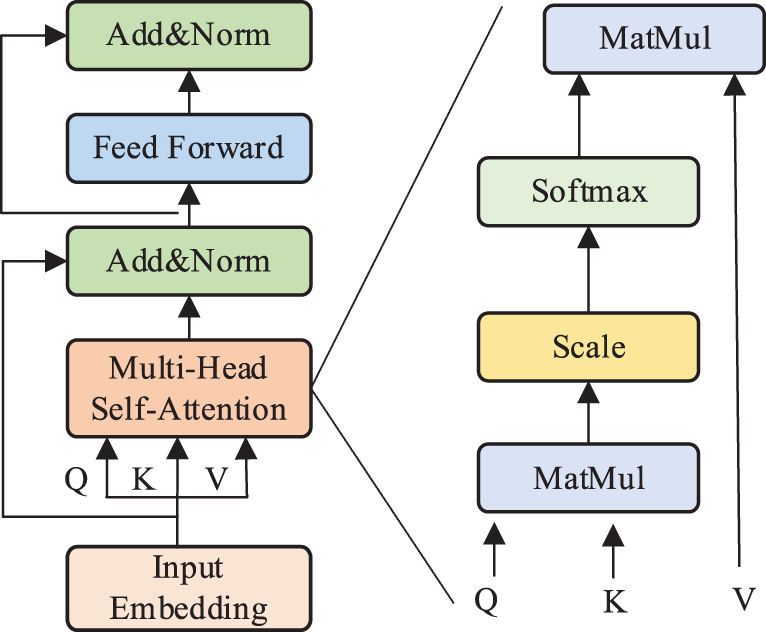
Figure 1: Structure of the transformer encoder

2.2.1 Embedded Layer

The embedded layer is responsible for encoding the input sequence into an embedded vector. The position vector of all words is obtained by positional encoding, which provides the position information of each comment to identify each word’s order relationship. The word vector and the position vector, which have the same dimension, are added to get the accurate vector representation of the word. The vector of the word is written as xt . All word vectors form a word vector matrix X .

2.2.2 Multi Head Self-Attention Layer

Its function is to learn a weight for each word of the input vector. Three matrices of WQ , WK and WV are defined here, and all word vectors are linearly transformed by these three matrices. The query matrix Q is composed of all qt vectors, the key matrix K is composed of all kt vectors, and the value matrix V is composed of all vt vectors.

The calculation method of attention utilizes scaled dot-product. It can be expressed as:

Attention(Q,K,V)=softmax(QKTdk)V (2)

where dk is the number of columns of the Q , K matrix.

MSA consists of multiple self-attention layers. The linear transformation matrix changes from one group to another, and finally concatenates the output of group h , the dimension of the matrix obtained is the same as the dimension of the input matrix X .

MSA can be denoted as:

Ah(X)=concat(head1,⋯,headh)WO (3)

headi=Attention(XWiQ,XWiK,XWiV) (4)

where WiQ∈Rdmod el×dQ , WiK∈Rdmod el×dK , WiV∈Rdmod el×dv represent i -th independent query/key/value weight matrix, which is multiplied by the embedded matrix X to get the Q K V matrix. WO∈Rh⋅dv×dmod el denotes the weight matrix, which concatenates all attention heads.

2.2.3 Residual Connection and LN Layer

The residual layer’s function is solving the degradation problem in DL. Normalizing the activation values of each layer and accelerating convergence are LN’s purposes. The residual connection layer and normalization layer can be demonstrated as follows:

XA=Layernorm(X+Attentionh(X)) (5)

2.2.4 FFN

Two fully connected (FC) layers form the FFN. ReLU is the activation function of the first layer, and the second layer has no activation function. The feed forward layer can be expressed as:

FF(X)=ReLU(0,XW1+b1)W2+b2 (6)

where Wc1∈Rdmod el×dff , Wc2∈Rdmod el×dcla , bc1∈Rdff , bc2∈RNcla is the weights and bias of a two-layer FC network.

2.3 Transfer Learning

The shared properties in these two domains can be transferred due to inherent similarities in different application scenarios or working conditions. The purpose of TL is to transfering the knowledge learned from the source domain to the target domain. TL can take advantage of training model parameters in the source domain so that the target domain deep learning model does not need random initialization.

In practice, the parameters of large deep learning models are randomly initialized before training and updated during training. This will limit the performance of deep learning models if the labeled data used for training is limited. TL is a promising solution to the problem of insufficient labeled data. TL can achieve desirable results using models pre-trained on large datasets and then trained on smaller datasets in other domains. The Swin Transformer model is first trained on the Imagenet dataset in this research.

3  Details of Residual Swin Transformer

3.1 Overview of RST

Fig. 2 presents RST’s structure. RST includes a patch partition model and four stages. Each stage is composed of an unequal number of RST blocks. RST block is constructed by a residual self-attention mechanism based on shifted windows.

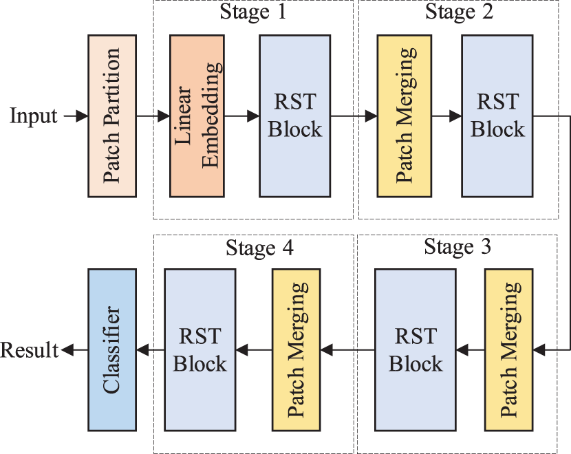
Figure 2: Structure of the RST

3.2 Patch Partition

The patch partition layer segments the wavelet time-frequency map into disjoint patches. Patches will be referred to as a token. The patch size is 4 × 4. The RGB channel of each pixel in the patch is expanded. The feature dimension of each token will be 4 × 4 × 3 = 48. Here, the token is recorded as z0 . The linear embedding layer maps the input token to features of any dimension C .

3.3 Linear Embedding and Patch Merging

To form a hierarchical representation, the token’s number needs to decrease as the layers’ number increases. The patch merging layer performs a splicing operation on the 2 × 2 size of the adjacent patch word depth channel, and then the set dimension size is obtained after the mapping change: H8×W8×2C . The patch merge operation for Stage 3 and Stage 4 has not changed from Phase 2. The dimensions of the patch become H32×W32×8C .

3.4 RST block

The multi-head residual self-attention (MRSA) module based on shifted windows replaces the standard MSA module in the RST block. Fig. 3 displays the structure of the RST block. An RST block is composed of the MRSA module and a two multi-layer perceptron (MLP). The LN layer follows the MRSA and MLP layers.

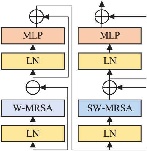
Figure 3: Architecture of two successive RST blocks

z~l=W−MRSA(LN(zl−1))+zl−1zl=MLP(LN(z~l))+z~lz~l+1=SW−MRSA(LN(zl))+zlzl+1=MLP(LN(z~l+1))+z~l+1 (7)

where z~l represents the W-MRSA and SW-MRSA’s output features and zl represents the MLP’s output features in block, respectively. On the one hand, W-MRSA adopts the conventional MRSA mechanism; on the other hand, SW-MRSA adopts the MRSA of shifted window partition.

If each window-based RSA module lacks the connection between windows, it will limit its modeling ability. RST adopts a shifted window partition method, and the two partition methods appear alternately in the RST block. Because the shift window division method connects adjacent non-overlapping windows, it has advantages in image classification.

Fig. 4 shows the shift window mechanism. No overlap and shifted window attention are on the left and right respectively. The shifted window includes the components of the original adjacent window. In practice, moving feature maps and constructing masks are used indirectly. It can keep the original number of windows unchanged. The self-attention calculation in the new window spans the boundaries of the previous windows in layer l, providing connections between them. Specifically, Fig. 5 demonstrates that the proposed model employs a circular shift to the upper left. Then, several non-adjacent sub-windows on the feature map constitute a batch window, so the self-attention computation is restricted on all sub-window by the masking mechanism. The cyclic shift can make batch processing windows’ numbers consistent with the regular window division. The gray areas A, B, and C have been moved to the black areas A, B, and C. Then perform MASK operations on the moved A, B, and C regions, as these regions are not related to the original regions. Next, perform RSA calculations. After completing the above operation, the ABC area is restored to its original position.

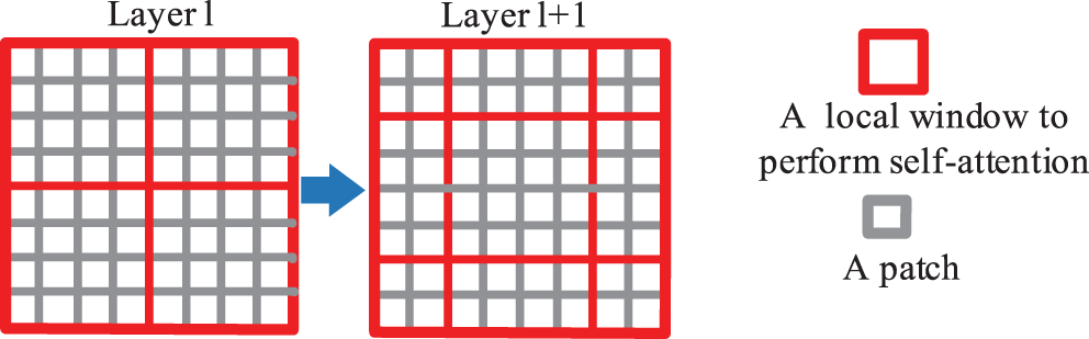
Figure 4: Descriptions of computation approach for window partitioning

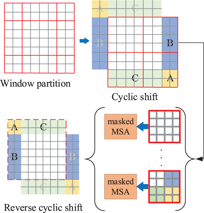
Figure 5: Descriptions of the shifted window approach for computing self-attention

RST adopts relative position bias, B∈RM2×M2 . RST utilizes the following formula to calculate the similarity:

Attention(Q,K,V)=softmax(QKT)/d+B)V (8)

where Q, K, V represents query, key and value matrices; d represents the query, key dimension, M2 represents the number of patches in a window.

RSA combines attention and input using residual connections to get the information of different weights in the sequences. RSA can be calculated as follows:

RSA(X,Q,K,V)=softmax(QKTdk+B)V+X (9)

3.5 Classifier

The classifier layer is divided into two layers: FFN and softmax. The output of softmax is the normalized probability of each classification.

CLA(z)=softmax(GeLU(zWc1+bc1)Wc2+bc2) (10)

GeLU(x)=0.5x(1+tanh(2/π(x+0.044715x3))) (11)

where bc1∈Rdff , bc2∈RNcla , Wc1∈Rdmodel×dff , Wc2∈Rdmodel×dcla are the biases and weights of the two layers. Ncla is the number of categories. dff is dimensions hidden layer.

3.6 Training of RST

In the process of training the RST model, this study uses the cross-entropy (CE) loss function. The Adam optimizer has been modified and upgraded from the previous optimizer. When computing the update step size, the first and second moment estimates of the gradient are taken into account. Adam optimizer has the advantages of high computational efficiency, low memory overhead, automatic adjustment of learning rate, and is not affected by gradient scaling. Given a training set G = {xi,yi}i=1n containing n samples, the model uses the CE loss function.

J(θ)=1n∑i=1nℓCE(yi,y^i) (12)

where yi and y^i are the true label and predicted label of the sample xi , respectively. ℓCE denotes the CE loss function and θ denotes the trainable parameters of RST.

4  The Implementation Steps of the Our Method

Our method automatically extracts the raw vibration signal’s fault features, which directly classify fault categories. Fig. 6 denotes the framework, and the steps are shown:

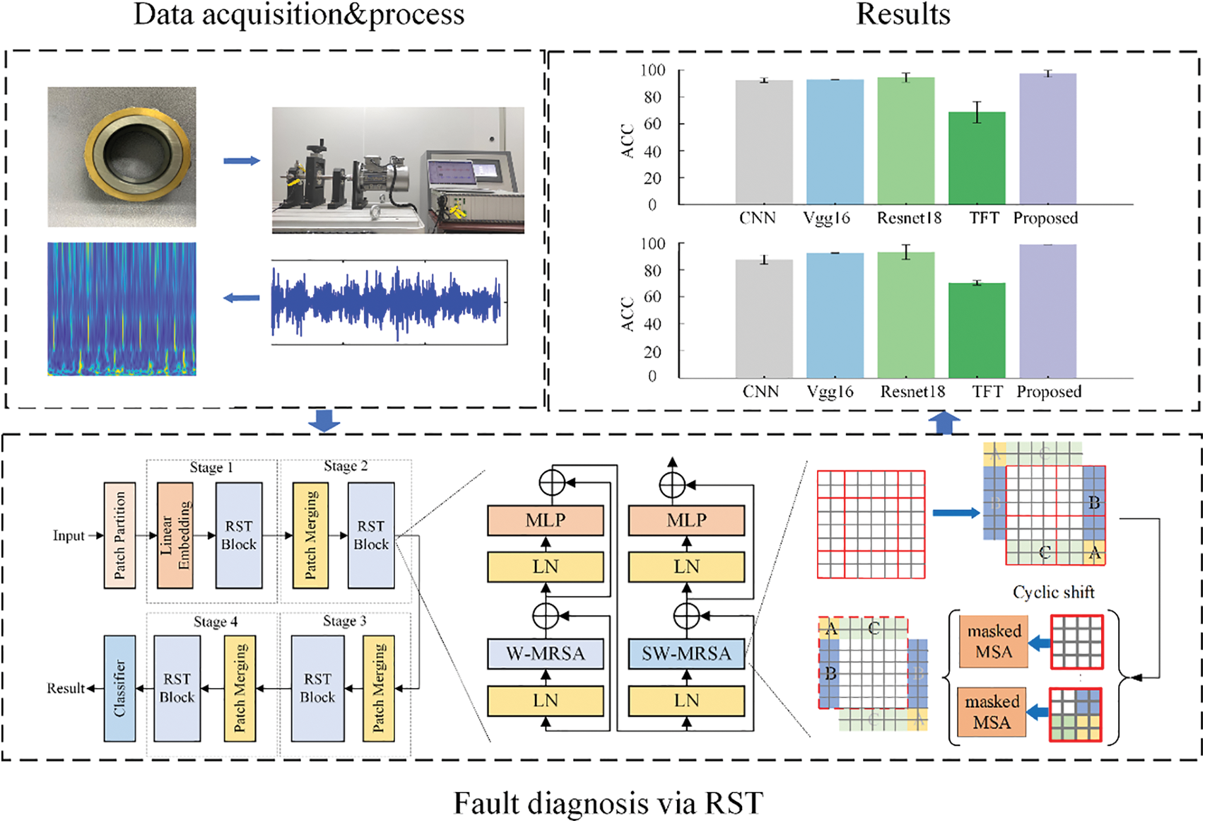
Figure 6: The implementation steps of the proposed method

Step 1: Collect 1-D vibration signals of rolling bearings under different health states;

Step 2: Convert 1-D vibrational signals into the wavelet TFDs, which will be considered as the input to the RST model. All samples are divided into a training set and a test set. The model is trained and tested on both;

Step 3: Establish the RST model, load the pre-training network parameters, and train the model by feeding the training dataset into the model. All parameters of the designed model after sufficient training; The specific process of pre-training is as follows: first, we train the model on ImageNet and save its pre-trained network parameters; Then we load these parameters before fine-tuning on the bearing dataset, and then conduct training. Loading pre-training parameters allows the network to learn the common features of image samples before fine-tuning. This can then reduce the dependence of the network on the number of samples in the target dataset, namely the bearing dataset;

Step 4: Test the trained RST model and test trained RST model’s performance.

5  Experimental Validations

5.1 Data Acquisition and Detail

5.1.1 Public Bearing Dataset

The public bearing dataset is the Case Western Reserve University (CWRU) dataset. Fig. 7 demonstrates CWRU’s experimental platform, which includes a motor, a torque sensor/decoder, and a power test meter. This paper adopts the data of 9 fault categories and one normal state of the drive end bearing. The data is collected with a 12 k sampling frequency under three kinds of motor loads of 0–3. There are three kinds of bearing fault diameters. Details are shown in Table 1.

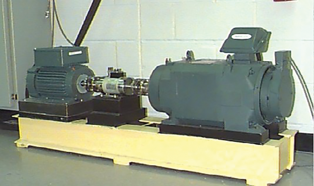
Figure 7: The rolling bearing test rig of CWRU dataset

5.1.2 Self-Built Dataset

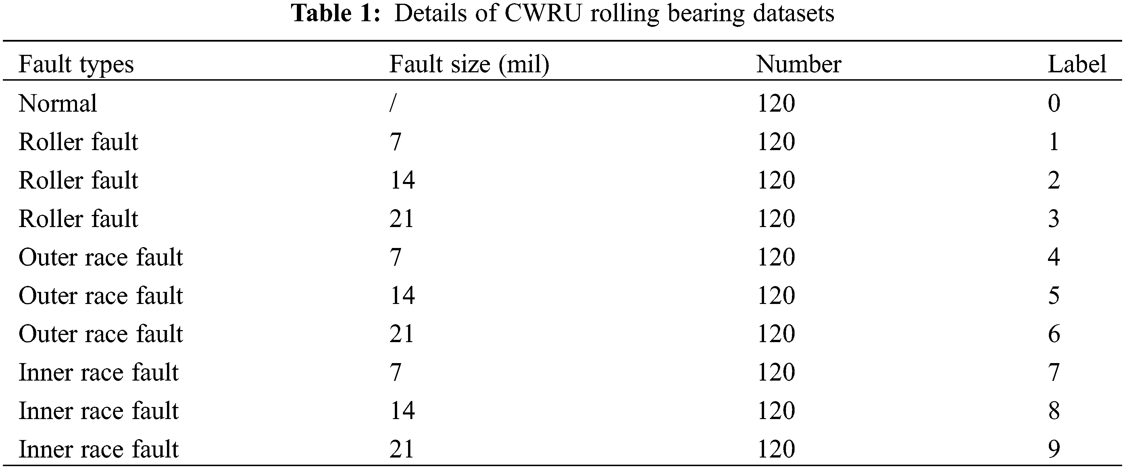
Fig. 8 shows our rolling bearing test rig, which is designed to acquire vibration signals. Three-phase asynchronous motor, motor control system, support shaft, three-support rolling bearing, and radial force loading system constitute the test rig. The test rig is equipped with three rolling bearings on a shaft, one of which is used to simulate the real fault. We refer to the self-built dataset as the Shandong University (SDU) dataset.

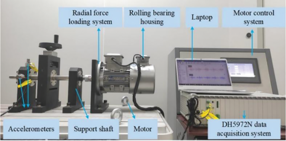
Figure 8: The rolling bearing test rig of the SDU dataset

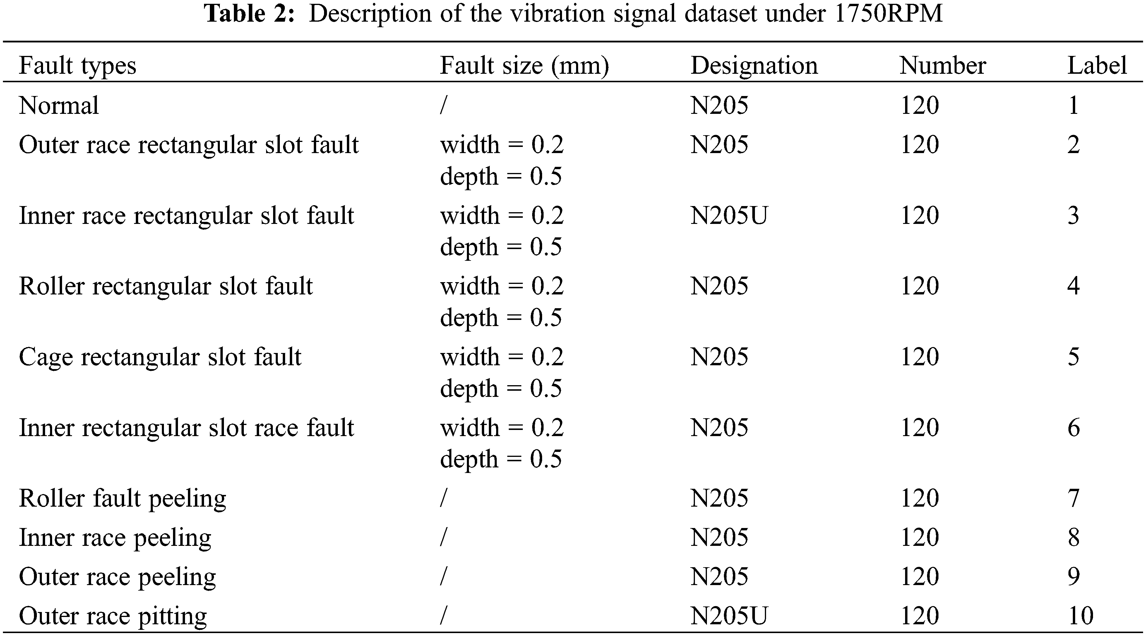
Fig. 9 displays the tested rolling bearings with different fault locations. The vibration signals under 1750RPM, whose sampling frequency is 12.8 kHz, are obtained. In our experiment, one normal state and nine fault types of data are collected. Each sample contains 4096 data points. Table 2 demonstrates the details of the SDU dataset. Rectangular slot width 0.2 mm depth 0.5 mm.

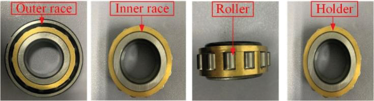
Figure 9: Tested rolling bearings with different fault locations

5.2 Case 1: CWRU Rolling Bearing Datasets

5.2.1 Experimental Setup

In this paper, MATLAB is firstly used for converting 1-D vibration signals to 2-D wavelet TFDs. The RST model is programmed in Python 3.9 with Pytorch 1.10 and runs on the Win10 operating system with Intel Xeon (R) e5-2650 V4 CPU and NVIDIA Tesla V100 GPU. Fig. 10 shows the time-domain waveforms of the CWRU dataset. The training set accounts for 90% of the total samples, and the test set accounts for 10% of the total samples. To eliminate the effects of randomness and verify our method’s the generalization capacity, we repeated ten times and took the average.

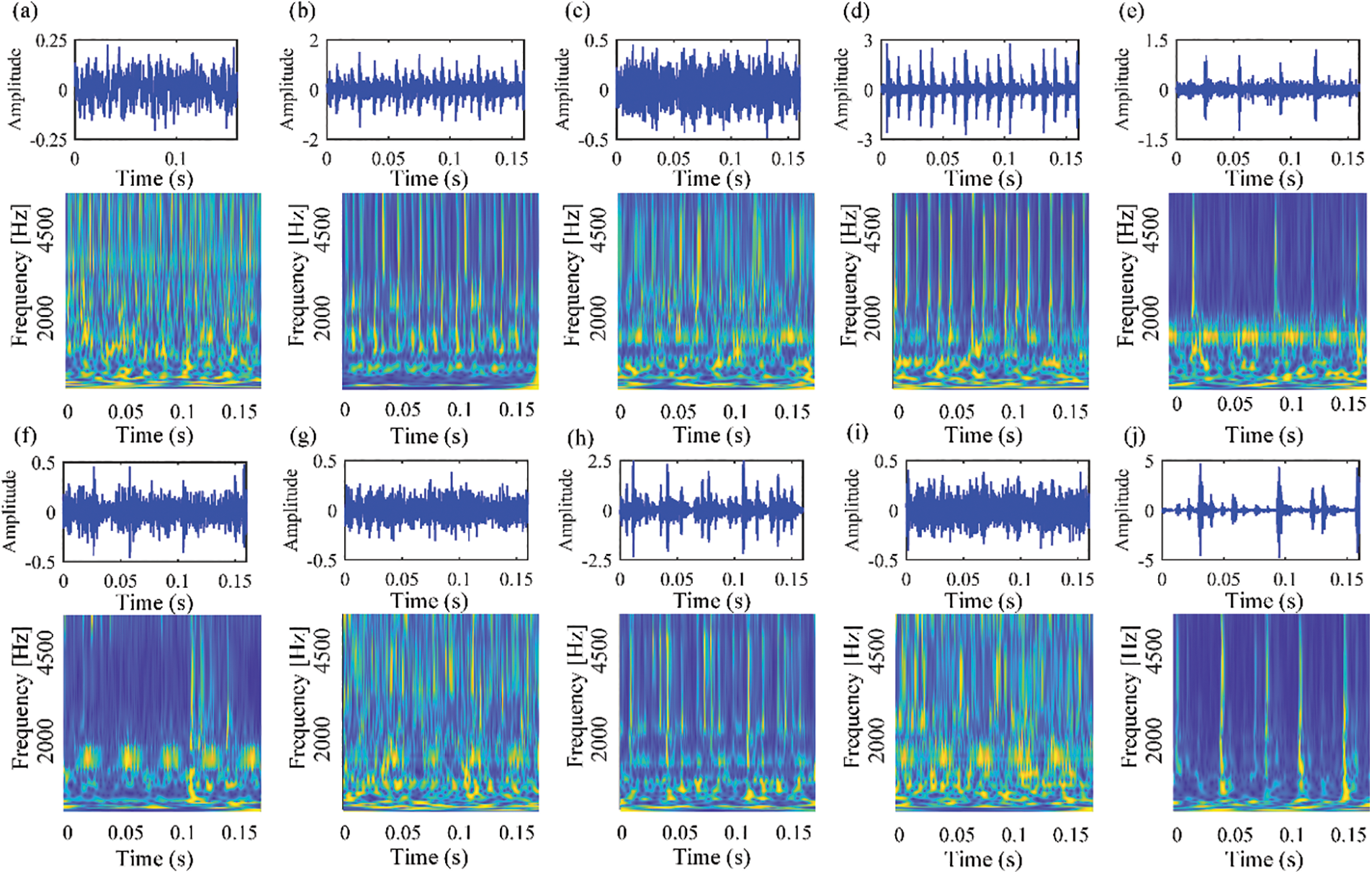
Figure 10: The time-domain waveforms and corresponding TFDs of vibration signals collected from CWRU dataset

5.2.2 Results and Discussion

We evaluate the capability of our method using the Accuracy (ACC) metric. Eq. (13) shows how it is calculated. ACC is the proportion of correctly predicted samples to the total samples. The ACC value is directly proportional to the recognition performance of the model.

ACC=1−FP+FNTP+FP+TN+FN (13)

where TP is true positives, FN is false negatives, FP is false positives, TN is true negative.

To study the effect of different parameters on the performance of the model, the RST-B model and the RST-L models were implemented for comparison. Table 3 shows the detailed structure settings of the RST-B and RST-L models. Table 4 shows hyperparameters of RST. Fig. 11 shows the training accuracy and loss curve of the RST-B and RST-L. Fig. 12 shows the RST-B and RST-L’s confusion matrix. The samples of ten categories are correctly classified. To visualize the features learned by our method, t-Distributed Stochastic Neighbor Embedding (t-SNE) lessens the high-dimensional features of the last hidden layer to 2D distribution. Fig. 13 demonstrates the 2D visualization result of features of the RST-B and RST-L. Our method divides samples of ten different labels into ten clusters, and each cluster does not contain samples of other label. Both RST-B and RST-L have good performance on the CWRU dataset. However, its training time is not as short as that of RST-B. The running times of one epoch for RST-L and RST-B are 231 and 229 s, respectively.

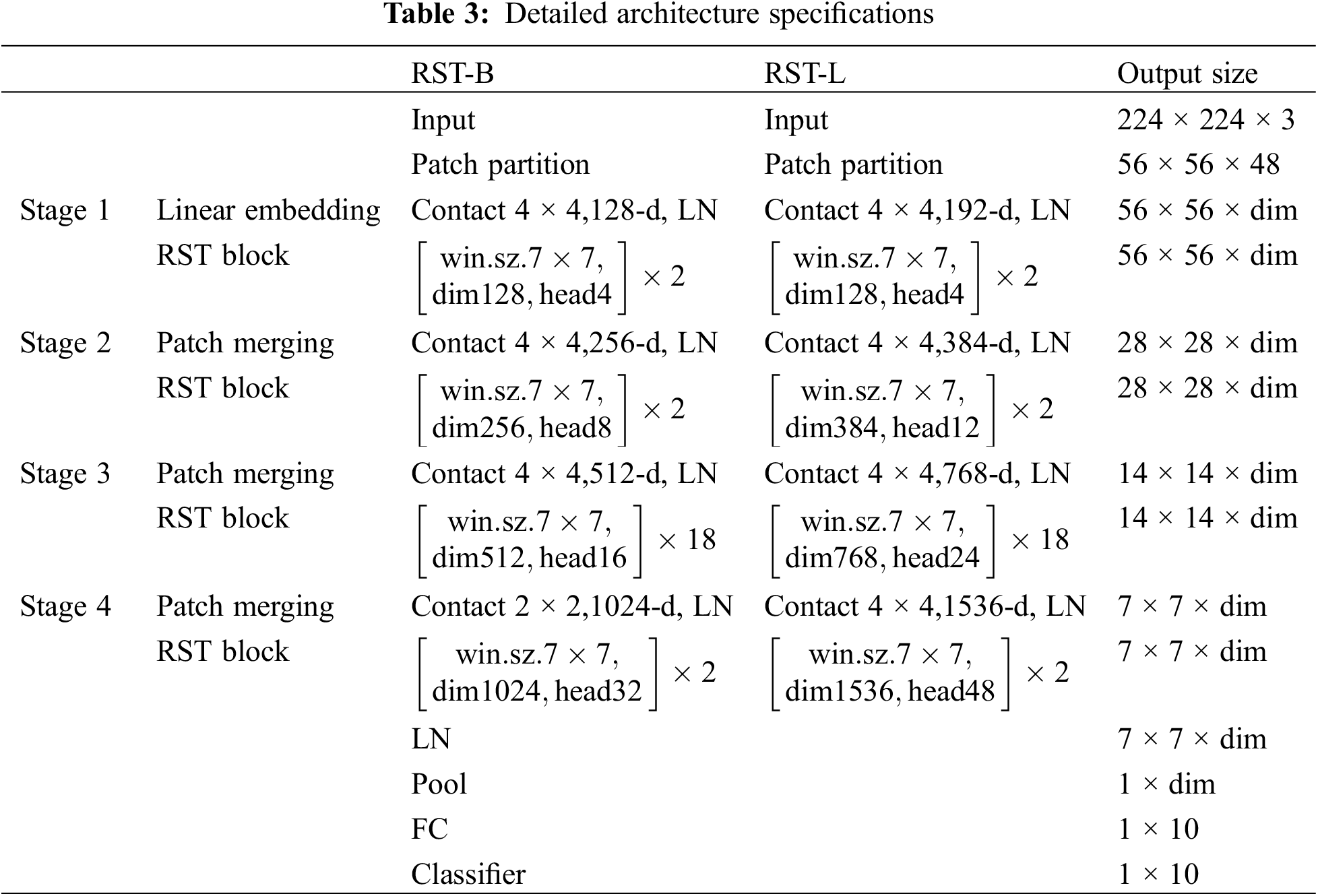
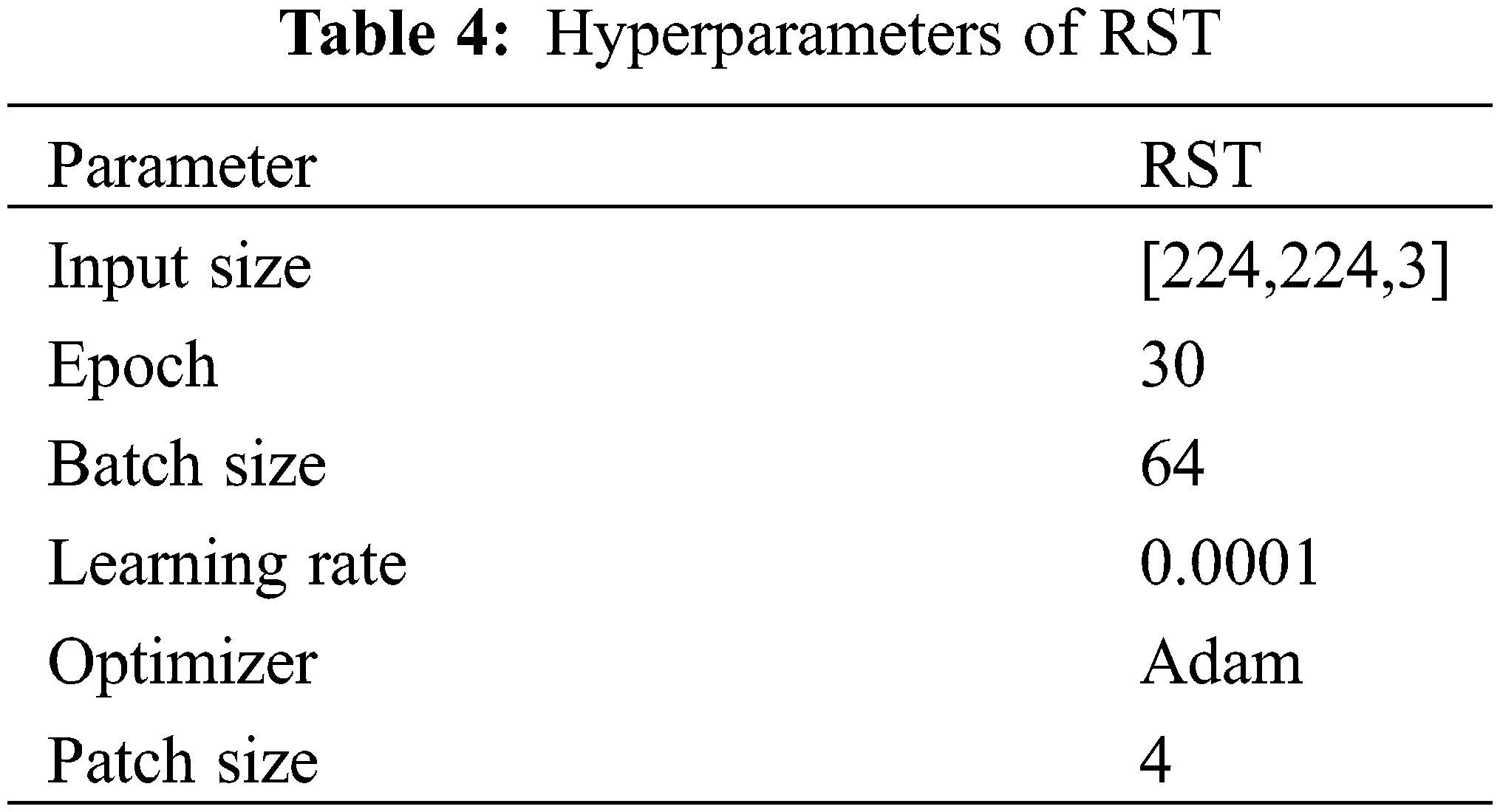
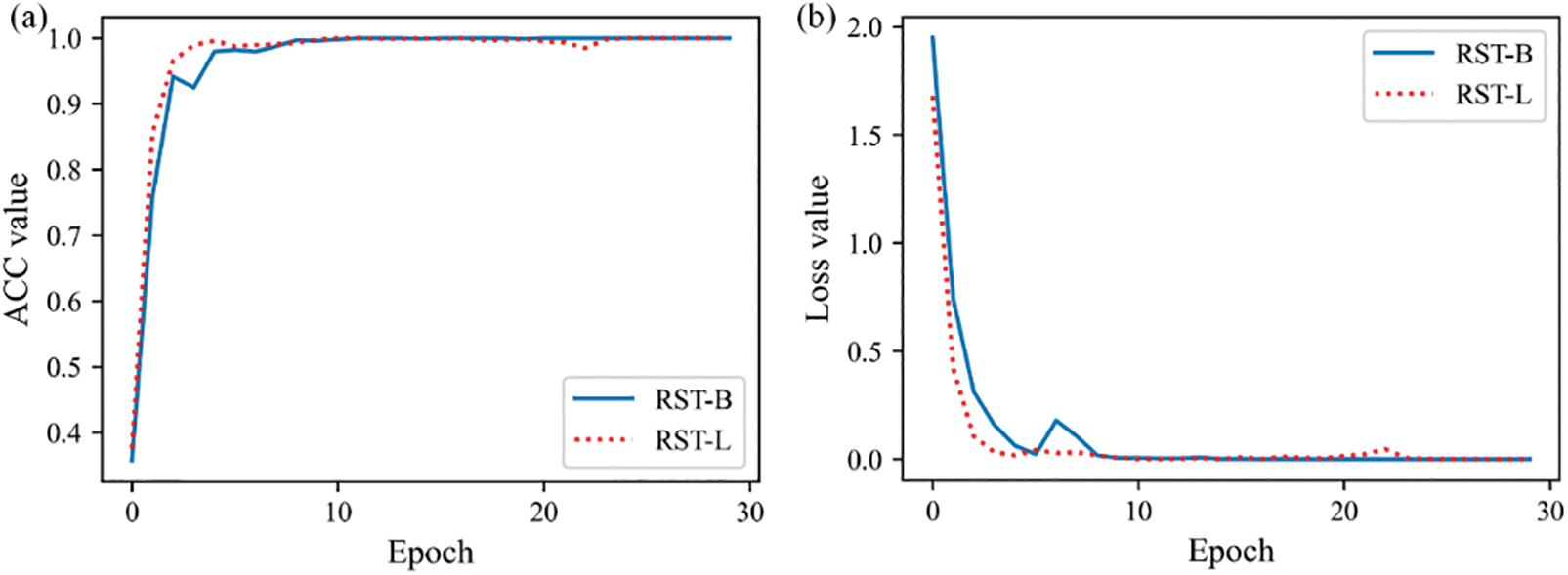
Figure 11: Results of RST model: (a) accuracy of RST and (b) loss of RST

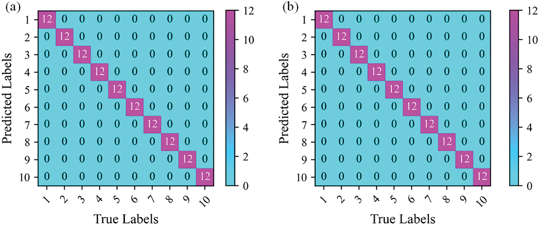
Figure 12: Confusion matrix of the proposed method for CWRU dataset: (a) RST-B and (b) RST-L

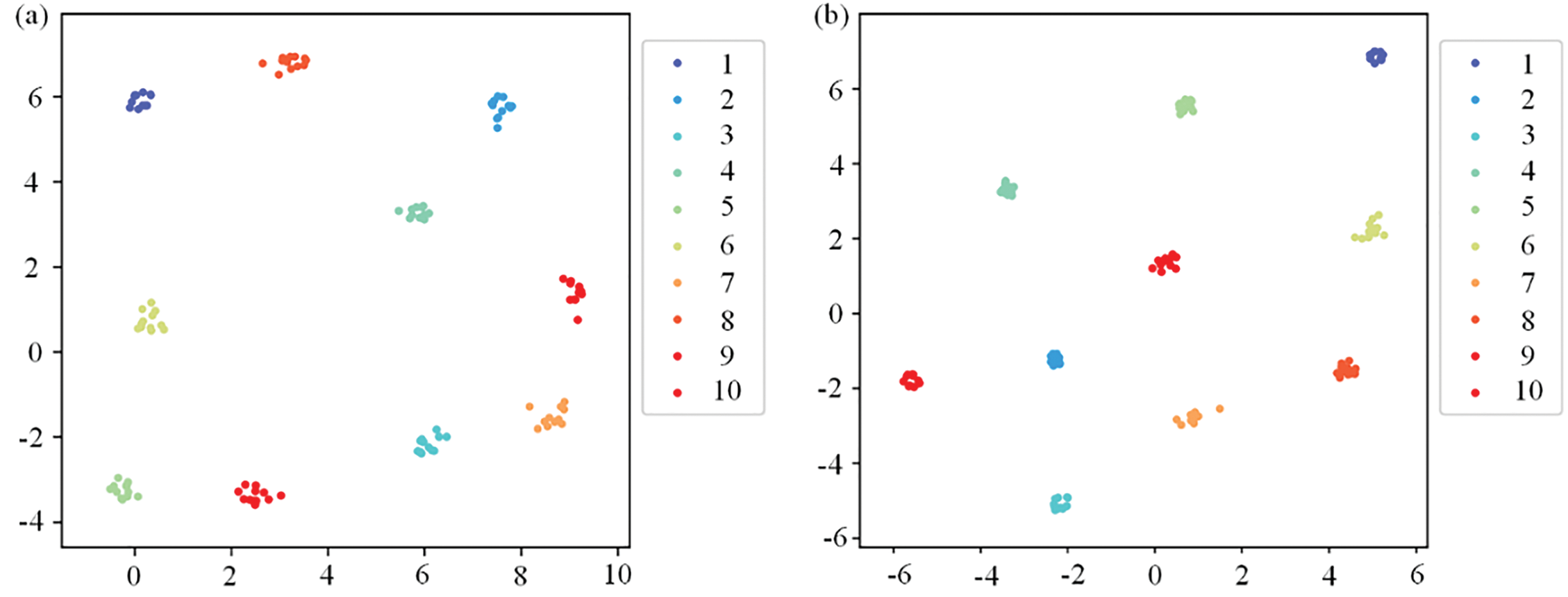
Figure 13: The 2D visualization result of features of proposed method for CWRU dataset: (a) RST-B and (b) RST-L

Our method is compared with the following methods: CNN [39], Vgg16, Resnet18, and time-frequency transformer (TFT) [40]. The parameter settings of TR-LDA, WPE+CNN, and TFT are presented in the original reference. The hyperparameter settings of TFT are the same as our method. Table 5 shows the experimental results. Our method’ ACC of under different loads are 100%, 99.81%, 100%, and 100%, respectively, which is superior to all compared methods. Fig. 14 shows our method’s performance when the training set contains different numbers of samples. Our method has a satisfactory appearance under a different number of training set samples.

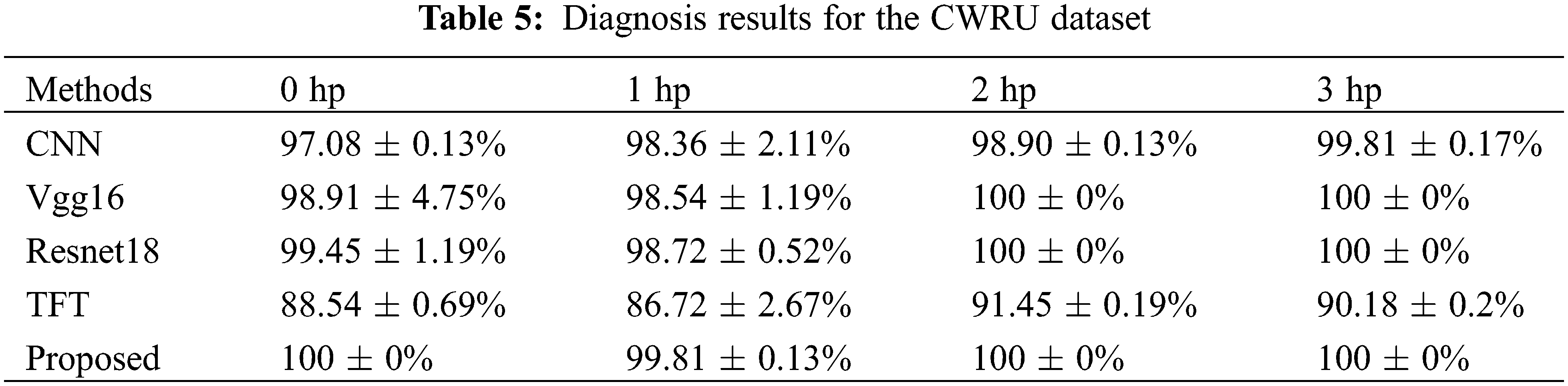
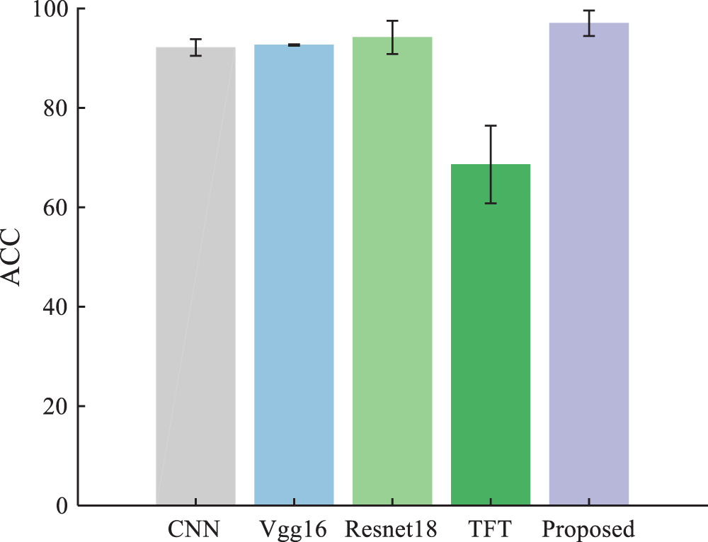
Figure 14: Experimental results of the CWRU dataset at a 3:7 ratio

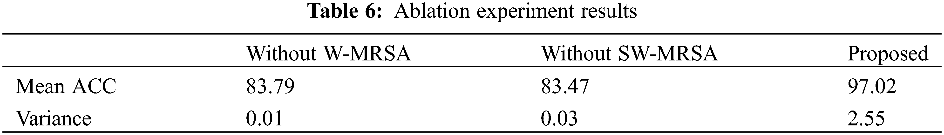
Ablation experiments were constructed to verify the effectiveness of each module in RST. The ablation experiment was selected on the CWRU dataset, with a ratio of 3:7 between training and testing. The experimental results are shown in Table 6. It can be seen that the diagnostic results of the methods without W-MRSA and SW-MRSA are lower than those of the proposed methods.

5.3 Case 2: Self-Built Dataset

5.3.1 Experimental Setup

We conducted experiments on SDU dataset to further test our method. Fig. 15 shows the time-domain waveforms of the SDU dataset. The settings of this experiment are consistent with the settings on the public dataset. The training set and test set were randomly divided from the SDU dataset, with coming from the N205 bearing.

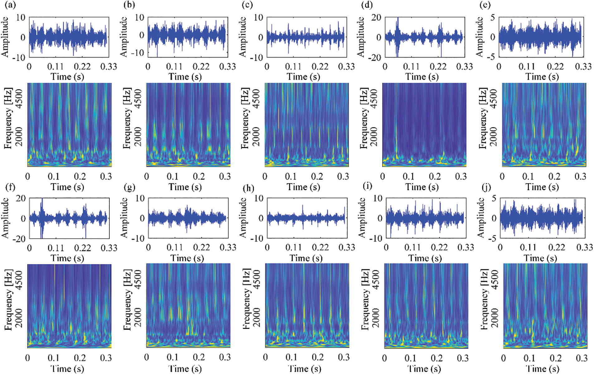
Figure 15: The time-domain waveforms and corresponding TFDs of vibration signals collected from our own rolling bearing test rig under the speed of 1750RPM

5.3.2 Results and Discussion

The hyperparameter settings of the CNN are the same as the proposed method. Table 7 shows the comparison results. Fig. 16 shows the confusion matrix of SVM, CNN, TFT, and the proposed method in the SDU dataset. Fig. 17 shows the 2D visualization result in the SDU dataset. The hidden features extracted by our method have good distinguishing ability. Fig. 18 shows the results of each method for the training and testing sets in a 3:7 partition ratio, and our method is still superior to the comparison method. Furthermore, the results demonstrate that our method can also achieve high diagnostic accuracy on different datasets.

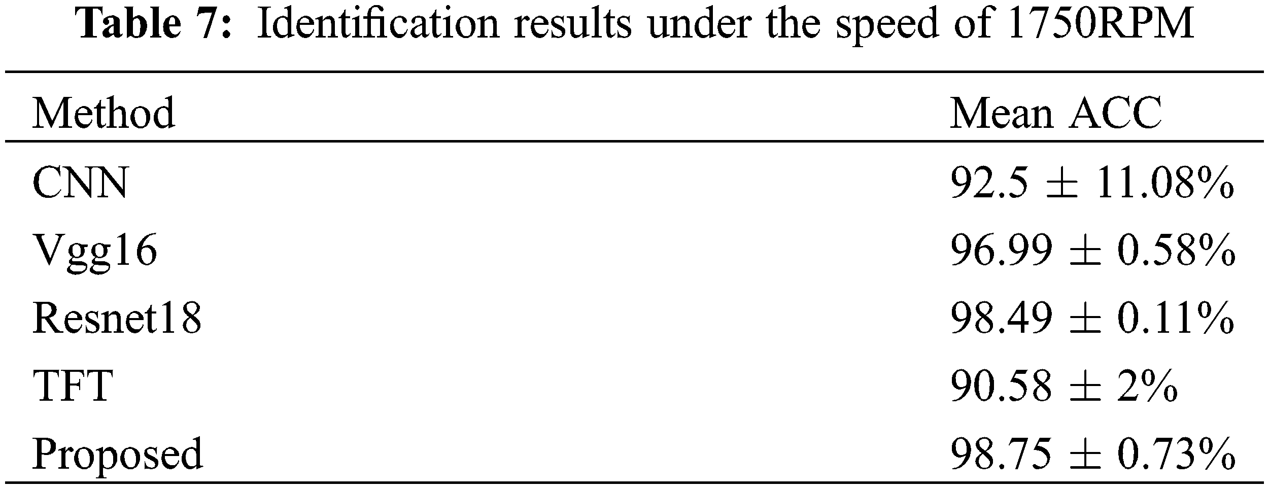
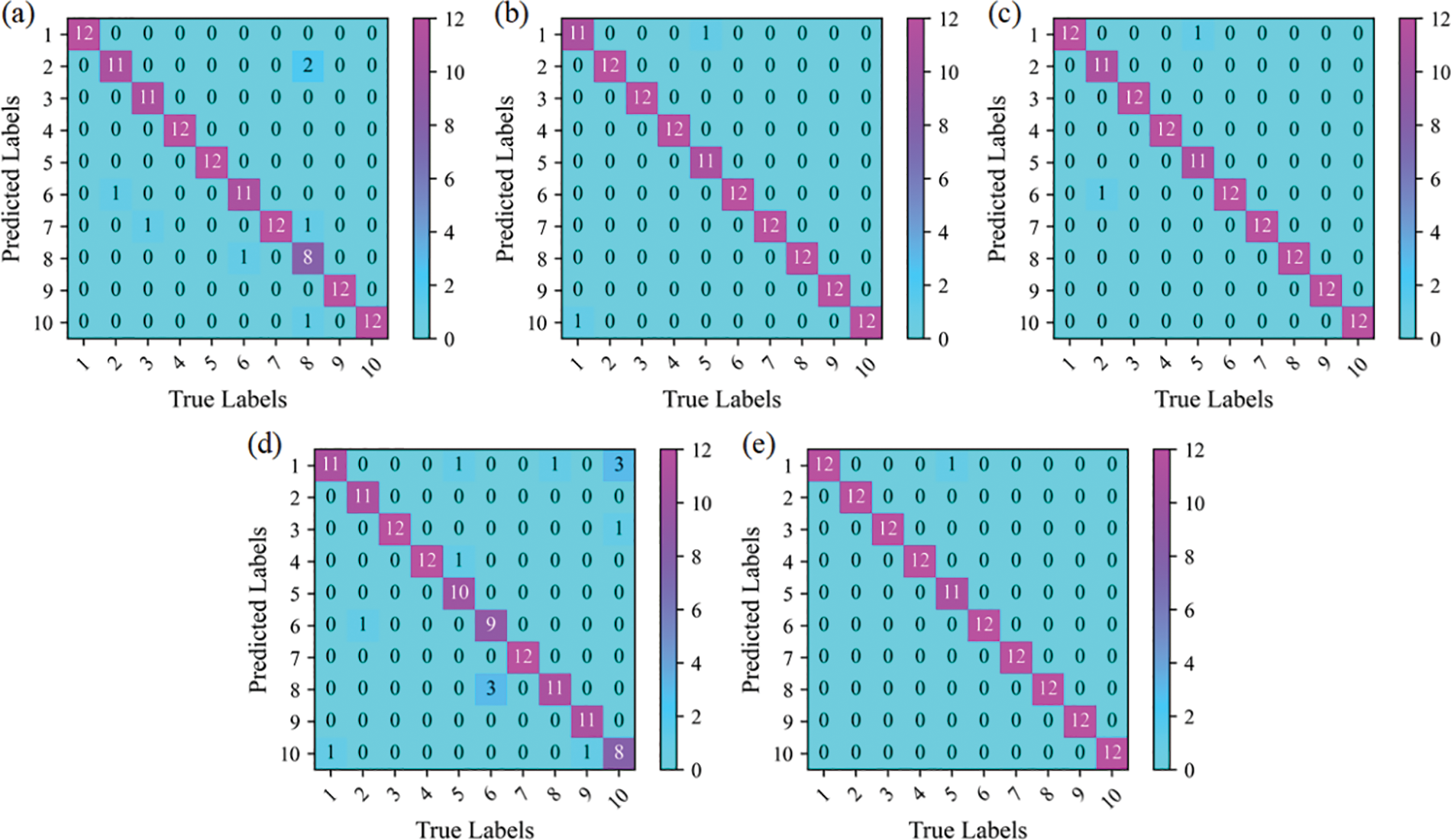
Figure 16: Confusion matrix for SDU dataset. (a) CNN, (b) Resnet18, (c) Vgg16, (d) TFT and (e) the proposed method

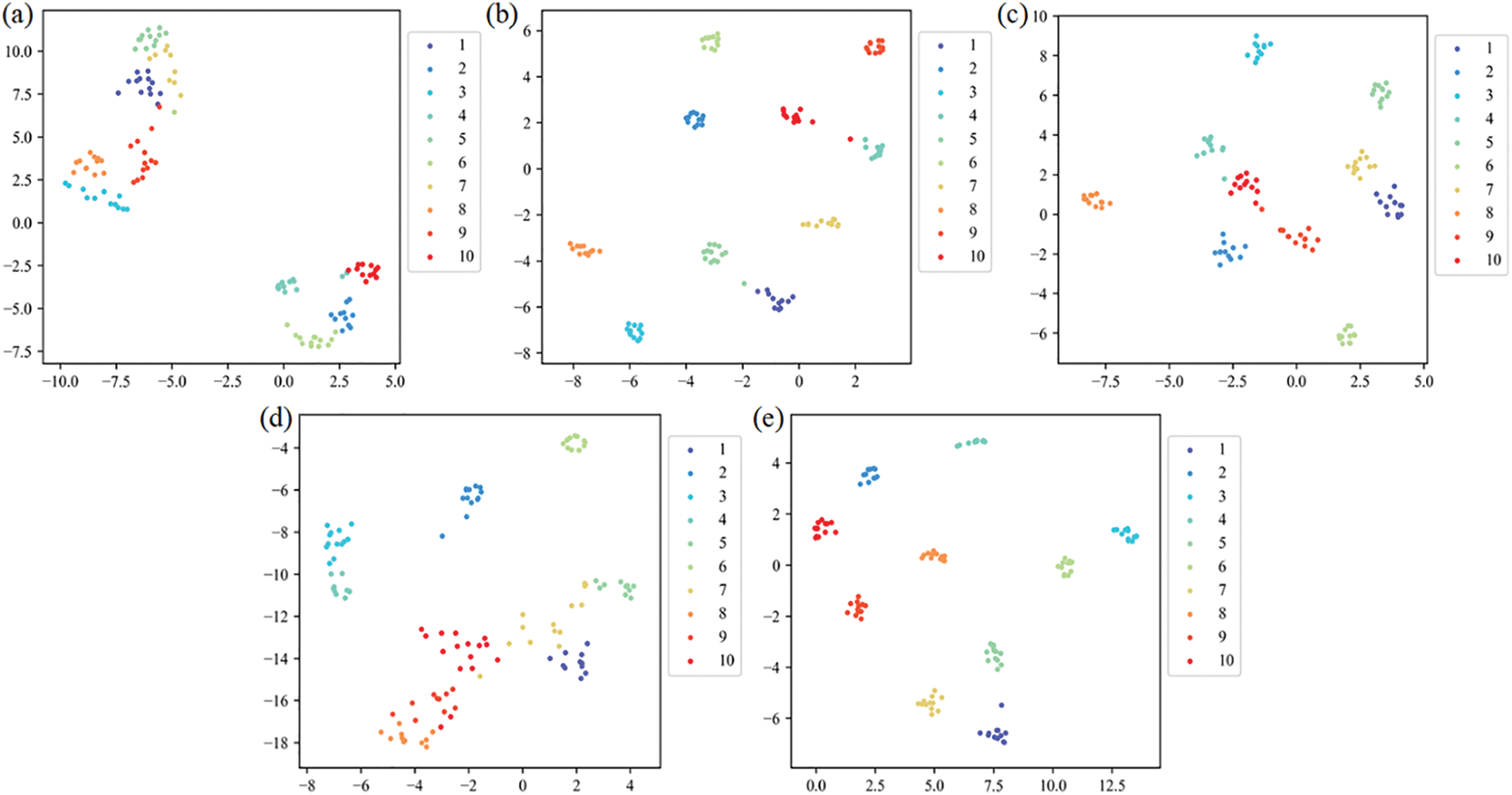
Figure 17: The 2D visualization result of features for the SDU dataset. (a) CNN, (b) Resnet18, (c) Vgg16, (d) TFT and (e) the proposed method

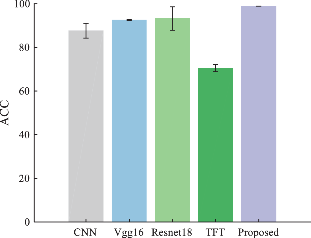
Figure 18: Experimental results of the SDU dataset at a 3:7 ratio

6  Conclusion

In this study, a novel end-to-end bearing fault diagnosis method based on transfer RST is proposed. The conclusions of this paper are as follows:

(1) Combined with TL, a novel transfer RST structure whose depth is 24 layers is created. Compared with shallow network and untrained deep network methods, the proposed method still exhibits good diagnostic performance even with limited sample data. Even with a small amount of labeled fault data, the pre-trained deep network still has good fault feature extraction ability.

(2) Our method converts the original signal into a wavelet TFD, and then inputs it into the transfer RST to obtain the fault features, and outputs the fault type.

(3) Experiments on public and SDU datasets validate our method’s performance. Under some working conditions, our method’s diagnostic accuracy is 100%. Experimental results show that our method has advantages over shallow neural networks and untrained deep neural network methods.

In the future, the proposed method will be studied in the task of classifying different mechanical equipment failure types in noisy environments.

Acknowledgement: None.

Funding Statement: This work was supported in part by the National Natural Science Foundation of China (General Program) under Grants 62073193 and 61873333 and in part by the National Key Research and Development Project (General Program) under Grant 2020YFE0204900 and in part by the Key Research and Development Plan of Shandong Province (General Program) under Grant 2021CXGC010204.

Author Contributions: The authors confirm contribution to the paper as follows: study conception and design: Haomiao Wang, Qingmei Sui; data collection: Jinxi Wang; analysis and interpretation of results: Haomiao Wang, Faye Zhang, Mingshun Jiang, Yibin Li; draft manuscript preparation: Haomiao Wang, Phanasindh Paitekul. All authors reviewed the results and approved the final version of the manuscript.

Availability of Data and Materials: The authors confirm that the data supporting the findings of this study are available within the article.

Conflicts of Interest: The authors declare that they have no conflicts of interest to report regarding the present study.

References

1. Wang, J., Zhang, Y., Zhang, F., Li, W., Lv, S. et al. (2021). Accuracy-improved bearing fault diagnosis method based on AVMD theory and AWPSO-ELM model. Measurement, 181, 109666. [Google Scholar]

2. Yan, X., Jia, M. (2018). A novel optimized SVM classification algorithm with multi-domain feature and its application to fault diagnosis of rolling bearing. Neurocomputing, 313, 47–64. [Google Scholar]

3. Luo, M., Li, C., Zhang, X., Li, R., An, X. (2016). Compound feature selection and parameter optimization of ELM for fault diagnosis of rolling element bearings. ISA Transactions, 65, 556–566. [Google Scholar] [PubMed]

4. Li, C., Sanchez, R. V., Zurita, G., Cerrada, M., Cabrera, D. et al. (2016). Gearbox fault diagnosis based on deep random forest fusion of acoustic and vibratory signals. Mechanical Systems and Signal Processing, 76, 283–293. [Google Scholar]

5. Gao, Z., Cecati, C., Ding, S. X. (2015). A survey of fault diagnosis and fault-tolerant techniques—Part I: Fault diagnosis with model-based and signal-based approaches. IEEE Transactions on Industrial Electronics, 62(6), 3757–3767. [Google Scholar]

6. Wang, D., Peter, W. T. (2015). Prognostics of slurry pumps based on a moving-average wear degradation index and a general sequential Monte Carlo method. Mechanical Systems and Signal Processing, 56, 213–229. [Google Scholar]

7. Gandomi, A., Haider, M. (2015). Beyond the hype: Big data concepts, methods, and analytics. International Journal of Information Management, 35(2), 137–144. [Google Scholar]

8. Kang, M., Islam, M. R., Kim, J., Kim, J. M., Pecht, M. (2016). A hybrid feature selection scheme for reducing diagnostic performance deterioration caused by outliers in data-driven diagnostics. IEEE Transactions on Industrial Electronics, 63(5), 3299–3310. [Google Scholar]

9. Liu, R., Meng, G., Yang, B., Sun, C., Chen, X. (2016). Dislocated time series convolutional neural architecture: An intelligent fault diagnosis approach for electric machine. IEEE Transactions on Industrial Informatics, 13(3), 1310–1320. [Google Scholar]

10. Soualhi, A., Clerc, G., Razik, H. (2012). Detection and diagnosis of faults in induction motor using an improved artificial ant clustering technique. IEEE Transactions on Industrial Electronics, 60(9), 4053–4062. [Google Scholar]

11. Prieto, M. D., Cirrincione, G., Espinosa, A. G., Ortega, J. A., Henao, H. (2012). Bearing fault detection by a novel condition-monitoring scheme based on statistical-time features and neural networks. IEEE Transactions on Industrial Electronics, 60(8), 3398–3407. [Google Scholar]

12. Boukra, T., Lebaroud, A., Clerc, G. (2012). Statistical and neural-network approaches for the classification of induction machine faults using the ambiguity plane representation. IEEE Transactions on Industrial Electronics, 60(9), 4034–4042. [Google Scholar]

13. Soualhi, A., Medjaher, K., Zerhouni, N. (2014). Bearing health monitoring based on Hilbert-Huang transform, support vector machine, and regression. IEEE Transactions on Instrumentation and Measurement, 64(1), 52–62. [Google Scholar]

14. Dong, S., Xu, X., Chen, R. (2016). Application of fuzzy C-means method and classification model of optimized K-nearest neighbor for fault diagnosis of bearing. Journal of the Brazilian Society of Mechanical Sciences and Engineering, 38, 2255–2263. [Google Scholar]

15. LeCun, Y., Bengio, Y., Hinton, G. (2015). Deep learning. Nature, 521(7553), 436–444. [Google Scholar] [PubMed]

16. Hinton, G. E., Salakhutdinov, R. R. (2006). Reducing the dimensionality of data with neural networks. Science, 313(5786), 504–507. [Google Scholar] [PubMed]

17. Sun, C., Ma, M., Zhao, Z., Chen, X. (2018). Sparse deep stacking network for fault diagnosis of motor. IEEE Transactions on Industrial Informatics, 14(7), 3261–3270. [Google Scholar]

18. Gan, M., Wang, C. (2016). Construction of hierarchical diagnosis network based on deep learning and its application in the fault pattern recognition of rolling element bearings. Mechanical Systems and Signal Processing, 72, 92–104. [Google Scholar]

19. Zhao, R., Wang, D., Yan, R., Mao, K., Shen, F. et al. (2017). Machine health monitoring using local feature-based gated recurrent unit networks. IEEE Transactions on Industrial Electronics, 65(2), 1539–1548. [Google Scholar]

20. Zhao, J., Yang, S., Li, Q., Liu, Y., Gu, X. et al. (2021). A new bearing fault diagnosis method based on signal-to-image mapping and convolutional neural network. Measurement, 176, 109088. [Google Scholar]

21. Shao, S., Yan, R., Lu, Y., Wang, P., Gao, R. X. (2019). DCNN-based multi-signal induction motor fault diagnosis. IEEE Transactions on Instrumentation and Measurement, 69(6), 2658–2669. [Google Scholar]

22. Wang, H., Liu, Z., Peng, D., Cheng, Z. (2022). Attention-guided joint learning CNN with noise robustness for bearing fault diagnosis and vibration signal denoising. ISA Transactions, 128, 470–484. [Google Scholar] [PubMed]

23. Shi, J., Peng, D., Peng, Z., Zhang, Z., Goebel, K. et al. (2022). Planetary gearbox fault diagnosis using bidirectional-convolutional LSTM networks. Mechanical Systems and Signal Processing, 162, 107996. [Google Scholar]

24. Liang, P., Deng, C., Wu, J., Yang, Z., Zhu, J. et al. (2019). Compound fault diagnosis of gearboxes via multi-label convolutional neural network and wavelet transform. Computers in Industry, 113, 103132. [Google Scholar]

25. Chen, R., Huang, X., Yang, L., Xu, X., Zhang, X. et al. (2019). Intelligent fault diagnosis method of planetary gearboxes based on convolution neural network and discrete wavelet transform. Computers in Industry, 106, 48–59. [Google Scholar]

26. Xu, Y., Yan, X., Feng, K., Zhang, Y., Zhao, X. et al. (2023). Global contextual multiscale fusion networks for machine health state identification under noisy and imbalanced conditions. Reliability Engineering & System Safety, 231, 108972. [Google Scholar]

27. Chang, Y., Chen, J., Chen, Q., Liu, S., Zhou, Z. (2022). CFs-focused intelligent diagnosis scheme via alternative kernels networks with soft squeeze-and-excitation attention for fast-precise fault detection under slow & sharp speed variations. Knowledge-Based Systems, 239, 108026. [Google Scholar]

28. Han, S., Shao, H., Cheng, J., Yang, X., Cai, B. (2022). Convformer-NSE: A novel end-to-end gearbox fault diagnosis framework under heavy noise using joint global and local information. IEEE/ASME Transactions on Mechatronics, 28(1), 340–349. [Google Scholar]

29. Zhao, Z., Zhang, Q., Yu, X., Sun, C., Wang, S. et al. (2021). Applications of unsupervised deep transfer learning to intelligent fault diagnosis: A survey and comparative study. IEEE Transactions on Instrumentation and Measurement, 70, 1–28. [Google Scholar]

30. Wen, L., Gao, L., Li, X. (2017). A new deep transfer learning based on sparse auto-encoder for fault diagnosis. IEEE Transactions on Systems, Man, and Cybernetics: Systems, 49(1), 136–144. [Google Scholar]

31. Shao, S., McAleer, S., Yan, R., Baldi, P. (2018). Highly accurate machine fault diagnosis using deep transfer learning. IEEE Transactions on Industrial Informatics, 15(4), 2446–2455. [Google Scholar]

32. Xu, G., Liu, M., Jiang, Z., Shen, W., Huang, C. (2019). Online fault diagnosis method based on transfer convolutional neural networks. IEEE Transactions on Instrumentation and Measurement, 69(2), 509–520. [Google Scholar]

33. Zhao, B., Zhang, X., Zhan, Z., Pang, S. (2020). Deep multi-scale convolutional transfer learning network: A novel method for intelligent fault diagnosis of rolling bearings under variable working conditions and domains. Neurocomputing, 407, 24–38. [Google Scholar]

34. Vaswani, A., Shazeer, N., Parmar, N., Uszkoreit, J., Jones, L. et al. (2017). Attention is all you need. Advances in Neural Information Processing Systems, 30, 5998–6008. [Google Scholar]

35. Dosovitskiy, A., Beyer, L., Kolesnikov, A., Weissenborn, D., Zhai, X. et al. (2020). An image is worth 16x16 words: Transformers for image recognition at scale. arXiv preprint arXiv:2010.11929. [Google Scholar]

36. Liu, Z., Lin, Y., Cao, Y., Hu, H., Wei, Y. et al. (2021). Swin transformer: Hierarchical vision transformer using shifted windows. Proceedings of the IEEE/CVF International Conference on Computer Vision, pp. 10012–10022. Montreal, Canada. [Google Scholar]

37. He, K., Zhang, X., Ren, S., Sun, J. (2016). Deep residual learning for image recognition. Proceedings of the IEEE Conference on Computer Vision and Pattern Recognition, pp. 770–778. Las Vegas, USA. [Google Scholar]

38. Ba, J. L., Kiros, J. R., Hinton, G. E. (2016). Layer normalization. arXiv preprint arXiv:1607.06450. [Google Scholar]

39. Zhao, Z., Li, T., Wu, J., Sun, C., Wang, S. et al. (2020). Deep learning algorithms for rotating machinery intelligent diagnosis: An open source benchmark study. ISA Transactions, 107, 224–255. [Google Scholar] [PubMed]

40. Ding, Y., Jia, M., Miao, Q., Cao, Y. (2022). A novel time-frequency Transformer based on self-attention mechanism and its application in fault diagnosis of rolling bearings. Mechanical Systems and Signal Processing, 168, 108616. [Google Scholar]