Rolling Bearing Fault Diagnosis Method Based on FFT-VMD Multiscale Information Fusion and SE-TCN Model

1  Introduction

The health condition of rolling bearings in mechanical equipment directly affects their ability to operate normally. However, in most industrial sites, these bearings face lengthy, continuous operations under high-temperature and high-pressure conditions, making them prone to failure. Therefore, accurately diagnosing rolling bearing problems is crucial to ensuring the reliability of manufacturing procedures [1].

Bearing health can be inferred from vibration signals. When the bearings fail, the signals will be accompanied by corresponding pulse responses [2]. Therefore, effective fault diagnosis can be achieved by analyzing these vibration signals [3]. Representative signal processing methods include short-time Fourier transform [4], wavelet transform [5], and empirical mode decomposition (EMD) [6], among others. Su et al. [7] proposed a hybrid filtering technique based on the autocorrelation enhancement algorithm and the best Morlet wavelet filter. First, the vibration signal was filtered by the band-pass filter, after which the filtered signal was subjected to the autocorrelation augmentation algorithm. Their results revealed that this method can eliminate interference vibration signals from other sources and can be a highly effective tool for diagnosing bearing faults. Zhang et al. [8] proposed a time-frequency analysis method based on CWT and multi-Q-factor Gabor wavelets to improve its ability to extract bearing fault information. They also conducted numerical simulations to verify whether the method accurately identify fault information. Sun et al. [9] used EMD and improved SDP image Chebyshev distance to achieve the fault diagnosis of bearings, verifying the robustness of the method through testing. Wu et al. [10] proposed an integrated empirical mode decomposition (EEMD) approach to address the aliasing problem in the EMD mode. Lei et al. [11] suggested an EEMD-based fault diagnosis method, confirming that the suggested method produced more accurate diagnosis results than the EMD approach. However, the calculation amount of EEMD is large. Torres et al. [12] proposed a complete empirical mode decomposition with adaptive noise (CEEMDAN) and reported that its effect is superior to that of EEMD. Zhang et al. [13] proposed a novel bearing fault diagnosis method combining CEEMDAN and improved TFP demodulation. Through experiments, they verified the high computational efficiency of the method. However, signal processing-based fault diagnosis calls for specialized knowledge. Furthermore, its feature extraction ability is not strong, thus posing certain limitations.

Deep learning technology has advanced quickly in recent years, and its potent feature extraction capabilities have led to its broader use in bearing fault diagnosis. Zhang et al. [14] presented a deep learning-based bearing fault diagnosis method called TICNN. This method used the original signal directly as the input, eliminating the pre-processing stage of the signal. The results of their experiment indicated that the proposed model showed excellent performance. Wang et al. [15] employed a deep CNN optimized by the particle swarm optimization (PSO) algorithm to diagnose faults in rolling bearings. Furthermore, Han et al. [16] suggested a model by combining CNN and support vector machine (SVM). Their outcomes demonstrated the model’s benefits, including high precision, good generalization ability, and less time requirement. Habbouche et al. [17] used VMD to pull features out of the original data and then input the processed data into 1D-CNN for fault diagnosis. Their outcomes demonstrated that the fault mode could be well identified. Recurrent neural networks (RNNs), which have been widely used to diagnose bearing faults, perform well in dealing with tasks related to time series. To achieve fault classification, Liu et al. [18] proposed a method for diagnosing bearing faults using RNN based on the denoising autoencoder of a gated cycle unit (GRU). Their trial results demonstrated the good diagnostic effect of the suggested method. Sabir et al. [19] first used WPD to extract features in the time-frequency domain from signals and then used these features and long short-term memory (LSTM) to classify bearing faults. Their method’s accuracy in classifying faults reached 96%. Similarly, Hao et al. [20] suggested an LSTM network-based end-to-end method, which would enhance the performance of fault diagnostics by connecting several sensors’ spatiotemporal properties. Some scholars have considered the physical information in bearing fault diagnosis to ensure that the results generated by a model align with physical laws. Ni et al. [21] proposed a novel physical information residual network (PIResNet) that provides a physically consistent solution for data. PIResNet has been shown to have high accuracy in all its experimental tasks.

In recent years, many academics have transformed original signals into two-dimensional (2D) images, using image manipulation technology to analyze and extract features. For instance, Zhang et al. [22] transformed 1D time-frequency signals using continuous wavelet transform (CWT) into 2D grayscale images and then sent the converted images to CNN for training. The trial outcomes demonstrated that this method performed well in variable working conditions. Zhou et al. [23] used the waveform image of screen capture as 2D image inputs of CNN for real-time fault diagnosis and produced favorable outcomes. Yan et al. [24] suggested a deep residual network and Markov transition field (MTF) based fault diagnosis model. They used MTF to perform dimensionality conversion on the original vibration signal, after which they established a neural network for fault diagnosis. Shen et al. [25] suggested a method based on the gram angle factory (GAF) and lightweight model E-ResNet13. In this method, they converted the original vibration signal into a 2D GAF image using a gram angler field that they then fed into E-ResNet13 for training.

Some existing deep learning-based diagnostic methods perform well under certain specific conditions. However, in actual working conditions, it is necessary to consider the impact of noise and load changes on the signal. For these reasons, fault diagnosis models must be robust and highly practicable. At the same time, using 2D for bearing fault diagnosis has some drawbacks. In particular, when performing dimensionality conversion of signals, the correlation of 1D data may be destroyed, resulting in the omission of some fault information [26]. Furthermore, using 2D feature maps for diagnosis usually requires large amounts of computing resources and lacks practical feasibility. Thus, the paper aimed to increase the precision and efficiency of diagnosing bearing faults in variable working conditions and strong noise using a multiscale information fusion method based on fast Fourier transform (FFT) and variational mode decomposition (VMD), as well as the SEnet (SE)-TCNnet (TCN) model for the fault diagnosis of rolling bearings. The innovations and main contributions of this article are as follows:

1. FFT is an excellent frequency domain analysis method, but it only provides spectrum information and cannot reflect the signal change with time. In this paper, combined with VMD, the IMF with multiscale time domain characteristics and the frequency domain components after FFT changes were reconstructed into multi-channel data. The new data, which served as an effective extension of the original data, more accurately expressed the signal’s time-frequency domain features.

2. This work improved the TCN model and increased the perception ability of the network by adding the attention mechanism, enabling the model to obtain the weight relationship of each information channel and more acutely capture the fault characteristics in the signals.

3. We conducted experimental verification using the Paderborn University bearing dataset (PU) and Case Western Reserve University (CWRU) bearing dataset, demonstrating the proposed method’s strong noise resistance and domain adaptation capabilities.

2  The Method Proposed in This Paper

2.1 TCN Model

Although CNN or RNN can be used for modeling time-series problems, both have the disadvantage of processing time series. In particular, CNN is not good at capturing long-term dependencies in time series, while RNN is prone to gradient vanishing or exploding problems. As a special CNN with a clever design, TCN comprises causal convolution, dilated convolution, and residual block. It uses convolution to extract features across time steps, enabling it to capture long-term dependencies while having the ability to perform high-speed calculations. Therefore, TCN is more suitable for dealing with time series problems [27].

1) Causal convolution. When dealing with time series tasks, TCN requires the value of the T-moment of the previous layer to rely only on the value of the T-moment of the next layer and the value before it. It cannot use future information. The formula is expressed as follows:

yt=∑i=0k−1ω(i)x(t−i)(1)

where k is the length of the convolution kernel, ω(i) is the weight of the convolution kernel at point i and xt−i is the input at point t−i. The key idea here is that the value of i cannot exceed t; so that the convolution kernel can only cover t and the values before it to ensure causality.

2) Dilated causal convolution. Causal convolution cannot prevent the model from capturing long-distance dependencies when processing time series data. A larger number of layers must be stacked to increase the receptive field and achieve good results, thus adding to the calculation costs. Dilated convolution was introduced to solve this problem. The method involves inserting “voids” between the convolution kernel elements to cover a larger input region without using additional parameters. Fig. 1 shows the structure of the dilative causal convolution. For the sequence x∈R, the formula for the dilated causal convolution is as follows:

yt=∑i=0k−1ω(i)x(t−di)(2)

where d is the dilation rate.

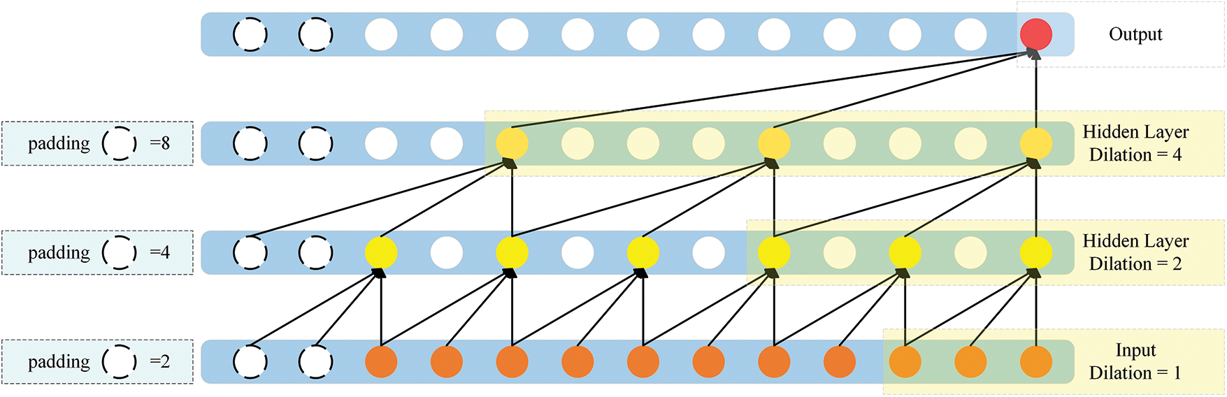
Figure 1: Structure of the dilated causal convolution

3) Residual block. Residual chaining is a useful method for deep network training because it can effectively mitigate gradient disappearance. TCN residual block contains weight normalization, ReLU activated functions, dropout layers, and dilated causal convolution. Fig. 2 presents the TCN model.

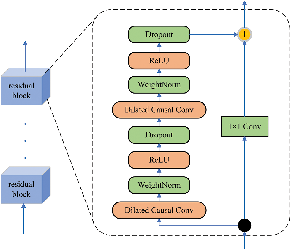
Figure 2: TCN structure

Weight normalization makes the gradient calculation more stable, thus speeding up the convergence of training. Furthermore, dropout prevents overfitting and increases robustness.

2.2 Improved TCN Model

The importance of each channel in the default input multi-channel data is equal in the dilated causal convolution. In contrast, in the actual problem, different channels have varying degrees of importance, thus limiting the network’s ability to deal with complex data relationships. This problem can be solved by embedding the channel attention in TCN. The primary function of the attention mechanism is to give greater weight to important information and less weight to unimportant information, especially when dealing with several types of information. This step ensures that the key information of the task is selected. Furthermore, embedded channel attention enables the TCN model to achieve spatial feature selection and better discover hidden temporal correlation patterns, thus improving the TCN model’s series modeling ability and generalization.

The squeeze-and-excitation (SE) network [28] is a network module proposed in 2017. The SE module obtains channel weights by explicitly modeling the interdependencies between convolutional feature channels, which reflect the degree of contribution to the task, and then reweighting the original data. Fig. 3 shows the SE network (SEnet).

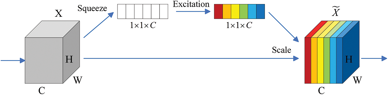
Figure 3: Structure of SEnet

SEnet consists of the Squeeze, Excitation, and Scale operations.

Squeeze operation: This step compresses the data for each input channel. Through global average pooling, the data containing global information is compressed into a feature vector of 1×1×C as follows:

Zc=Fsq(Xc)=1H×W∑i=1H∑j=1Wxc(i,j)(3)

where Zc is the output after compression, Xc is the input, and xc(i,j) is the value of the element whose coordinate is (i,j) in the c channel.

Excitation Operation: The compressed feature vector Zc passes through two FC layers. The FC layer is activated by ReLU, and the second FC layer is activated by Sigmoid. The learned channel correlation is converted into a probability value of 0∼1 expressed as:

s=Fex(Zc,W)=σ(g(Zc,W))=σ(W2δ(W1Zc))(4)

where s is the output obtained after the excitation operation, W1 is the weight matrix with dimension (c/r)×c, W2 is the weight matrix of dimension c×(c/r), r is the reduction ratio, δ is the ReLU activation function, and σ is the Sigmoid activation function.

Scale operation: In this step, the resulting weight s is multiplied with the original input X to obtain the final output X~. This is expressed as follows:

X~=Fscale(Xc,sc)=Xc⋅sc(5)

The framework of the SE network and TCN (SE-TCN) is shown in Fig. 4. The SE-TCN block embeds the SE attention in the residual block of TCN. The whole model consists of three stacked SE-TCN blocks, and the feature classification is carried out by adaptive average pooling and linear layer. Finally, the results are output.

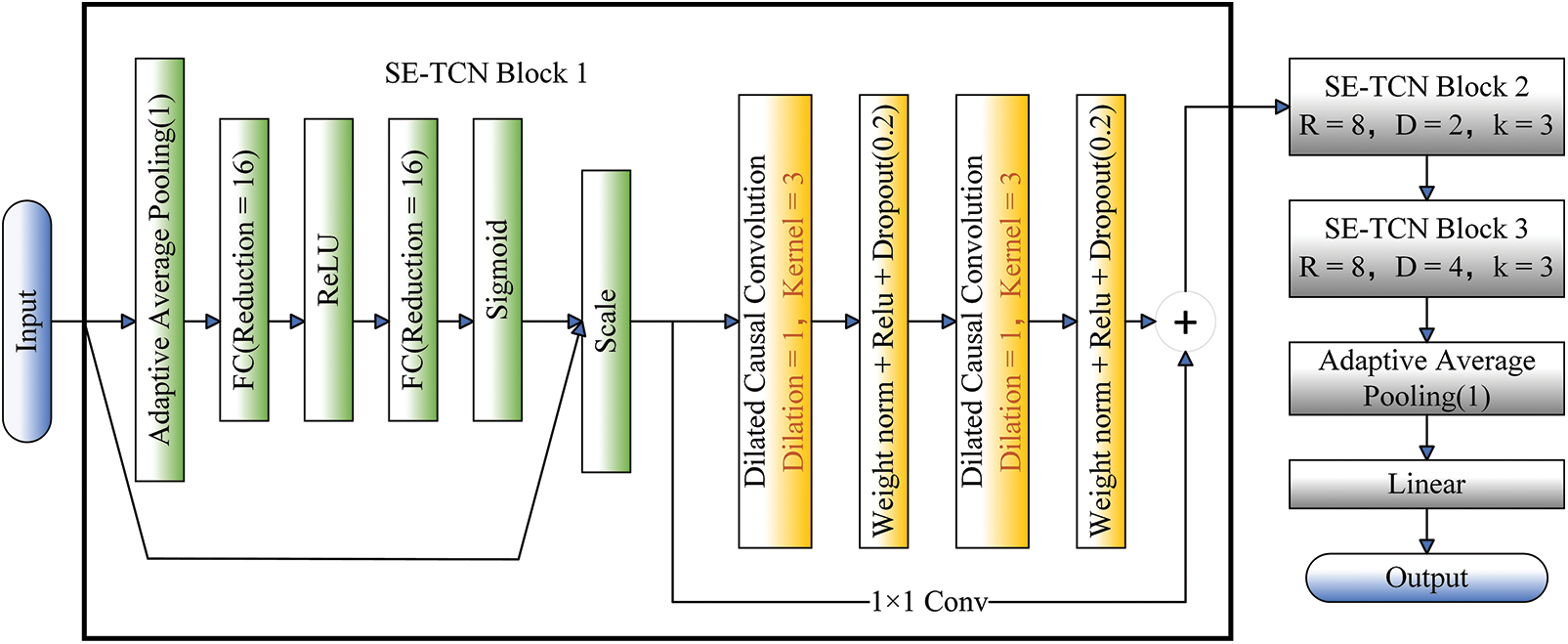
Figure 4: SE-TCN structure

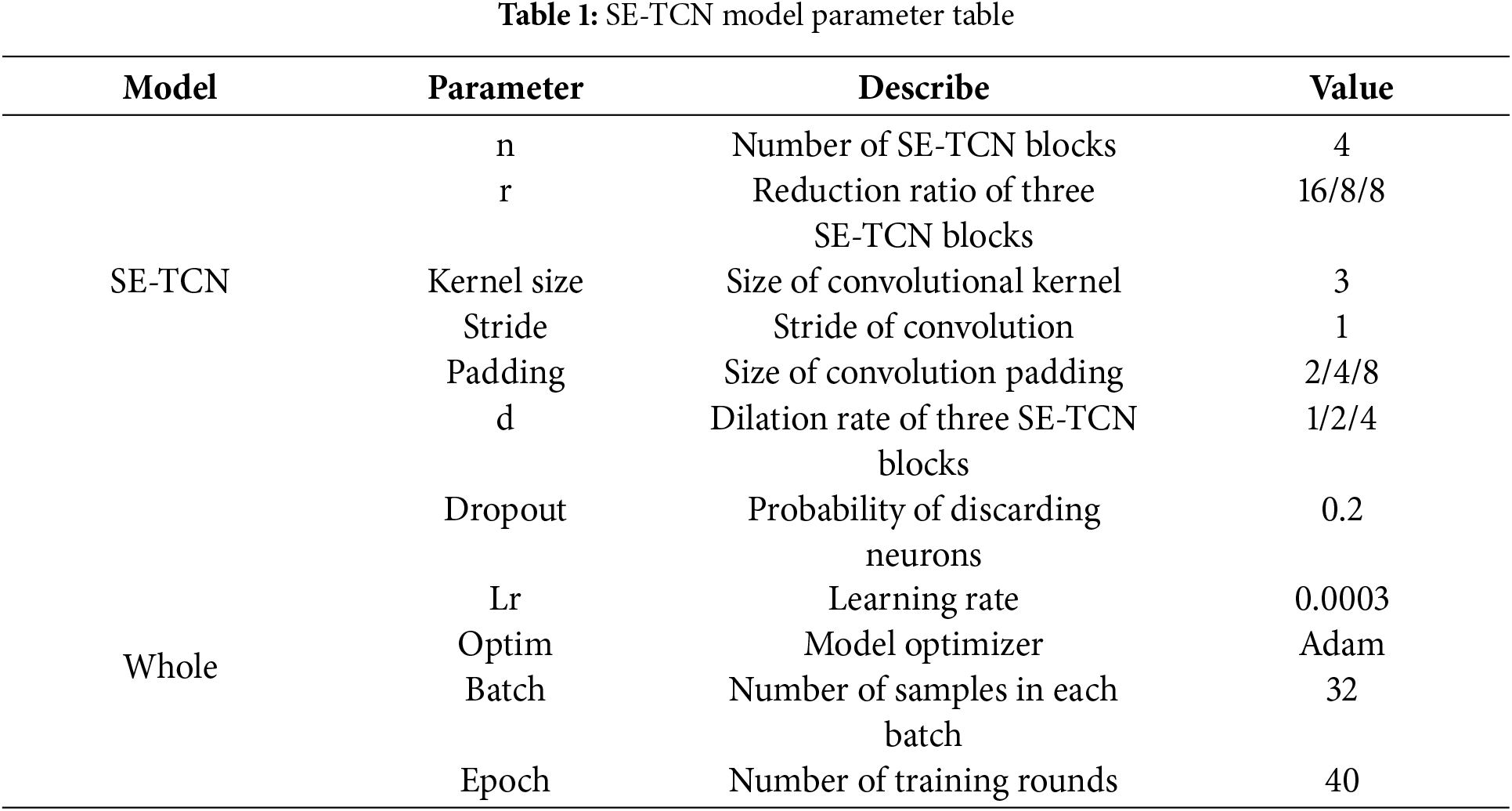
SE attention strengthens the processing of the relationship between the vibration signal channels and further highlights key information. The reduction ratio of the first SE-TCN block is 16, reducing the number of parameters while ensuring good performance. The reduction ratio of the latter two SE-TCN blocks is 8, which captures global features more comprehensively, and the TCN residual block increases the processing of context information concerning vibration signals. The three SE-TCN blocks have a convolution kernel size of 3, and the dilation rates are 1, 2, and 4. Without increasing the number of layers or kernel size to enhance parameters, this structure can rapidly increase the receptive field. Table 1 shows the model parameter values.

2.3 Data Processing

2.3.1 Data Source

The CWRU-bearing dataset used for experiments is available to the public. The experimental platform of the CWRU dataset consisted of a motor, torque sensor, coupling, and load motor. The acceleration sensor on the motor base is used to collect vibration signals from the bearings. The data used in the experiment came from the SKF6205 deep groove ball bearing at the driving end, with a sampling frequency of 12 KHZ. The fault in the dataset is the use of EDM technology to set faults for bearings. The faults are 0.007, 0.014, and 0.021 inches in size. The fault location includes the inner ring, outer ring, and rolling element, and a total of 9 types of faults were obtained. The dataset also included data under 0~3 hp working conditions. In this experiment, signals collected under three working conditions of 0~2 hp were selected.

2.3.2 Data Enhancement

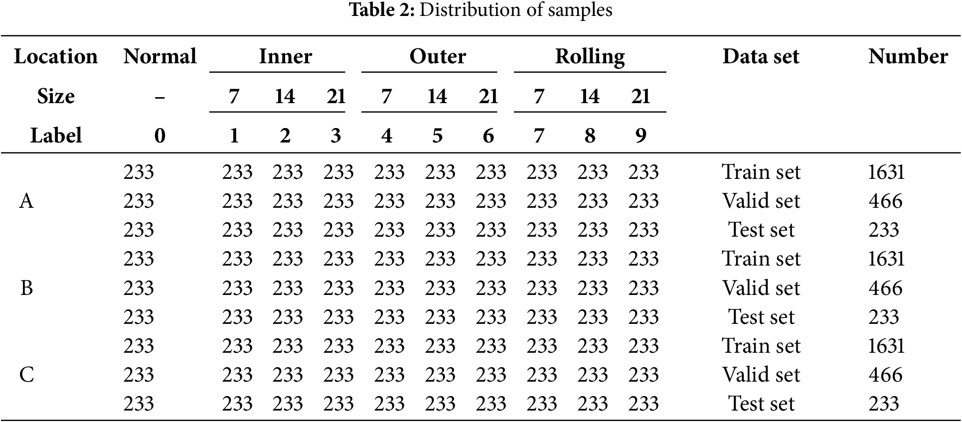
Given that the dataset had inadequate data, the sliding window overlapping sampling approach enhanced the data, effectively reducing overfitting. The sliding window and step sizes were 1024 and 512, respectively. The diagram of overlapping sampling is shown in Fig. 5. Three datasets were obtained using this sliding window to extract data for the three 0~2 hp working conditions, symbolized by A, B, and C in that order. Every load contained 2330 data samples. All three datasets contained nine types of fault and healthy samples, with a total of 10 types of sample data. The ten types of samples were labeled from 0 to 9 and divided in a ratio of 7:2:1. Table 2 shows the distribution of the sample.

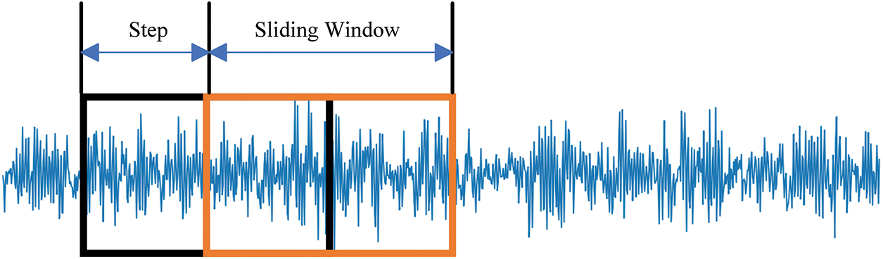
Figure 5: Overlapping sampling

2.3.3 Information Fusions

In essence, a bearing’s failure signal is a cyclic stationary signal containing a certain periodicity [29]. Bearing failure can alter the vibration signal’s specific frequency components, and in this case, FFT is an excellent method to deal with these signals. The natural and fault characteristic frequencies of bearings can be efficiently identified with FFT. These frequency components are an important basis for bearing fault diagnosis.

However, a single-frequency domain processing method cannot capture the fault characteristics comprehensively, and FFT can only provide the spectrum information of signals at a certain moment, making it unable to reflect how signals change over time. Thus, VMD is introduced to solve this issue. VMD is a non-recursive adaptive signal processing technique [30] that extracts the inherent oscillation pattern from the complicated signal, thus breaking the signal down into a series of IMFs with different central frequencies. Various components can represent time domain information in different frequency intervals.

In using VMD to decompose a vibration signal f into k finite bandwidth modes, the constraint expression is as follows:

{min{uk},{ωk}{∑k=1K‖∂t[(δ(t)+jπt)∗uk(t)]e−jωkt‖22}s.t∑k=1Kuk=f(6)

where k is the number of decomposition modes, {uk} is the k-th mode component after decomposition, {ωk} is the center frequency of the k-th mode after decomposition, δ(t) is the Dirac function, ∂(t) is the gradient operation, and ∗ is the convolution operation. Introducing the Lagrangian operator λ to obtain an augmented Lagrangian expression:

L({uk},{ωk},λ)=α∑k=1K‖∂t[(δ(t)+jπt)∗uk(t)]e−jωkt‖22+‖f(t)−∑k=1Kuk(t)‖22+⟨λ(t),f(t)−∑k=1Kuk(t)⟩(7)

where α is the penalty factor. The modal component uk and center frequency ωk are iteratively solved using the following alternating direction multiplier method:

u^kn+1(ω)=f^(ω)−∑i≠ku^i(ω)+λ^(ω)21+2α(ω−ωk)2(8)

ωkn+1=∫0∞ω|u^kn+1(ω)|2dω∫0∞|u^kn+1(ω)|2dω(9)

where ω is the frequency, and n represents the number of iterations.

Taking the first normal sample as an example, the signal was decomposed via FFT and VMD. The resulting frequency-domain signal and the IMFs stacked into a new multi-channel data (Fig. 6) are called information fusion data (IFD). These data containing multiscale time-frequency domain information can fully reflect the bearing fault characteristics. This method formed all samples from the above datasets into a new dataset.

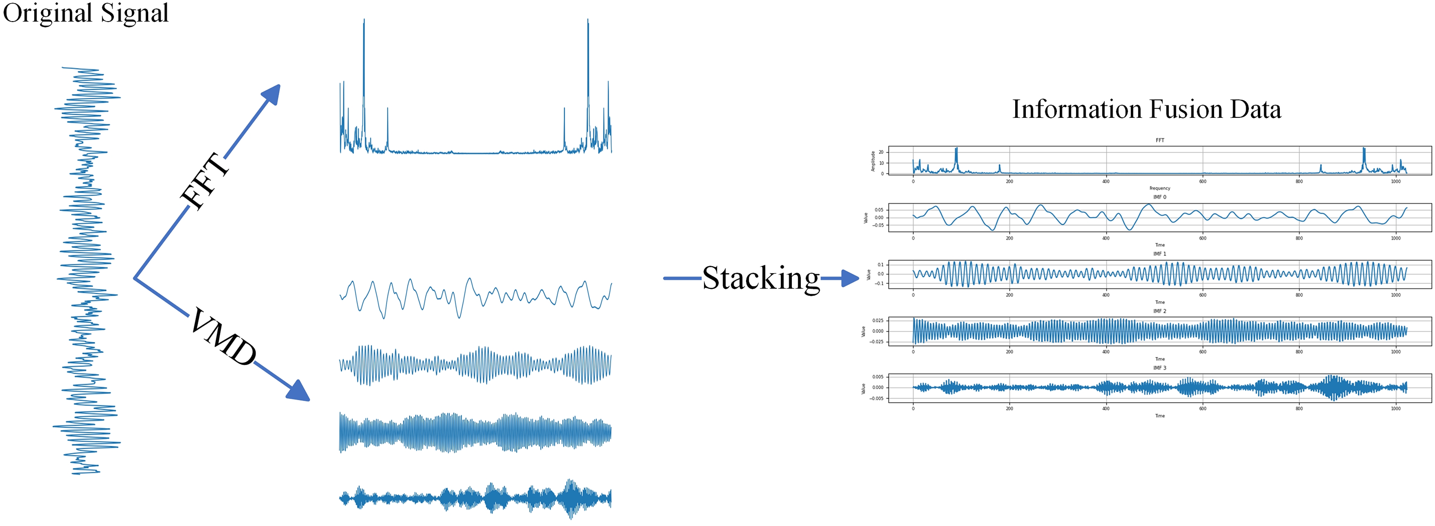
Figure 6: Information fusions of the data

In the above VMD, the number of mode decomposition k was determined using the center frequency approach. Through program decomposition, the penalty factor (alpha) in the program was set to 2000, thus avoiding the phenomenon of mode mixing. The noise tolerance (tau) was set to 0, and the initialization method (init) was set to 1. All center frequencies were initialized uniformly. The tolerance of convergence (tol) was set to 1 × 10-7. In addition, the value of k was set to 2, 3, 4, 5, 6, and 7, and the center frequencies of each modal component with different decomposition numbers were obtained. Table 3 shows the results.

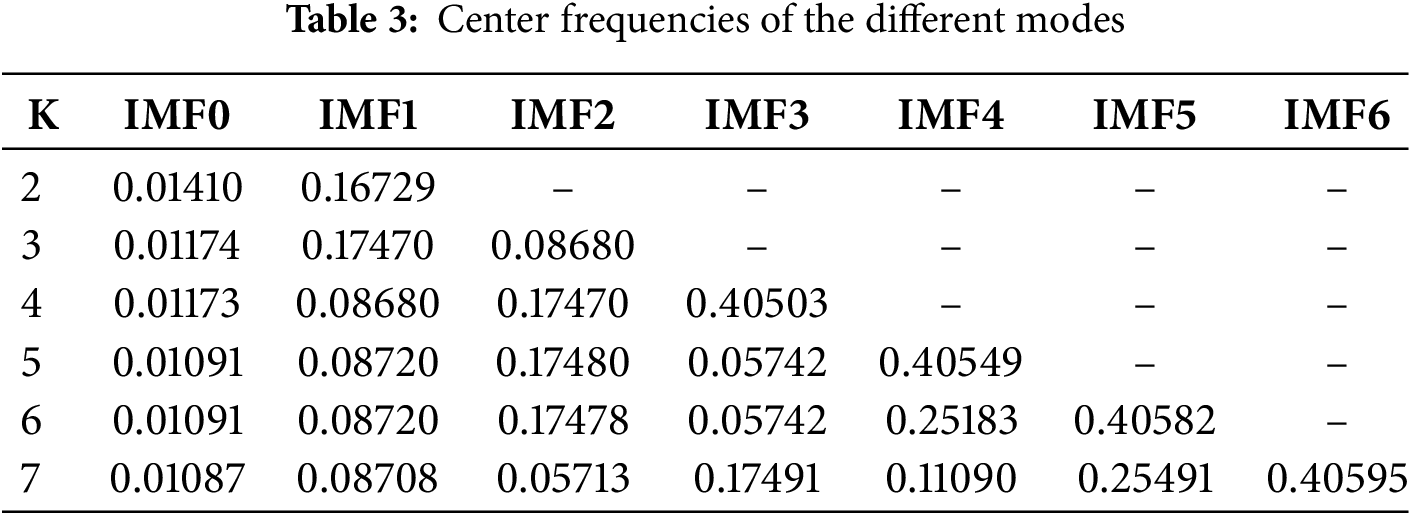
The center frequencies were observed based on different k-value conditions. From K = 4 onwards, modes with similar center frequencies appeared, indicating over-decomposition. Thus, the number of mode decomposition K was selected as 4. This choice avoids unnecessary over-decomposition, reduces computational complexity, and improves efficiency.

2.4 General Framework of the Proposed Method Suggested in This Paper

Fig. 7 shows the framework of the proposed fault diagnosis method. First, signals were captured through overlapping sampling. Then, the intercepted signal was processed by FFT and VMD, after which the newly generated data were stacked. Next, the IFD was separated into training, validation, and test sets. Finally, the generated dataset was sent to the SE-TCN model for training. The data were successfully passed through three SE-TCN blocks with different dilation rates during training. Layer by layer, the network’s receptive field increased, and the network captured features of different time scales at varying levels. The output feature matrix of the network is then passed through the Softmax to obtain the probability distribution of classification.

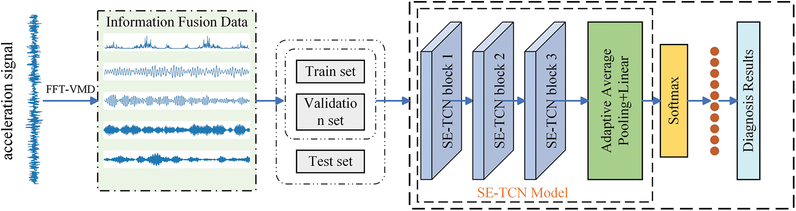
Figure 7: Overall structure of fault diagnosis method

3  Experiments and Analysis

3.1 Model Training

The Python version used in this paper is 3.8. During model training, the mini-batch value was set to 32, and the epoch value was set to 40. The training automatically stopped when the preset round was reached. The cross-entropy loss function and Adam optimization algorithm were used to update model parameters. The learning rate was set to 0.0003. Five experiments were repeated to exclude the potential impact of chance on the outcomes.

Bi-GRU, GoogLeNet, and TCN were used as contrast models to demonstrate the proposed model’s superiority. At the same time, IFD+SE-TCN, VMD+SE-TCN, and FFT+SE-TCN were used for comparative experiments to verify the effectiveness of the proposed multiscale information fusion method. Fig. 8 shows the performance of each model running once on dataset C. In contrast, Table 4 shows the accuracy of each method after training on three datasets to determine the performance differences of each method more intuitively.

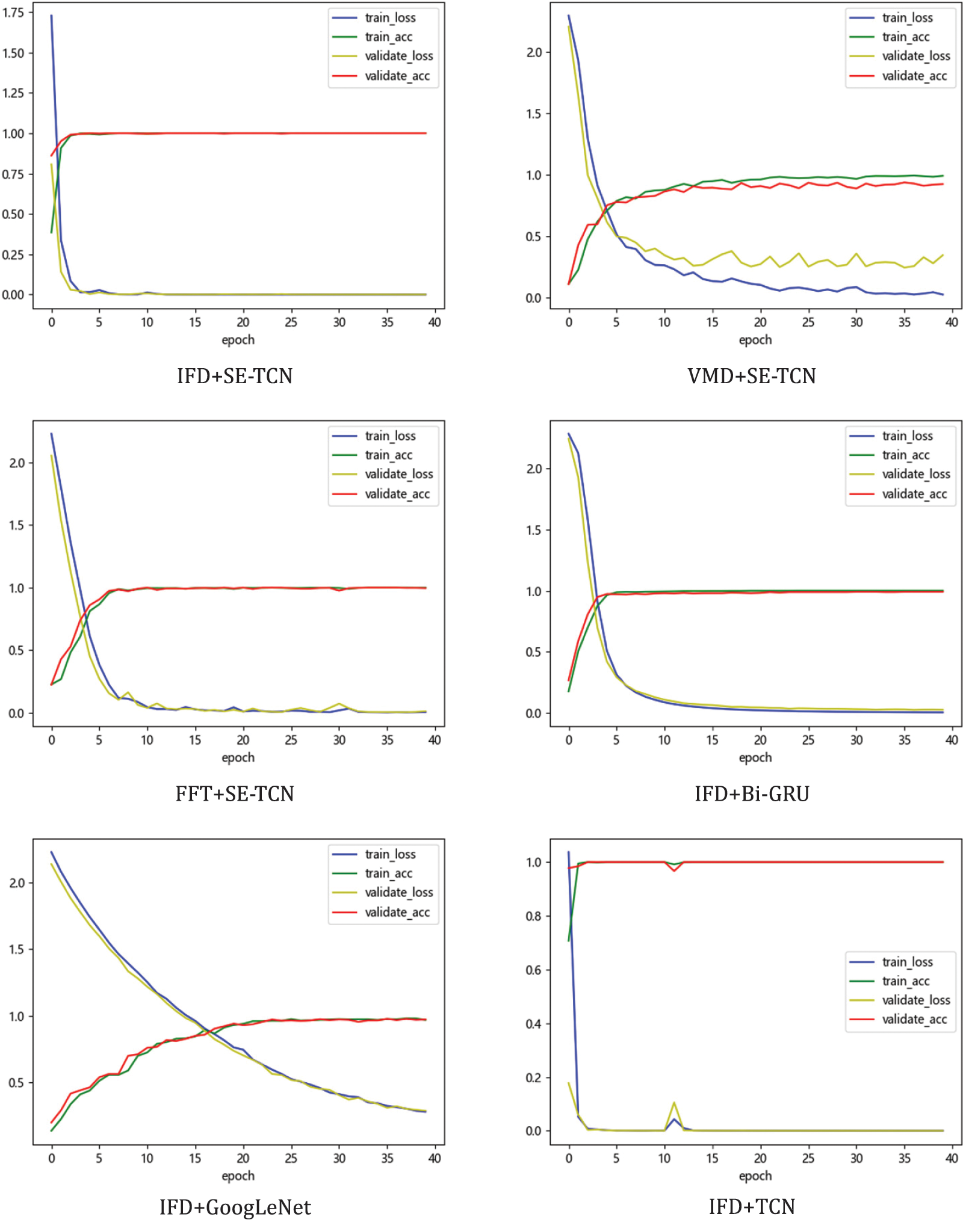
Figure 8: Training results of each method

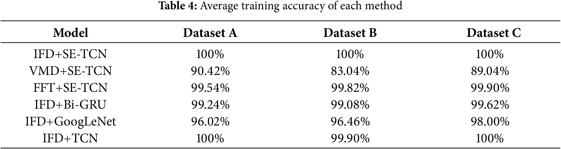
As shown in Table 4, in the model performance comparative experiment, the accuracy of SE-TCN on three datasets, A, B, and C, reached 100%, which is higher than that of Bi-GRU and GoogLeNet. These results indicate that SE-TCN can classify bearing faults accurately. The accuracy of SE-TCN is 0.1% higher than that of TCN on dataset B, demonstrating that, by introducing an attention mechanism, the model can focus more on key features when processing information fusion sequences, thus leading to improved model performance. In the comparative experiment of different pretreatment methods, the accuracy of IFD+SE-TCN is higher than that of VMD+SE-TCN and FFT+SE-TCN, indicating the superiority of the multiscale information fusion pretreatment method.

3.2 Performance Analysis under Different Noise Conditions

Table 4 shows that all methods have excellent accuracy when noise interference is absent. However, some weak fault features will be difficult to extract under actual working conditions, which are accompanied by noise. This section discusses the accuracy of the proposed method under noisy conditions. In this section, only dataset C was used for training. White noise was introduced to the vibration signal to generate signals with different SNRs. The SNR formula is expressed as follows:

SNR(dB)=10×log10⁡(PsignalPnoisc)(10)

where Psignal is the signal power, and Pnoisc is the noise power. As shown in the formula, the smaller the SNR, the greater the impact on the original signal. Fig. 9 shows the model accuracy under different SNR conditions.

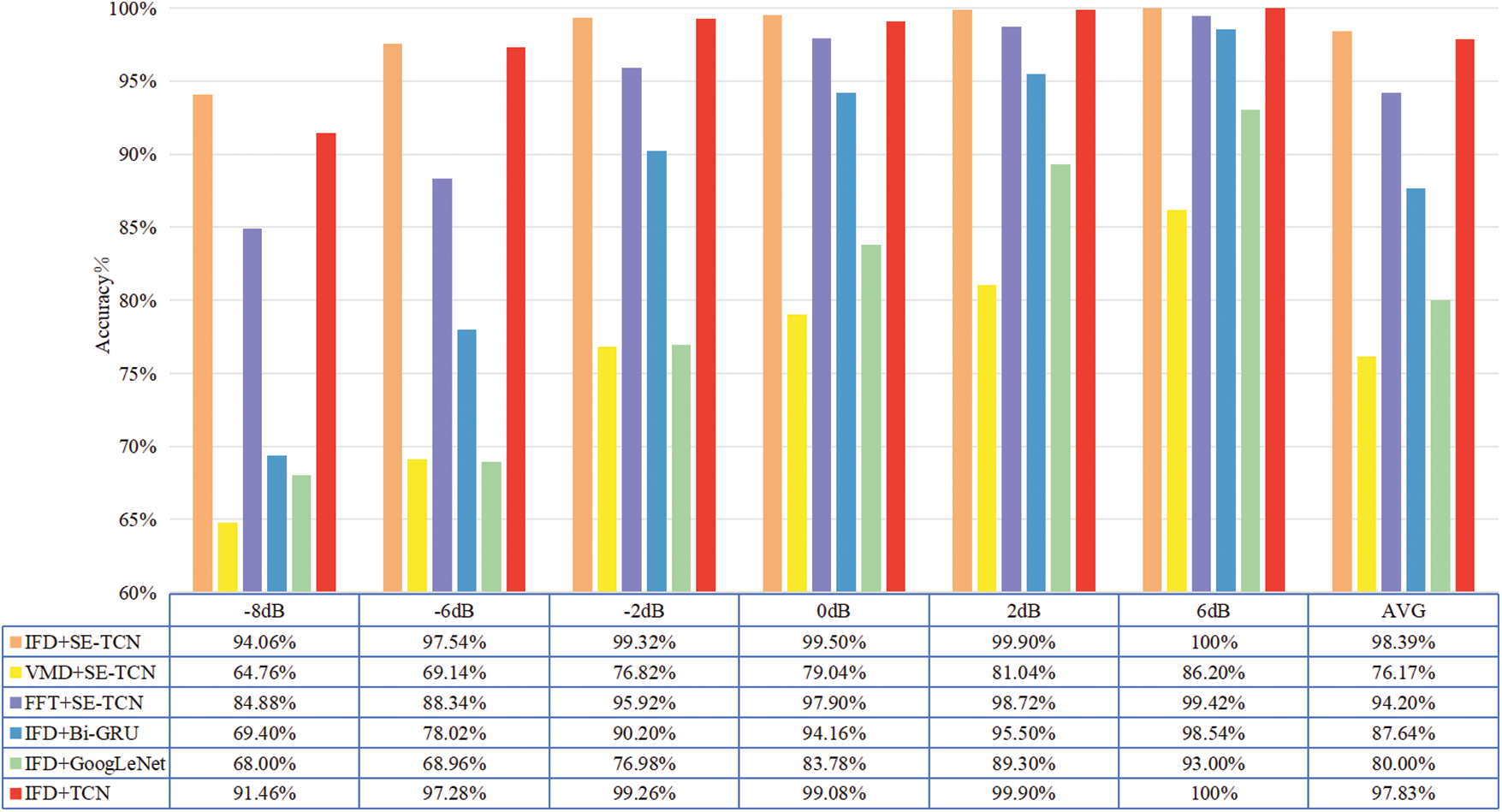
Figure 9: Recognition accuracy under different noise conditions

Fig. 9 shows that when SNR = −8 dB and only one of the FFT and VMD methods are used to process data, the accuracies of the SE-TCN model only reached 64.76% and 84.88%, respectively. These results indicate that signals cannot be distinguished accurately when noise components are present in the original signals. The multiscale information fusion method still achieved an accuracy rate of 94.06% when SNR = −8 dB and up to 100% when SNR = 6 dB. Hence, the data fusion method can greatly reduce the influence of signals from noise. The accuracies of different models obtained using the same dataset IFD differ greatly under the interference of noise. Comparatively speaking, SE-TCN has a much higher accuracy rate than Bi-GRU and GoogLeNet.

The suggested method can achieve greater accuracy under different SNR situations than other methods. This is because the pre-processing of the multiscale data fusion method contains rich features such that when combined with the powerful sequence processing ability of SE-TCN, the suggested method shows a strong antinoise ability.

3.3 Performance Analysis under Variable Load Conditions

The working loads of rotating machinery change during actual operations. When the load changes, the vibration response of bearings will also change, which means that the model must have a strong capacity for generalization to cope with various loads.

This set of experiments tested the adaptability of the proposed method under different loads. In this experiment, analyzed using datasets A, B, and C, one of the datasets was trained first, and the best model was saved, after which it was tested separately with the other two datasets. In Fig. 10, A→B indicates that dataset A is taken as the test set and dataset B as the training set.

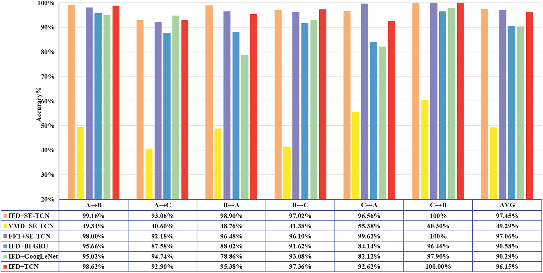
Figure 10: Identification accuracies under variable load conditions

Fig. 10 shows that, among the diagnosis methods, the IFD+SE-TCN method has the highest average accuracy of 97.45%, while those of IFD+Bi-GRU and IFD+GoogLeNet are 90.58% and 90.25%, respectively. Generally, these two models’ accuracy rates are lower than 90% (or even less than 80% in most cases) among six groups of experiments with different loads switching between each other. The average accuracy of SE-TCN, being about 7% higher than that of the other two models, can be attributed to the special structure of the dilated causal convolution and residual connection in the model, which can greatly expand the receptive field. Such expansion allows it to determine the common characteristics of different load signals well and efficiently perform the task of cross-domain self-adaptation under different working conditions.

In addition, even though the accuracy of TCN without SE attention mechanism reached 96.15%, when its load changes (A→C and C→A), the accuracy becomes far lower than that of A→B, B→A, B→C, C→B because the load gap between A and C is large. Therefore, accuracy decreases when significant variations in load occur. Adding the SE attention mechanism not only solves the problem but also improves overall average accuracy by 1.3%. The average accuracies of VMD+SE-TCN and FFT+SE-TCN using only one preprocessing method are 49.29% and 97.06%, which are both lower than that of IFD+SE-TCN. The method using only VMD to process data almost lost its fault diagnosis ability under variable load conditions.

Compared to Figs. 9 and 10, FFT+SE-TCN performs well in the variable load experiments but poorly in the case of noise interference, while IFD+TCN performs well in the case of noise but poorly in the case of variable load. Hence, the multiscale information fusion method combining FFT and VMD can lessen the impact of noise on the model, and adding the SE attention can enhance the adaptive capability of the model.

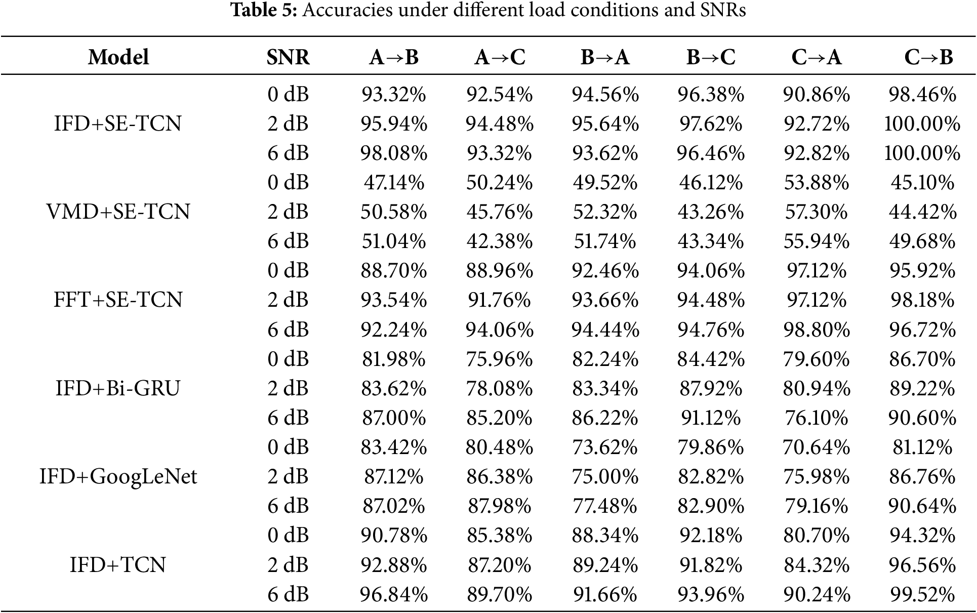
Finally, this paper verified the comprehensive ability of the model by adding 0, 2, and 6 dB noise to each of the three datasets and then conducting variable load experiments that are more in line with actual industrial production environments. Table 5 shows the accuracies of different methods under varying load conditions and SNRs. As shown in the table, the IFD+SE-TCN method has the best performance among all the methods, achieving high accuracy under the three SNRs, thus proving its highly stable characteristic. It also alleviates the problem of decreased accuracy caused by excessive load changes.

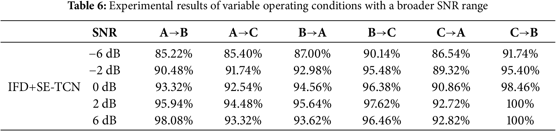
Next, noise with a larger SNR range was added to the data, and then used the IFD+SE-TCN method for variable load experiments. The results in Table 6 indicate that, although the accuracy may decrease as the influence of noise increases, the overall accuracy of the proposed method is still relatively high. This finding reveals that the IFD+SE-TCN method can still accurately diagnose fault under variable operating conditions, even with high SNRs.

3.4 Performance Analysis of Models under Variable Operating Conditions Using the PU Bearing Dataset

In this section, variable condition experiments were conducted using the PU-bearing dataset to demonstrate the generalization of the proposed method further. In this public dataset, the PU-data acquisition platform consists of (1) an electric motor, (2) a torque measurement shaft, (3) a bearing testing module, (4) a flywheel, and (5) a load motor. The tested bearing was a rolling bearing model 6203. The sampling frequency of the accelerometer is 64 kHz. The damaged areas included the inner ring, outer ring, and inner outer ring composite. The same dataset creation method described above is used to process the PU-bearing dataset. The data included three operating conditions, as shown in Table 7.

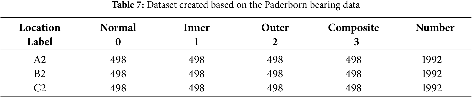
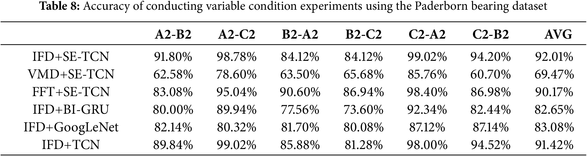
Table 8 shows that, even after changing the dataset, the IFD+SE-TCN model still has strong adaptability to changing operating conditions with an accuracy of 92.01%. This result indicates that the proposed method is almost unaffected by changes in data sources and can adapt to different practical environments while retaining its strong generalization ability.

4  Conclusions

This paper aims to explore the actual working conditions of rolling bearings. The working conditions of rolling bearings are complex, varied, and changeable. In situations where noise interference is present, the vibration signals’ fault features are difficult to extract, and the accuracy of the classification model is low. A rolling bearing fault diagnostic method based on FFT-VMD multiscale information fusion and SE-TCN model was thus proposed. Combining the preprocessing methods of FFT and VMD obtained the original signal’s frequency domain component and the inherent mode function with different center frequencies. Then, the new data containing more fault signatures were obtained. Finally, the new data were inputted into the SE-TCN for fault diagnosis. The following conclusions were drawn:

(1) Compared with a single processing method, the proposed FFT-VMD data preprocessing method retains the correlation between different time intervals of signals and rich fault characteristics. It can effectively identify and reduce random fluctuations and non-target signal components in the data, as proven by an antinoise experiment. When SNR = −8 dB, the accuracies of the other control experiments are low, while that of the SE-TCN method can reach 94.06%.

(2) Comparing the performance of different models, SE-TCN has a higher accuracy than Bi-GRU and GoogLeNet in experiments involving antinoise interference and variable operating conditions. The findings demonstrate that the suggested model can learn the prominent trends of the data and adapt to major changes in the data. The findings also demonstrate the proposed model’s strong generalization ability.

(3) Adding an SE module to the TCN can promote the effective fusion of features at different scales. Based on different inputs, the attention weight can be adjusted dynamically to capture global and local data patterns better and enhance adaptability to various complex scenes.

This method has excellent accuracy under variable operating conditions, noise interference, and a combination of both. In practice, obtaining bearing fault samples can be difficult. Thus, in future research, we will continue to improve the model to adapt to conditions involving small sample sizes.

Acknowledgement: None.

Funding Statement: This work was supported by Handan Science and Technology Research and Development Plan Project under Grant no. 23422901031 and Key Laboratory of Intelligent Industrial Equipment Technology of Hebei Province (Hebei University of Engineering) under Grant no. 202206.

Author Contributions: The authors confirm contribution to the paper as follows: Methodology: Chaozhi Cai, Yuqi Ren; Software: Yuqi Ren, Yingfang Xue; draft manuscript preparation: Chaozhi Cai, Yuqi Ren, Yingfang Xue; Data curation: Yuqi Ren, Jianhua Ren; Validation: Chaozhi Cai, Jianhua Ren. All authors reviewed the results and approved the final version of the manuscript.

Availability of Data and Materials: Paderborn University Bearing Dataset Available from: Index of /kat/BearingDataCenter (uni-paderborn.de) (accessed on 09 December 2024) Case Western Reserve University Bearing Dataset Available from: Bearing Data Center | Case School of Engineering | Case Western Reserve University (accessed on 09 December 2024).

Ethics Approval: Not applicable.

Conflicts of Interest: The authors declare no conflicts of interest to report regarding the present study.

References

1. Zhang X, Zhao B, Lin Y. Machine learning based bearing fault diagnosis using the case western reserve university data: a review. IEEE Access. 2021;9:155598–608. doi:10.1109/ACCESS.2021.3128669. [Google Scholar] [CrossRef]

2. Chauhan S, Vashishtha G, Zimroz R, Kumar R, Gupta MK. Optimal filter design using mountain gazelle optimizer driven by novel sparsity index and its application to fault diagnosis. Appl Acoust. 2024;225:110200. doi:10.1016/j.apacoust.2024.110200. [Google Scholar] [CrossRef]

3. Vashishtha G, Chauhan S, Zimroz R, Kumar R, Gupta MK. Optimization of spectral kurtosis-based filtering through flow direction algorithm for early fault detection. Measurement. 2025;241:115737. doi:10.1016/j.measurement.2024.115737. [Google Scholar] [CrossRef]

4. Zhang Q, Deng L. An intelligent fault diagnosis method of rolling bearings based on short-time Fourier transform and convolutional neural network. J Fail Anal Prev. 2023;23(2):795–811. doi:10.1007/s11668-023-01616-9. [Google Scholar] [CrossRef]

5. Lou X, Loparo KA. Bearing fault diagnosis based on wavelet transform and fuzzy inference. Mech Syst Sig Process. 2004;18(5):1077–95. doi:10.1016/s0888-3270(03)00077-3. [Google Scholar] [CrossRef]

6. Boudraa AO, Cexus JC. EMD-based signal filtering. IEEE Trans Instrum Meas. 2007;56(6):2196–202. doi:10.1109/TIM.2007.907967. [Google Scholar] [CrossRef]

7. Su W, Wang F, Zhu H, Zhang Z, Guo Z. Rolling element bearing faults diagnosis based on optimal Morlet wavelet filter and autocorrelation enhancement. Mech Syst Sig Process. 2010;24(5):1458–72. doi:10.1016/j.ymssp.2009.11.011. [Google Scholar] [CrossRef]

8. Zhang X, Liu Z, Wang J, Wang J. Time-frequency analysis for bearing fault diagnosis using multiple Q-factor Gabor wavelets. ISA Trans. 2019;87:225–34. doi:10.1016/j.isatra.2018.11.033. [Google Scholar] [PubMed] [CrossRef]

9. Sun Y, Li S, Wang X. Bearing fault diagnosis based on EMD and improved Chebyshev distance in SDP image. Measurement. 2021;176:109100. doi:10.1016/j.measurement.2021.109100. [Google Scholar] [CrossRef]

10. Wu Z, Huang NE. Ensemble empirical mode decomposition: a noise-assisted data analysis method. Adv Data Sci Adapt. 2009;1(1):1–41. doi:10.1142/S1793536909000047. [Google Scholar] [CrossRef]

11. Lei Y, He Z, Zi Y. Application of the EEMD method to rotor fault diagnosis of rotating machinery. Mech Syst Sig Process. 2009;23(4):1327–38. doi:10.1016/j.ymssp.2008.11.005. [Google Scholar] [CrossRef]

12. Torres ME, Colominas MA, Schlotthauer G, Flandrin P. A complete ensemble empirical mode decomposition with adaptive noise. In: 2011 IEEE International Conference on Acoustics, Speech and Signal Processing (ICASSP); 2011 May 22–27; Prague, Czech Republic: IEEE. p. 4144–47. [Google Scholar]

13. Zhang D, Wang Y, Jiang Y, Zhao T, Xu H, Qian P, et al. A novel wind turbine rolling element bearing fault diagnosis method based on CEEMDAN and improved TFR demodulation analysis. Energies. 2024;17(4):819. doi:10.3390/en17040819. [Google Scholar] [CrossRef]

14. Zhang W, Li C, Peng G, Chen Y, Zhang Z. A deep convolutional neural network with new training methods for bearing fault diagnosis under noisy environment and different working load. Mech Syst Sig Process. 2018;100:439–53. doi:10.1016/j.ymssp.2017.06.022. [Google Scholar] [CrossRef]

15. Wang F, Jiang H, Shao H, Duan W, Wu S. An adaptive deep convolutional neural network for rolling bearing fault diagnosis. Meas Sci Technol. 2017;28(9):095005. doi:10.1088/1361-6501/aa6e22. [Google Scholar] [CrossRef]

16. Han T, Zhang L, Yin Z, Tan AC. Rolling bearing fault diagnosis with combined convolutional neural networks and support vector machine. Measurement. 2021;177(1):109022. doi:10.1016/j.measurement.2021.109022. [Google Scholar] [CrossRef]

17. Habbouche H, Amirat Y, Benkedjouh T, Benbouzid M. Bearing fault event-triggered diagnosis using a variational mode decomposition-based machine learning approach. IEEE Trans Energy Conver. 2021;37(1):466–74. doi:10.1109/TEC.2021.3085909. [Google Scholar] [CrossRef]

18. Liu H, Zhou J, Zheng Y, Jiang W, Zhang Y. Fault diagnosis of rolling bearings with recurrent neural network-based autoencoders. ISA Trans. 2018;77:167–78. doi:10.1016/j.isatra.2018.04.005. [Google Scholar] [PubMed] [CrossRef]

19. Sabir R, Rosato D, Hartmann S, Guehmann C. LSTM based bearing fault diagnosis of electrical machines using motor current signal. In: 2019 18th IEEE International Conference on Machine Learning and Applications (ICMLA); 2019 Dec 16–19; Boca Raton, FL, USA: IEEE. p. 613–18. [Google Scholar]

20. Hao S, Ge FX, Li Y, Jiang J. Multisensor bearing fault diagnosis based on one-dimensional convolutional long short-term memory networks. Measurement. 2020;159:107802. doi:10.1016/j.measurement.2020.107802. [Google Scholar] [CrossRef]

21. Ni Q, Ji JC, Halkon B, Nandi AK. Physics-informed residual network (PIResNet) for rolling element bearing fault diagnostics. Mech Syst Sig Process. 2023;200:110544. doi:10.1016/j.ymssp.2023.110544. [Google Scholar] [CrossRef]

22. Zhang K, Wang J, Shi H, Zhang X, Tang Y. A fault diagnosis method based on improved convolutional neural network for bearings under variable working conditions. Measurement. 2021;182(1):109749. doi:10.1016/j.measurement.2021.109749. [Google Scholar] [CrossRef]

23. Zhou F, Zhou W, Chen D, Wen C. Rolling bearing real time fault diagnosis using convolutional neural network. In: 2019 Chinese Control And Decision Conference (CCDC); 2019 Jun 3–5; Nanchang, China: IEEE. p. 377–82. [Google Scholar]

24. Yan J, Kan J, Luo H. Rolling bearing fault diagnosis based on Markov transition field and residual network. Sensors. 2022;22(10):3936. doi:10.3390/s22103936. [Google Scholar] [PubMed] [CrossRef]

25. Shen J, Wu Z, Cao Y, Zhang Q, Cui Y. Research on fault diagnosis of rolling bearing based on gramian angular field and lightweight model. Sensors. 2024;24(18):5952. doi:10.3390/s24185952. [Google Scholar] [PubMed] [CrossRef]

26. Ye M, Yan X, Chen N, Jia M. Intelligent fault diagnosis of rolling bearing using variational mode extraction and improved one-dimensional convolutional neural network. Appl Acoust. 2023;202:109143. doi:10.1016/j.apacoust.2022.109143. [Google Scholar] [CrossRef]

27. Bai S, Kolter JZ, Koltun V. An empirical evaluation of generic convolutional and recurrent networks for sequence modeling; 2018 [cited 2024 Nov 4]. Available from: https://arxiv.org/abs/1803.01271. [Google Scholar]

28. Hu J, Shen L, Sun G. Squeeze-and-excitation networks. In: Proceedings of the IEEE Conference on Computer Vision and Pattern Recognition (CVPR); 2018 Jun 18–22; Salt Lake City, UT, USA: Computer Vision Foundation. p. 7132–41. [Google Scholar]

29. Sikder N, Bhakta K, Al Nahid A, IsIam MM. Fault diagnosis of motor bearing using ensemble learning algorithm with FFT-based preprocessing. In: 2019 International Conference on Robotics, Electrical and Signal Processing Techniques (ICREST); 2019 Jan 10–12; Dhaka, Bangladesh: IEEE. p. 564–69. [Google Scholar]

30. Liu C, Zhu L, Ni C. Chatter detection in milling process based on VMD and energy entropy. Mech Syst Sig Process. 2018;105:169–82. doi:10.1016/j.ymssp.2017.11.046. [Google Scholar] [CrossRef]