Rolling Bearing Fault Detection Based on Self-Adaptive Wasserstein Dual Generative Adversarial Networks and Feature Fusion under Small Sample Conditions

1  Introduction

As an indispensable support and transmission component in industrial equipment, the health condition of rolling bearings is directly correlated with the operational efficiency and safety of the entire system [1]. Therefore, timely and accurate fault diagnosis of rolling bearings is regarded not only as a crucial guarantee for the safe operation of main bearings but also as a key component in ensuring the efficient and reliable operation of the entire industrial system. Especially in areas requiring high reliability, such as power generation, railway transportation and aviation, the prevention and timely diagnosis of bearing failures are essential. Meanwhile, with the promotion of Industry 4.0 and the application of intelligent fault detection technology, real-time monitoring, and data analysis are possible [2,3]. In recent years, with the advancement of intelligent diagnostic methods, the application of deep learning in the field of fault diagnosis has been steadily increasing. The implementation of deep learning technologies allows for the development of more accurate and efficient fault diagnosis systems, remarkably enhancing the accuracy of fault diagnosis [4–7]. However, the field of fault diagnosis founded on deep learning currently faces two critical issues.

First, the efficient operation of deep learning models is often highly contingent upon a set of training sets with sufficient data [8]. However, the fault data collected under different machine states often face the problem of insufficient samples due to the complexity of machine operation and the random nature of failures in real industrial environments [9–11], especially when the amount of data under the fault state is much less than that under the normal operation state [12–14]. This phenomenon of inadequate sample size results in a diminished recognition capability of the model for minority classes, thereby affecting the accuracy of fault diagnosis and the generalization ability of the model. Currently, the predominant research approaches can be broadly categorized into knowledge-level and data-level studies. Knowledge-level approaches encompass strategies such as transfer learning and metal-earning, where transfer learning seeks to leverage data and knowledge from the source domain to facilitate learning in the target domain. If the distribution of data between the source and target domains deviates considerably, transfer learning may not achieve satisfactory results [15–18]. Meta-learning demonstrates remarkable potential in certain scenarios by learning efficient deep learning algorithms across various tasks [19–21]. However, the generalization ability of its metaknowledge may be somewhat constrained where data is extremely scarce. Data-level approaches encompass techniques such as synthetic minority oversampling technique (SMOTE) and generative adversarial network (GAN). Inspired by random oversampling, Chawla et al. [22] proposed the SMOTE, which increases the number of existing minority class samples by interpolating them. However, its effectiveness is constrained due to the introduction of noise and the challenges associated with accurately capturing complex data distributions. Accordingly, the utilization of GAN at the data level to synthesize minority classes for augmenting the dataset is considered the optimal approach for enhancing classifier performance. Goodfellow et al. [23] proposed a data synthesis model known as GAN, where the generator and discriminator are trained through a game-theoretic framework to generate realistic data samples. As the study progressed, Radford et al. [24] established the deep convolutional generative adversarial network (DCGAN) by substituting conventional multilayer neural networks with convolutional neural network (CNN). This convolutional variant of GAN demonstrated improved training performance across various datasets. Li et al. [25] presented an advanced version of GAN, i.e., the Wasserstein DCGAN (WDCGAN), capable of generating data from one-dimensional power grid datasets. The generated data serve as input for intelligent diagnostic models, facilitating small-sample anomaly classification. Importantly, the generated data of the WDCGAN exhibit similarity to real data, effectively stabilizing the training process.

Moreover, the majority of current diagnostic models primarily rely on unidimensional single-information inputs, resulting in insufficient sample coverage and consequently diminishing generalization capability and diagnostic accuracy of the model. Therefore, the limitations of diagnostic models stemming from single-information inputs are evident, necessitating the incorporation of multidimensional information to enhance diagnostic accuracy and comprehensiveness [26,27]. In recent years, CNN have demonstrated remarkable advantages in equipment fault identification due to their superior automatic feature extraction and pattern recognition capabilities. Efficient and accurate diagnostics can be achieved by CNN through the direct processing of input two-dimensional images or vibration signals [28–31]. Chen et al. [32] transformed the original one-dimensional vibration signals into a two-dimensional matrix structure and employed CNN for fault identification. Gao et al. [33] converted one-dimensional vibration signals into a time-frequency grayscale map and achieved the diagnosis classification of faults through CNN. However, vibration signals, as one-dimensional time series, exhibit certain temporal correlations and continuity characteristics. The conversion of one-dimensional data into two-dimensional arrays can disrupt the spatial correlation of the signals, leading to the loss of one-dimensional waveform feature information [34]. Therefore, extensive research has been conducted by scholars domestically and internationally on one-dimensional convolutional neural networks (1DCNN) due to the uniqueness of one-dimensional time series. Ye et al. [35] designed a diagnostic method that successfully improves recognition accuracy by integrating variational modal extraction with an enhanced 1DCNN. While this approach preserves spatial information and waveform features by utilizing one-dimensional vibration signals as input data, it neglects certain fault characteristics in the frequency domain. Subsequently, researchers have introduced dual-channel CNN, utilizing the frequency spectrum and time-frequency representations of the original vibration signals as input for diagnostic detection, thereby enabling fault diagnosis [36]. The method incorporates frequency domain feature extraction. However, it fails to extract the information effectively from the original time series and the structural information manifesting in the time domain. Furthermore, existing diagnostic methods based on feature fusion do not fundamentally address the challenge of inadequate sample size. Thus, further studies on small-sample fault diagnosis for feature fusion are required in the future.

In response to the emergence of the aforementioned issues, a small-sample diagnosis method based on self-adaptive Wasserstein dual generative adversarial networks and feature fusion is proposed in this study, and the main contributions can be summarized as follows:

1.    This method utilized continuous wavelet transform and grayscale image transformation, incorporating one-dimensional vibration signals, time-frequency images, and grayscale images as input data, which include the waveform features, structural features, and time-frequency features of the one-dimensional signals.

2.    Dual models of one-dimensional and two-dimensional WDCGAN were constructed for the sample augmentation of multidimensional data, thereby generating an augmented new dataset. Additionally, a self-adaptive loss threshold control training (SALTCT) strategy was incorporated into the model to achieve a stable training process. Instance normalization (IN) is substituted for batch normalization (BN) to preserve the independence of each sample and thus extract all the important information contained in the data.

3.    Within the diagnostic classification module, a method known as multidimensional feature fusion convolutional neural network (MDFFCNN) was devised to facilitate in-depth feature extraction and fusion of three categories of fault features, thereby achieving efficient and precise fault diagnosis.

This paper is structured as follows: Section 2 offers a comprehensive overview of the theoretical background underpinning the method. In Section 3, the proposed method is described in detail. Section 4 presents the experimental results obtained through the application of this method. Finally, Section 5 provides a conclusion to this study.

2  Theoretical Background

2.1 GAN and Its Improved Models

As an unsupervised deep learning model, GAN is fundamentally based on the principles of zero-sum game theory. The network comprises a generator (G) and a discriminator (D), and through the iterative optimization involving adversarial training and backpropagation between G and D, the model ultimately attains Nash equilibrium, resulting in the generation of realistic and diverse data. The objective function of GAN is defined as follows:

minGmaxDV(D,G)=Ex∼Pr(x)(x)log⁡D(x)+Ez∼Pz(z)[log⁡(1−D(G(z)))],(1)

where x represents the real data sampled from the true data distribution Pr. The objective of the discriminator is to maximize the probability that input samples belong to the real data distribution, while the aim of the generator is to ensure that the distribution of generated data closely approximates that of the real samples, with its input being a random noise vector z sampled from a normal distribution Pz(z).

DCGAN replaces the conventional multilayer neural networks with GAN based on CNNs, and this convolutional variant of GAN demonstrates stable training performance across numerous datasets. Wasserstein GAN (WGAN) [37] enhances the training stability of GANs and the diversity of generated samples by introducing the Wasserstein distance as a metric and imposing a Lipschitz constraint on the discriminator, with its objective function illustrated in Eq. (2):

minGmaxD∈ΔV(D,G)=Ex∼Pr[D(x)]−Ex∼Pg[D(x)],(2)

where Pg is the generated data distribution defined by the implicit generative model G, and Δ is the 1−Lipschitz condition. The gradient penalty (GP) method is introduced in WGAN-GP to overcome the limitations associated with weight clipping in WGAN [38]. Specifically, a gradient-related penalty term is incorporated into the loss function of the discriminator in WGAN-GP, thereby indirectly enforcing the Lipschitz constraint. This enhancement not only simplifies the training process but also improves the stability of WGAN and the quality of the generated samples. The objective function of WGAN-GP is shown in Eq. (3):

minGmaxDV(D,G)=−Ex∼Pr[D(x)]+Ex^∼Pg[D(x^)]+λEx^∼Px^[(∥∇x^D(x^)∥2−1)2],(3)

where λ represents the GP coefficient, x^ denotes the random interpolation sampling along the line connecting Pr and Pg, and ||•|| indicates the L2 norm of the gradient.

In this study, a data generation model named WDCGAN with GP (WDCGAN-GP) was employed. The proposed model incorporates part of the CNN architectures from DCGAN into the framework of WGAN-GP. By optimizing the model architecture and incorporating convolutional layers alongside feature extraction capabilities, this model is designed to capture the diversity within the data while reducing computational costs and enhancing training efficiency.

2.2 Instance Normalization

Instance Normalization (IN) is a widely used technique, particularly in tasks such as image generation and style transfer. It operates by computing the mean and standard deviation for each channel of an input sample, normalizing the sample based on these statistics. This method can effectively remove unnecessary style information from the image by independently adjusting the statistics of each sample, thereby capturing content features [39]. The expression for IN is delineated in Eq. (4).

{ynij=xnij−μniσni2+ε,μni=1L∑l=1Lxnij,σni2=1L∑l=1L(xnij−μni)2,(4)

where x is the input tensor containing N signal samples (x∈RN×C×L). xnij represents the nij-th element; C, N, L, and ε respectively represent the number of channels, the number of samples in batch, the sample length, and the numerical stability coefficient.

3  Proposed Method

3.1 Multidimensional Data Enhancement Model

One-dimensional and two-dimensional Wasserstein DCGANS (1DWDCGAN and 2DWDCGAN) are constructed in this study as generative adversarial models. The model architecture and key parameters are presented in Tables 1 and 2. The integration of certain components of the DCGAN is incorporated into the model based on WGAN-GP. In this study, convolutional and inverse convolutional layers are used in the generator and discriminator, respectively. Convolutional layers help extract localized features from the signal and gradually learn high-level features through multiple layers of convolution. In the generator, the inverse convolutional layer is used to map the low-dimensional latent vectors back into the signal space, thus generating a more accurate orientation signal. With this design, important data features in the signal can be captured while generating representative fault signals. Rectified linear unit (ReLU) is used as the activation function of the generator, and the tanh activation function in the output layer is employed to ensure that the generated signals remain within a reasonable range and fit the distribution of the real signals. The use of leaky ReLU as the activation function of the discriminator effectively mitigates the gradient vanishing problem while improving the performance of the model under different input signals. Given that each data point within a sample contains considerable unique information, the application of BN may lead to the loss of distinctive detailed features in individual samples. BN standardizes the distribution of data across an entire batch and may lead to the loss of distinctive detailed features in each generated sample. As a result, IN is substituted for BN to preserve the independence of each sample.

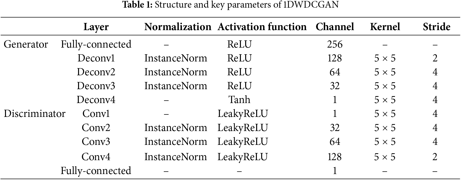
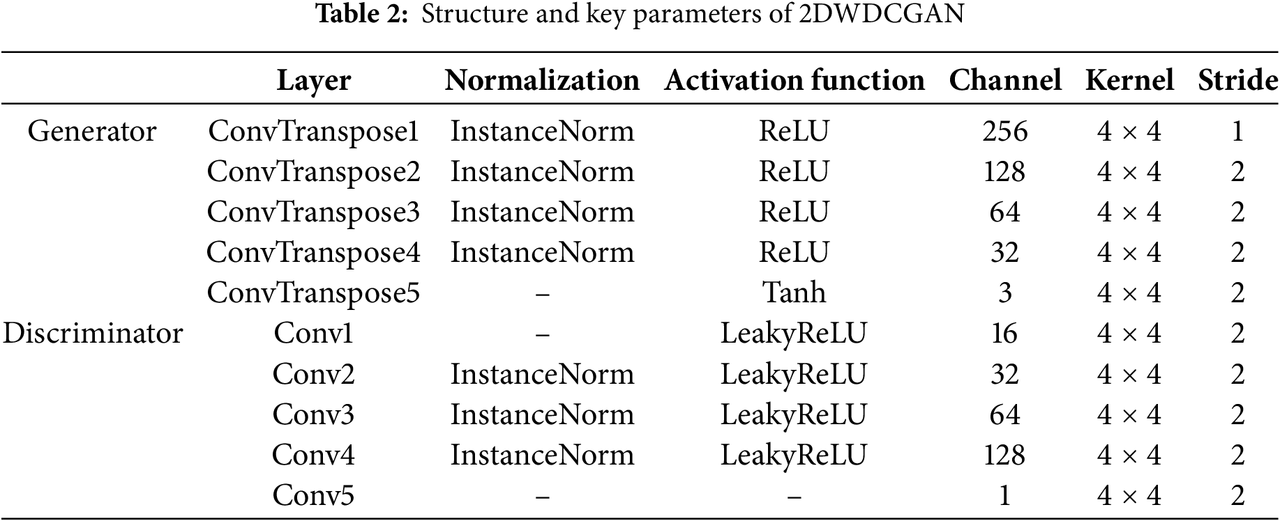
The architecture of the 1DWDCGAN is based on a one-dimensional convolutional structure, which facilitates the extraction of deep features for the generator and discriminator. Fully connected layers serve as the input layer of the generator and the output layer of the discriminator. The batch size is set to 5, and the generator and discriminator use the Adam optimizer and a learning rate of 0.0002, with 30,000 iterations. By contrast, the 2DWDCGAN model adopts a two-dimensional convolutional approach, whereby a 100-dimensional random noise vector, consistent with a Gaussian distribution, is mapped to various convolutional feature maps, which culminate in the generation of two-dimensional images. The batch size is set to 32. For the optimizer, Adam is adopted for the generator and discriminator, and the learning rate is 0.0002. The number of iterations is 500.

A self-adaptive training strategy based on loss threshold control, termed SALTCT, is introduced to ensure that the model converges stably and approaches a Nash equilibrium state. This strategy regulates the training intensity between the generator and the discriminator to achieve a balance in their learning capacities, thereby mitigating oscillatory phenomena during the training process and enhancing model stability. The mathematical expression is shown as follows:

ΔL=|LG|−|LD|,(5)

train G={TrueifΔL>TFalseotherwise,(6)

trainD={TrueifΔL<−TFalseotherwise,(7)

where ΔL is the loss difference; LG, LD are the generator loss and discriminator loss, respectively. Eqs. (6) and (7) denote the training conditions for the generator and discriminator, respectively, and T is the preset threshold. A threshold T of 1.5 was established in advance to assess the acceptable range of discrepancy in the loss function values between the generator and discriminator during each iteration. In the original training loop, the parameters of the generator and discriminator are updated during each iteration. Following the updates, the loss values for both are computed, and the difference ΔL is calculated. ΔL > T indicates that the discriminator may be too strong or the generator is too weak. Hence, additional training iterations are conducted while keeping the parameters of the other network fixed, with the generator being trained an additional five times. Conversely, if ΔL < −T, the discriminator is trained an additional five times. After each additional iteration, the loss discrepancy ΔL is recalculated until it returns to the range of [−T, T]. Once the loss discrepancy meets the threshold condition, the current state of training is deemed stable, and the original training loop is continued.

3.2 Novel Multidimensional Feature Fusion Fault Diagnosis Method

To address the low diagnostic accuracy and insufficient generalization ability of the model caused by the limitations of single-dimensional and single-information input data characteristics, this study introduces an innovative intelligent diagnostic model, namely, MDFFCNN. It incorporates one-dimensional vibration signals, grayscale images, and time-frequency images as simultaneous inputs. A 1DCNN and two-dimensional convolutional neural network (2DCNN) modules are employed to extract deep features concurrently from the three types of input samples, which are then fused into a multidimensional, multiscale deep composite feature representation that encompasses the original signal waveform features, structured features, and time-frequency characteristics. In the fusion process, a feature concatenation method is adopted to merge one-dimensional signal features with two sets of two-dimensional image features. The features of each channel can model the signal from different dimensions. By concatenating these features, the multilevel information of the signal can be captured, and rich and comprehensive composite features are formed. This approach enables the model to consider multidimensional information such as time, space, and frequency comprehensively, thereby improving diagnostic performance. Ultimately, an intelligent fault diagnosis for small samples with multidimensional input is achieved, with the specific model architecture and key parameters illustrated in Fig. 1.

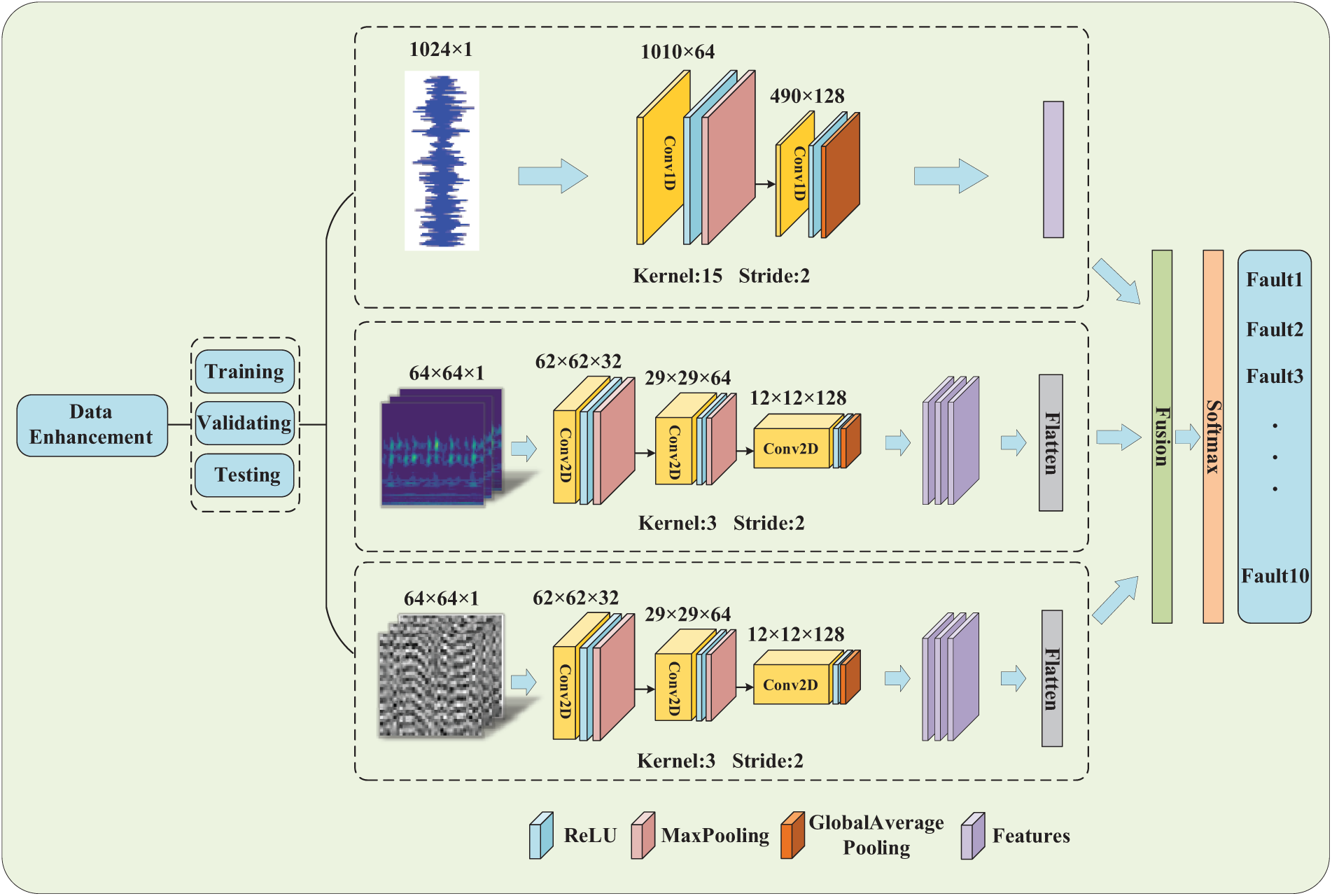
Figure 1: Structure and key parameters of MDFFCNN

In the MDFFCNN model, the convolutional layer integrates one-dimensional and two-dimensional convolution operations to extract fault features. To introduce nonlinear mapping capabilities, ReLU is employed as the activation function. A maximum pooling layer is added after each convolution module to reduce the dimensionality of the output features, defined as follows:

ykij=max(p,q)∈Rijxxpq,(8)

where ykij denotes the maximum pooling output value of the pooling region Rij associated with the k-th feature map; xxpq represents the element located at (p, q) within the pooling region Rij.

In the final convolutional module, global average pooling (GAP) is employed to replace the fully connected layer, with the aim of capturing global feature information of the model while minimizing the number of parameters. This enables the model to prioritize global features across the entire feature map, rather than being limited to local regions, thereby mitigating the overfitting phenomenon typically induced by the extensive weight parameters present in traditional fully connected layers. Let F denote an input feature map with dimensions H × W × C, where H, W, and C correspond to the height, width, and number of channels of the feature map, respectively. The operation of GAP can be expressed by the following equation:

GAP(F)=[1H×W∑i=1H∑j=1WF(i,j,c)]c=1C,(9)

where F (i, j, c) denotes the value of channel c at position (i, j) in the feature map F, and the output of GAP(F) is a vector of length C, where each element represents the global average of the corresponding channel.

In the 2DCNN module, the extracted time-frequency and structured features are flattened into one-dimensional features using a flattening layer, facilitating the integration of deep features of different dimensions at the fusion layer. The operational steps of the flattening layer are illustrated in Eqs. (10) and (11).

Qi=(s11⋯s1h⋮⋯⋱sh1⋯shh),(10)

qiT=flatten(Qi)=[s11,⋯,s1h,⋯,sh1,⋯,shh],(11)

where Qi denotes the two-dimensional feature map extracted by the 2DCNN with a size of h × h, Shh represents the feature value at the h-th row and h-th column, and qiT signifies the flattened feature vector. The definition of the fusion layer is as follows:

diT=FF(qi1,qi2,qi3)=[s111,⋯,shh1,s112,⋯,shh2,⋯,s113,⋯,shh3],(12)

where qi1 is the one-dimensional feature vector of the original signal, while qi2 and qi3 are the time-frequency and structured two-dimensional feature vectors extracted after processing with Continuous wavelet transform (CWT) and grayscale image transform (GIT), respectively [40–42]. S…1, S…2 and S…3 represent the individual feature values of qi1, qi2, and qi3, respectively. Finally, a SoftMax layer is employed as the classifier to categorize the multidimensional feature vector obtained after deep feature fusion, thereby achieving fault diagnosis based on multidimensional feature integration. The batch size is set to 64, utilizing the Adam optimizer with a learning rate of 0.001.

3.3 Diagnostic Framework Process of the Proposed Method

A method for small-sample diagnosis based on self-adaptive Wasserstein dual generative adversarial network and feature fusion is proposed to address the issue of inadequate sample size prevalent in industrial applications and the challenges of accurate diagnosis caused by the limitations of single information input in intelligent diagnostic models. The overall framework of this method is illustrated in Fig. 2 and consists of three primary stages.

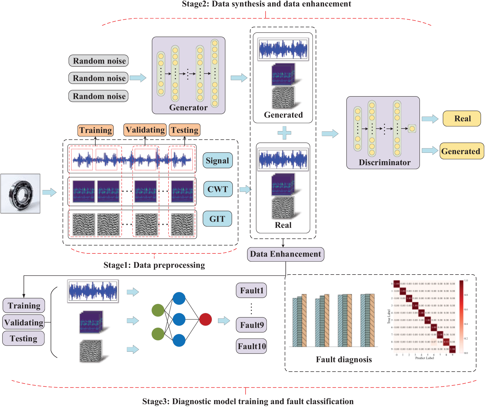
Figure 2: The framework of the proposed method

Stage 1: The continuous bearing vibration signals that are collected are segmented into multiple samples based on predefined time windows and normalized. The CWT and GIT preprocessing methods are applied to convert the raw signals into time-frequency and grayscale images, respectively. The one-dimensional raw vibration signals and the resulting two-dimensional images are divided into training, validation, and test sets in a 7:2:1 ratio. Independent validation and test datasets are employed to effectively mitigate the risk of overfitting and evaluate the performance of the model on unseen data.

Stage 2: 1D-2DWDCGAN are constructed as data synthesis models, incorporating the SALTCT strategy to enhance model convergence speed. Subsequently, these two models are employed to synthesize samples of one-dimensional vibration signals, grayscale images, and time-frequency images with various data augmentation ratios. The synthesized data, along with the real data, are utilized as inputs for the subsequent diagnostic models, thereby effectively augmenting the dataset.

Stage 3: The MDFFCNN model is utilized for fault diagnosis detection, with different ratios of enhanced data used as input during training. Multidimensional convolutional layers are employed to extract the raw signal waveform features, structured features, and time-frequency characteristics. A fusion layer is used to concatenate and integrate deep features from different convolutional paths. During the testing phase, accurate classification of unknown samples is performed, ultimately achieving intelligent fault diagnosis for small samples with multidimensional inputs.

4  Experimental Verification

4.1 Dataset Description and Preprocessing

The performance and effectiveness of the diagnostic method proposed in this study were validated by conducting evaluations on datasets under the 1HP operating condition from the Case Western Reserve University (CWRU) bearing dataset [43] and data collected from the bearing fault simulation experimental platform developed by our research group. The testing platform and fault types are shown in Fig. 3.

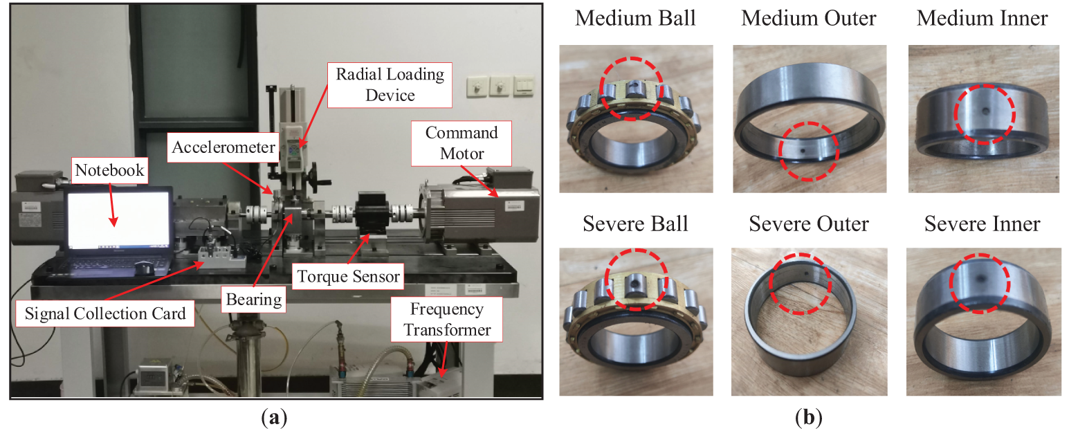
Figure 3: Experimental platform for rolling bearing failure simulation: (a) Bearing failure simulation experiment platform, (b) Types of bearing faults

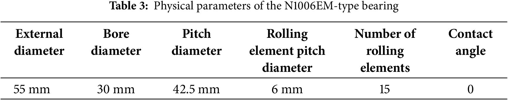
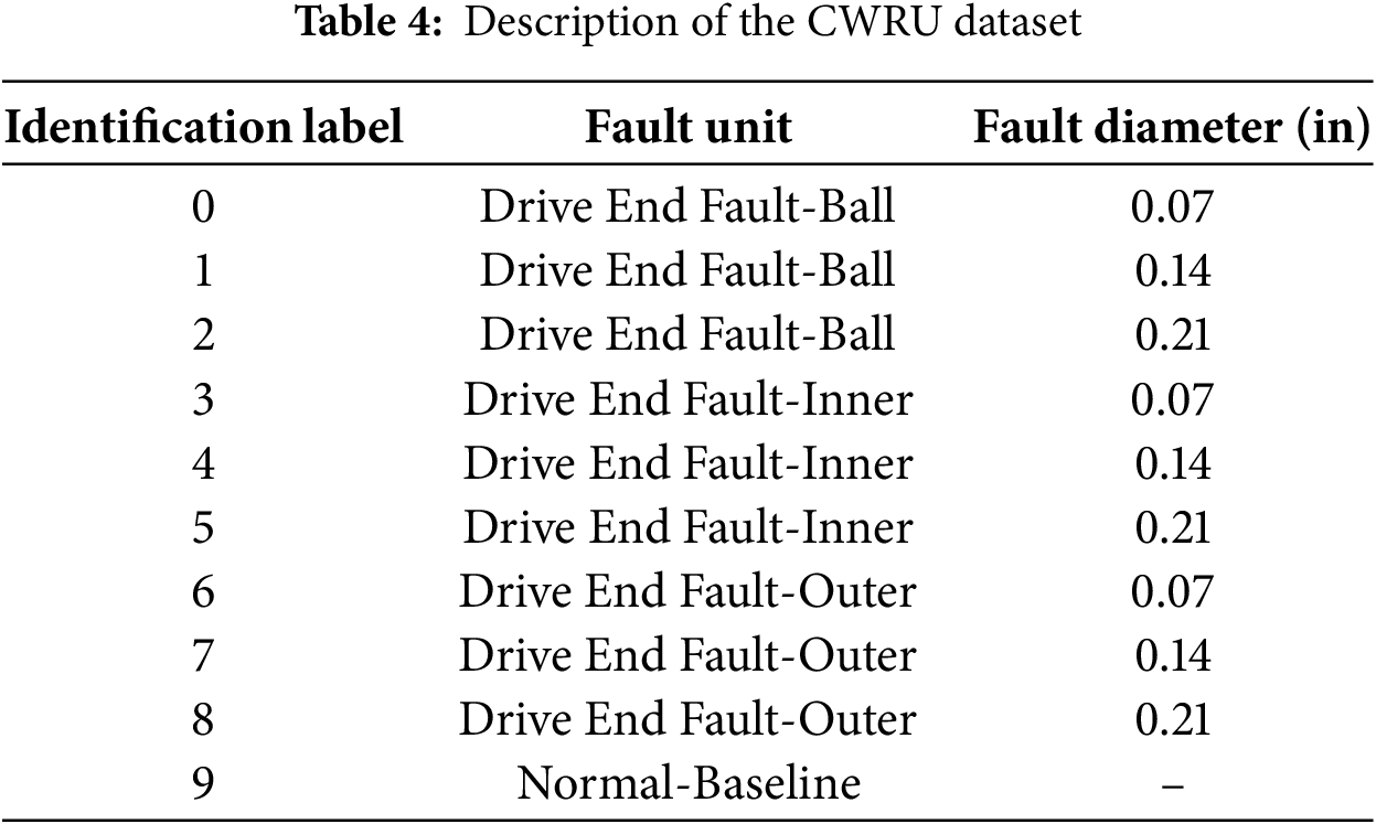
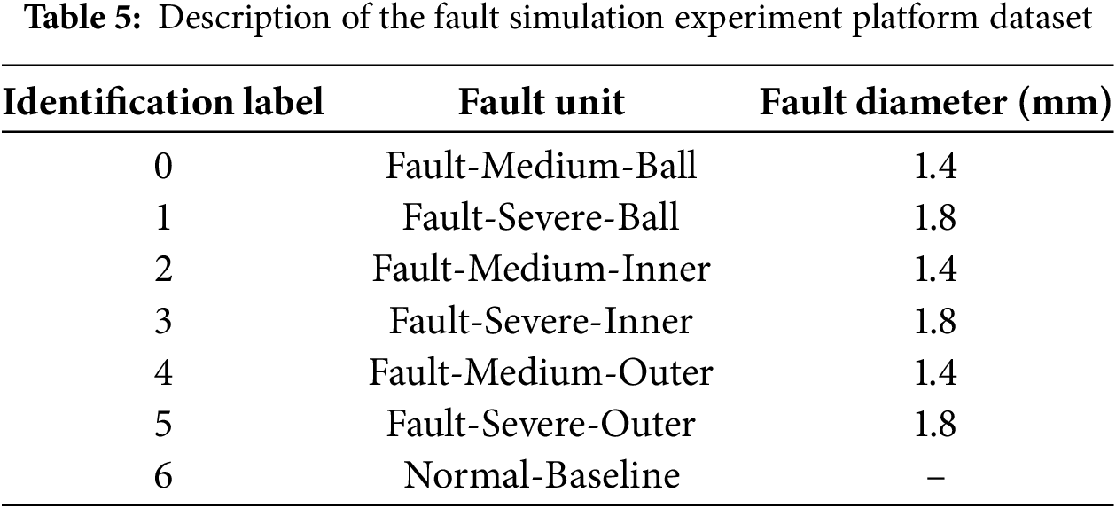
Under the 1 HP operating condition of the CWRU dataset, the experimental motor operated at a speed of 1772 rpm. Normal and fault data for the drive-end bearings were sampled at a frequency of 12 kHz. The CWRU dataset consists of four different fault categories: normal (N), outer ring fault (OR), inner ring fault (IR) and ball fault (B). Each fault category includes three different fault sizes: 0.007, 0.014, and 0.021 inches. Therefore, the experiment involved a total of 10 operating states in the CWRU dataset. The bearing fault simulation test platform was used to collect fault data under constant speed conditions. The experimental platform is principally constructed from an active motor, a radial loading device, and precision bearings, complemented by accelerometers for vibration monitoring, a laptop-based control interface, load motors with frequency converters, and an NI9234 data acquisition module. During the experiment, an accelerometer was positioned at the upper end of the bearing seat to collect vibration signals for analysis. The sampling frequency was set to 12.8 kHz, with a sampling duration of 15 s. The speed and load were maintained at 2400 rpm and 0.5 MPa, respectively. The bearing model used was N1006EM, with its physical parameters provided in Table 3. The processing of bearing rolling elements, along with inner and outer ring pitting faults, was carried out using electrical discharge machining. The fault diameters were set to 1.4 mm for moderate faults and 1.8 mm for severe faults. Therefore, the experiment involved a total of seven fault states. The specific classification and label definitions are provided in Tables 4 and 5, respectively.

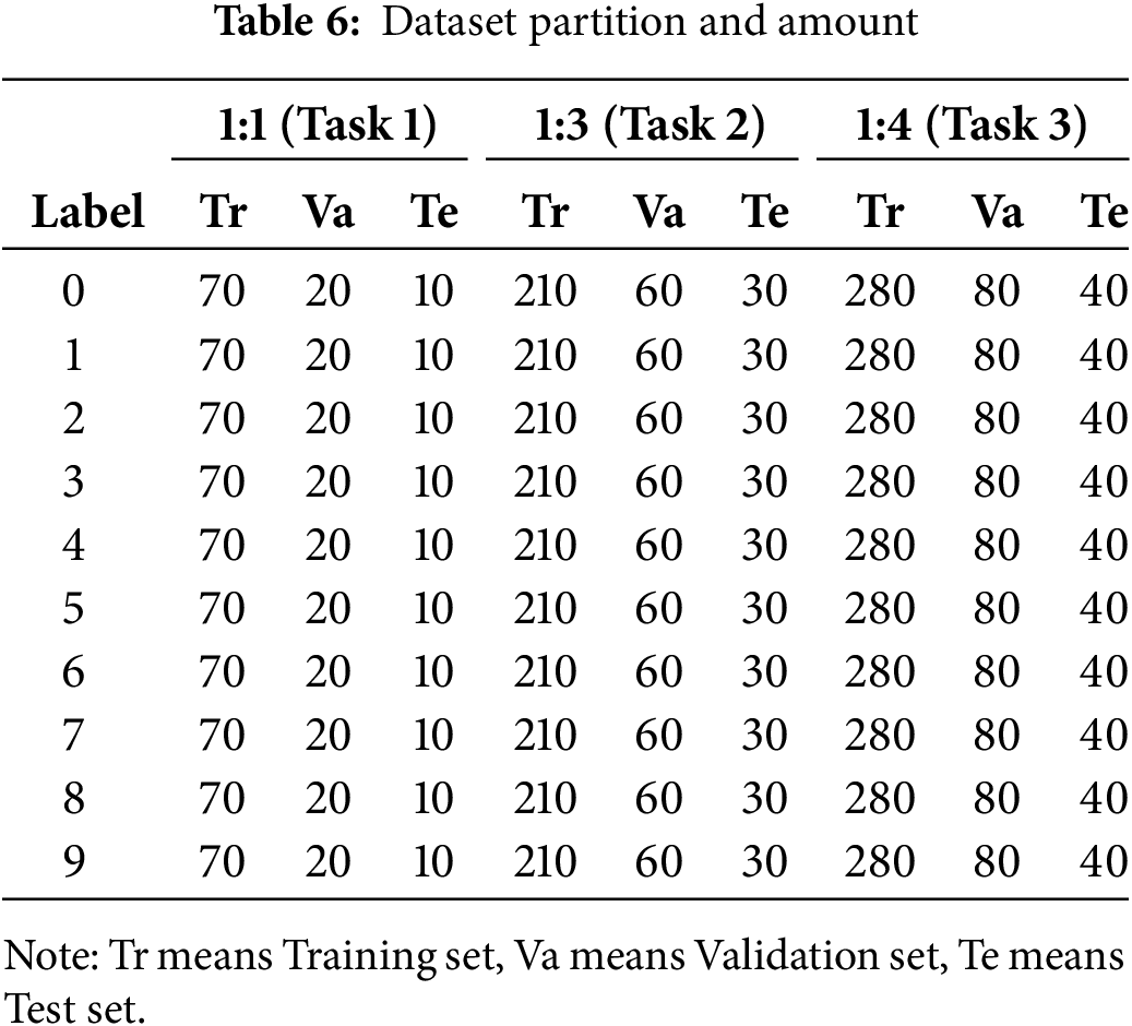
The original vibration signals of the experimental bearings in two datasets were segmented into independent samples containing 1024 data points under each different operating state, generating a total of 100 samples. Following signal normalization and the application of CWT and GIT for two-dimensional image conversion, 100 one-dimensional signal samples, grayscale images, and time-frequency graphs were obtained for each working condition. Consequently, the dataset was partitioned into training, validation, and test sets at a ratio of 7:2:1. Within the data augmentation module, three augmentation tasks were established for experimentation: no data augmentation, 1:3 ratio data augmentation, and a 1:4 ratio enhanced task involving a mixture of synthetic and original data. The primary objective of these tasks was to investigate the impact of varying data enhanced ratios on the diagnostic accuracy of the model. With the CWRU dataset taken as an example, detailed information regarding the dataset partitioning and the augmentation tasks is presented in Table 6.

4.2 Experiments with the CWRU Dataset

4.2.1 Data Quality Assessment and Analysis

Following the training of the 1DWDCGAN model for data synthesis, the time domain spectrum of real and synthetic samples were computed and compared across 10 fault conditions, as illustrated in Fig. 4. As shown in the figure, the synthetic samples exhibit considerable diversity across various fault conditions while retaining the essential characteristics of the original signals.

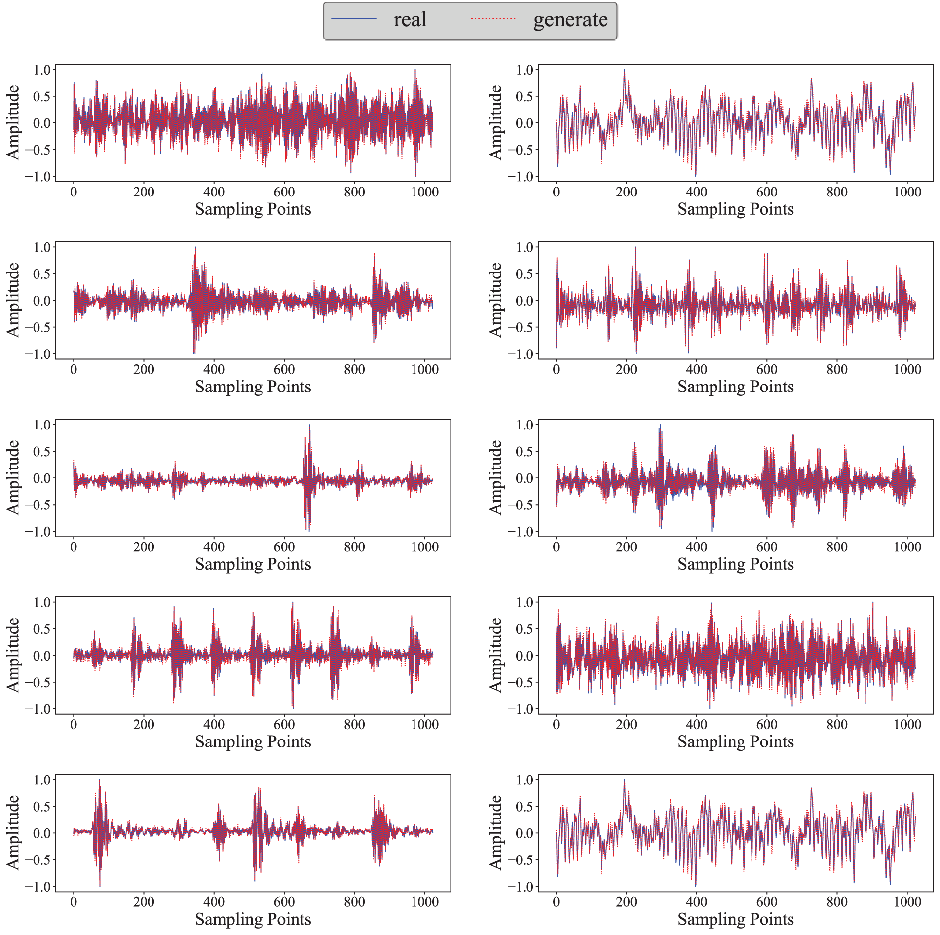
Figure 4: Comparison of the time domain waveform between real samples and generated samples

The quality of time-frequency and grayscale images directly influences the effectiveness of fault diagnosis. If the generated two-dimensional image samples accurately reflect the potential data distribution characteristics provided by real images, they may serve as a robust representational foundation for subsequent fault diagnosis models. The comparison between the real samples and the generated samples is presented in Figs. 5 and 6.

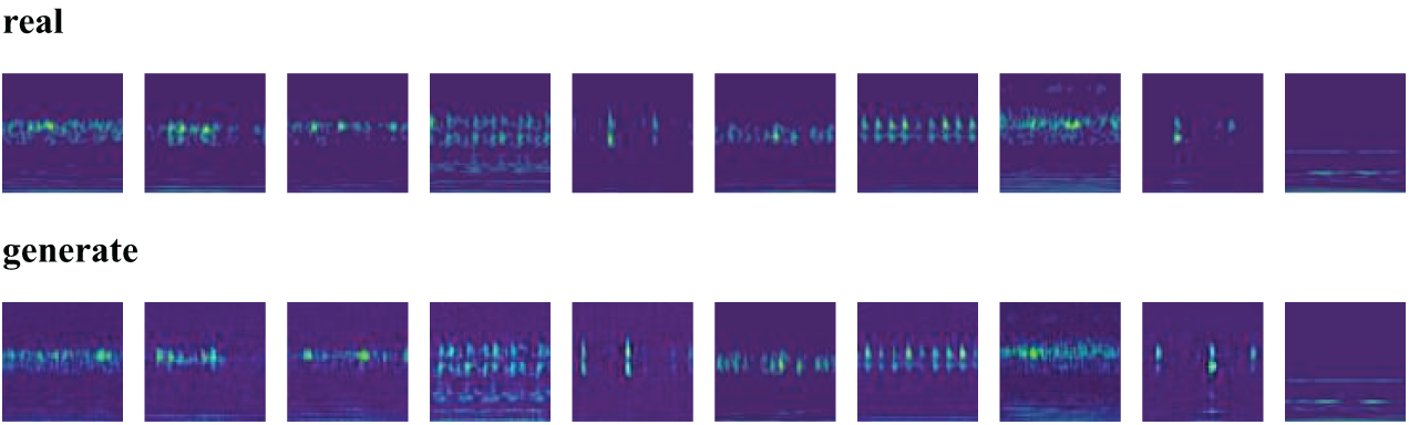
Figure 5: Comparison of the time-frequency images of real samples and generated samples

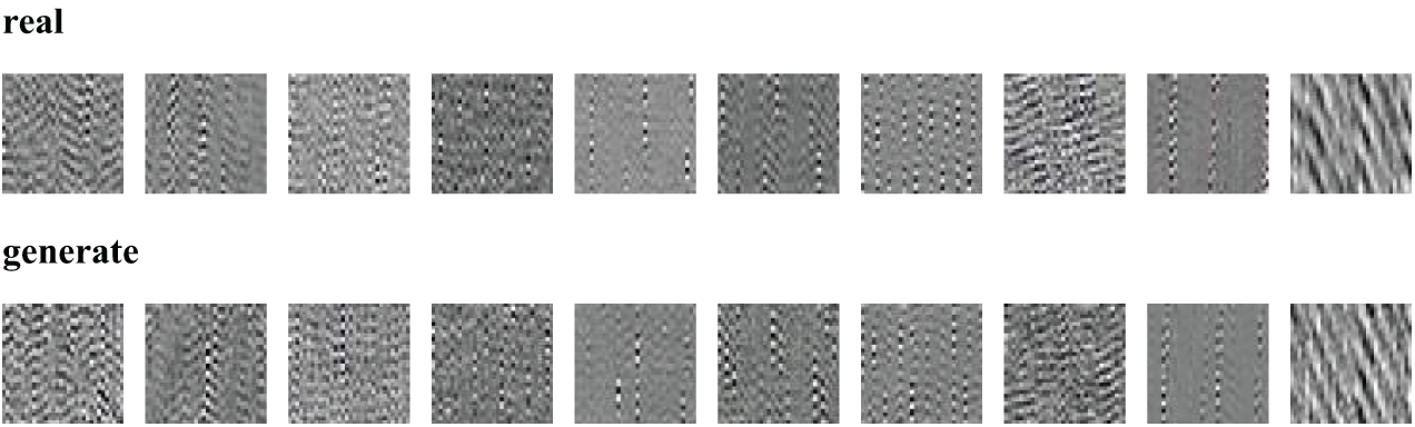
Figure 6: Comparison of the grayscale images of real samples and generated samples

A comparison between the generated images and the original images reveals that the features within the generated samples exhibit a distribution that is largely consistent with the features of the real samples. The tiny differences highlight the ability of the generative model to learn the distribution of the real data and its capacity to capture complex data distributions, rather than merely replicating the original samples. An arbitrary fault condition was selected to analyze quantitatively the differences in data distribution between the generated samples of the time-frequency images and grayscale images and their corresponding real samples. The pixel data were segmented into multiple intervals, and the frequency for each interval was computed to produce histograms that visualize the data distributions of both sets. Fig. 7a represents the data distribution of the time-frequency graphs, while Fig. 7b corresponds to that of the grayscale images. This demonstrates a high degree of congruence in feature distribution between the generated data and the real data while also showcasing the unique capability possessed by the generative model to produce diverse data. Therefore, the similarities observed between the synthesized data of the three types and the real data validate the effectiveness of the one-dimensional and two-dimensional WDCGAN model data augmentation framework utilized in this study within a multidimensional data space, effectively alleviating issues of inadequate data.

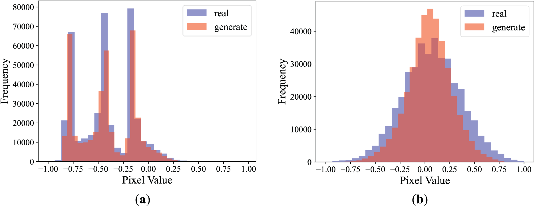
Figure 7: Comparison of real and generated data distribution: (a) the data distribution of the time-frequency graphs, (b) the data distribution of the grayscale images

The introduction of the SALTCT mechanism allows the WDCGAN model to adjust its training strategy flexibly when confronted with the challenges of different training stages, ensuring a balanced and stable training process for the generator and the discriminator, thereby mitigating the risk of overfitting due to excessive training of either component. The loss of the generator and discriminator of the standard model and the model after the introduction of the SALTCT mechanism are shown in Fig. 8, from which it can be observed that the optimization speeds of the generator loss and discriminator loss after the introduction of the SALTCT mechanism are better than those of the standard model. In addition, the loss curve of the improved model is more stable in the late stage of training, which indicates that the improved model has stronger robustness and stability in the face of complex data, while the fluctuation within a certain range indicates that the model is constantly optimized without local optimality, thus improving the training efficiency.

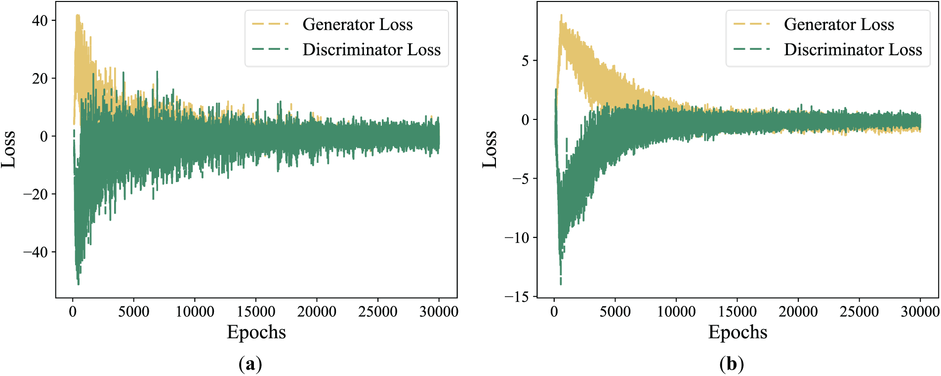
Figure 8: Loss of generator and discriminator: (a) Standard model, (b) Improved model

4.2.2 Results and Comparison of Small-Sample Fault Diagnosis

To illustrate further the of the proposed method in dealing with small-sample fault diagnosis with multidimensional information inputs, this study used one-dimensional and two-dimensional WDCGAN data augmentation models to set up the dataset with an augmentation ratio of 1:1 as a small-sample dataset according to different expansion ratios, as described in 4.1, and it was augmented with the data to construct a new dataset. The specific methods of using them to train different diagnostic models for diagnosis are shown in Table 7.

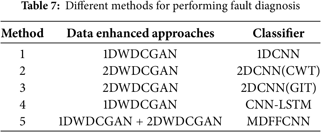
During the experimental process, the 1DCNN and 2DCNN network architectures and parameter settings employed in Methods 1, 2, and 3 were ensured to be identical to those proposed in Method 4 of this study. Each method was subjected to 10 tests to minimize random errors. The average testing results are illustrated in Table 8 and Fig. 9.

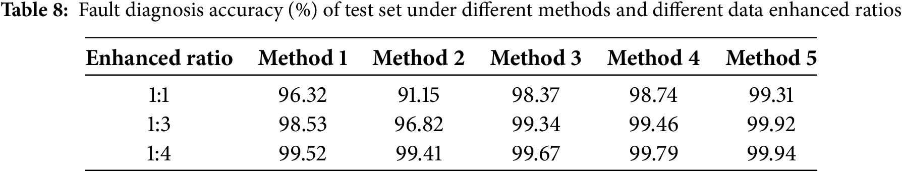
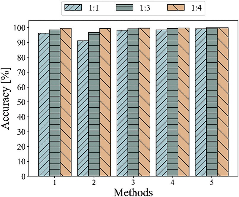
Figure 9: Classification accuracy of five methods with different data enhanced ratios

In Fig. 9, the x-axis represents the different experimental methods under the three data-enhanced ratios, and the y-axis represents the accuracy of classification. Table 6 shows that the classification accuracy of the proposed method is remarkably improved in diagnosis. In Task 1 without data enhancement, the diagnosis accuracy of MDFFCNN model proposed in this study reaches 99.31%. Compared with the other four comparison models, the accuracy rate is increased by 2.99%, 8.16%, 0.94%, and 0.57%. In addition, the confusion matrix can intuitively display the classification of various fault types, and predict labels can be obtained by inputting test set samples into the model for training. Therefore, the confusion matrix is introduced to evaluate the model and further verify its reliability. The confusion matrices of different methods are shown in Fig. 10.

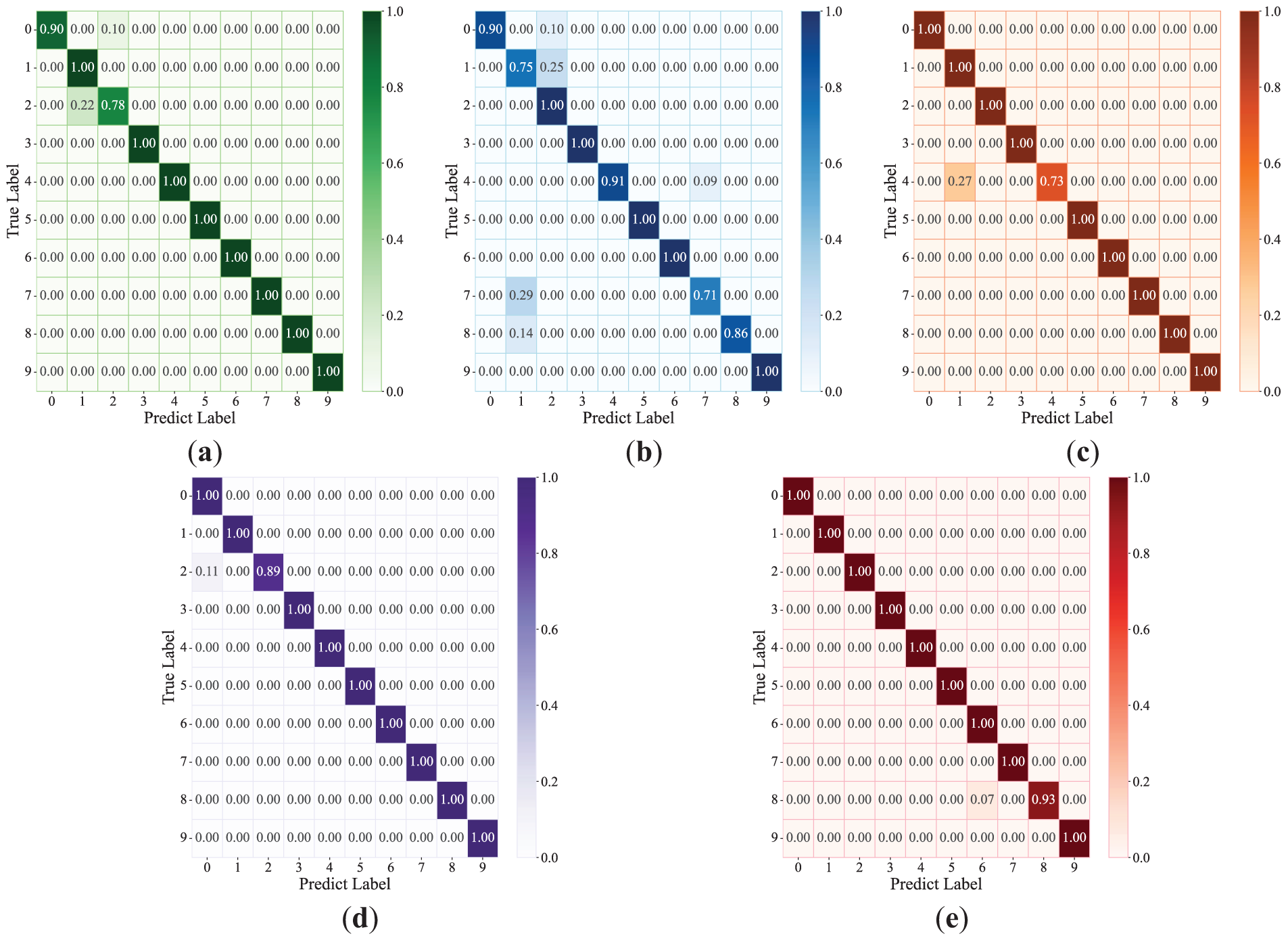
Figure 10: Comparison of confusion matrices for different diagnostic methods in Task 1: (a) Method 1, (b) Method 2, (c) Method 3, (d) Method 4, (e) Method 5

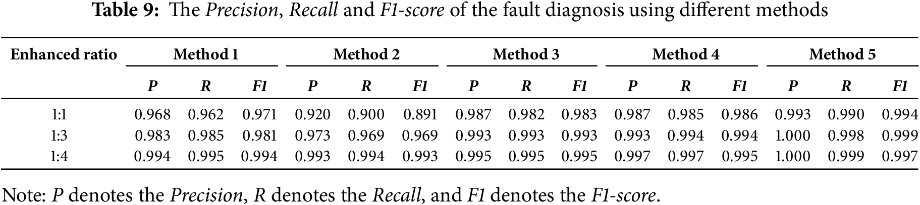
In Tasks 2 and 3 with different data-enhanced ratios, the accuracy of the test set on the MDFFCNN model reaches over 99.80% through sample expansion of the original dataset by 1DWDCGAN and 2DWDCGAN, which are improved in different degrees compared with other methods. However, reflecting the performance of the model fully by only relying on the accuracy rate as the evaluation index is often difficult. To reveal the performance of the model in the fault diagnosis task, this study selects Precision, Recall, and F1-score with more detailed and comprehensive evaluation capabilities as the additional evaluation indexes of the test to better reflect the predicted performance of the model. Precision directly measures the proportion of true positive samples among those identified as positive by the model; Recall can reflect the correct proportion of each type of fault; F1-score can reflect the comprehensive level of Precision and Recall. The higher the value is, the more accurate the model classification is. The calculation methods of the three are as follows [9]:

Precision=TPTP+FP,(13)

Recall=TPTP+FN,(14)

F1−score=2×Precision×RecallPrecision+Recall,(15)

where TP represents true positive case, TN represents true counterexample, FP represents false positive case, and FN represents false counterexample. The test results are shown in Table 9. In the experiment, the three prediction indicators of all methods under data enhancement are higher than the prediction results of the original dataset. With the increase in the data enhancement ratio, the failure dataset is supplemented; thus, the performance indicators, such as Precision, Recall, and F1-score, are improved synchronously. Therefore, the data enhancement model used in this study can effectively solve the inadequate data phenomenon, provide sufficient data basis for the follow-up diagnosis model training, and improve the diagnosis accuracy and efficiency.

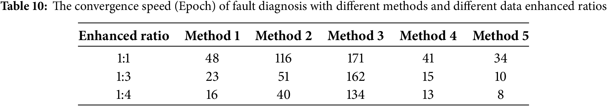
The proposed method in this study has shown remarkable advantages in many aspects, not only surpassing the single-dimensional detection method enhanced on the basis of different proportions of data on the quantitative index of prediction performance but also achieving increased convergence rate in the model training stage, which marks the dual optimization of the method in improving the detection efficiency and accuracy. In this study, a function is defined to judge whether the model is stable and converged. When the fluctuation of the accuracy of the verification set is less than Q in the continuous N iterations of the model, the model is considered to be stable and converged. In this process, N was set to 4, and Q was established at 0.005. The number of iterations for the dataset to achieve stable convergence during training under two operating conditions is shown in Table 10. As shown in the table, the proposed method reached convergence at the 34th iteration during training on the dataset without data augmentation under different operating conditions. In training under different data augmentation ratios, the proposed model can reach convergence within 10 iterations. Compared with other fault diagnosis methods, the method in this study not only has increased convergence speed but also can effectively relieve the inadequate data problem through data enhancement technology while guaranteeing diagnosis accuracy and enhance the generalization capacity and robustness of the model, thus showing stronger adaptability and reliability in the actual application.

4.3 Experiments with the Fault Simulation Experimental Platform Dataset

4.3.1 Stability Analysis of the Model Training Process

In the experiments with the fault simulation experimental platform dataset, the variation of the generator and discriminator losses in five different network architectures, including the proposed method, is compared, as shown in Fig. 11. The experimental results show that although all the methods exhibit a certain degree of loss fluctuation during the training process, the fluctuation amplitude of the loss curve for the method proposed in this study is considerably lower than that of the other comparison methods, and the training process is overall more stable. Furthermore, the proposed method achieves the lowest final loss values, further highlighting its superior performance. This phenomenon indicates that SALTCT can effectively suppress the instability in the training process, avoid the risk of overtraining of generators and discriminators, and improve the convergence and robustness of the model. The stability of the loss curve also reflects that the method has stronger adaptability to complex datasets and can be continuously optimized without converging to a local optimum.

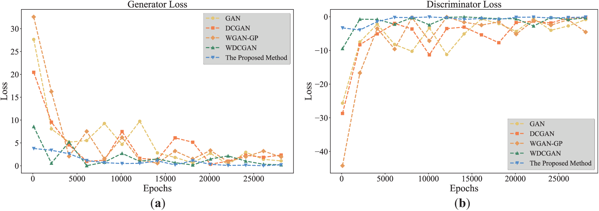
Figure 11: Comparison of generator and discriminator loss curves with different methods: (a) Generator loss, (b) Discriminator loss

4.3.2 Results and Comparison of Small-Sample Fault Diagnosis

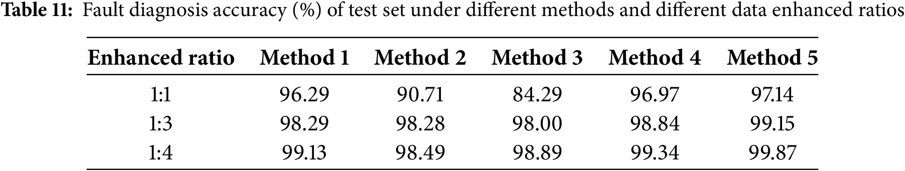
In the process of implementing small-sample fault diagnosis, training tests are conducted in accordance with the new datasets of different data enhancement tasks as the input of the diagnosis model. Fig. 12 and Table 11 show the fault diagnosis accuracy comparison of different methods under different data enhancement ratios. Method 3 showed poor diagnostic accuracy in Task 1 of small sample without data enhancement, which may be related to its insufficient adaptability in different experimental environments and operating conditions. The diagnostic results after sample expansion of Tasks 2 and 3 showed a high accuracy rate of over 98%, thus verifying the influence of sample size on diagnostic accuracy. The accuracy rate of the proposed method reaches 99.87% under the mission with the enhancement ratio of 1:4, and the accuracy rate increases by 0.74%, 1.38%, 0.98%, and 0.53% compared with other methods. In addition, the diagnosis accuracy under the other two tasks is improved to different degrees compared with other methods, which verifies the remarkable advantages of this method in fault diagnosis under the background of data scarcity and the generalization ability and strong robustness of this method in a complex and changeable experimental environment.

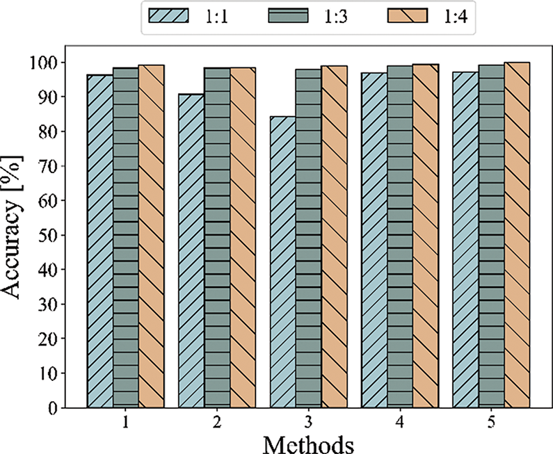
Figure 12: Classification accuracy of five methods with different data enhanced ratios

On the basis of Accuracy, Precision, Recall, and F1-score, the ROC-AUC is introduced in this study as a metric for evaluating model performance. The ROC curve can illustrate the model’s performance across different thresholds, enabling a comprehensive understanding of the trade-off between sensitivity and specificity, which is crucial to addressing the requirements of various application scenarios. ROC-AUC is a standardized metric that allows for the comparison of model performance on the same task, regardless of the specific implementation or parameter settings, thereby facilitating a comparative evaluation of the performance of different models. Fig. 13 presents the ROC curves for each model in Task 1 and the quantitative AUC metrics for the ROC curves. As the apex of the ROC curve approaches the upper-left corner, the discriminatory power of the model increases, with increased sensitivity and specificity. Therefore, Fig. 13 indicates that the AUC value of the proposed method reaches 0.9946, which is improved in different degrees compared with other models; thus, it is more sensitive and reliable.

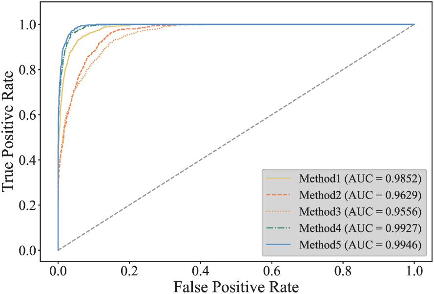
Figure 13: ROC curve and AUC for each method

In practical industrial settings, the raw signals collected by sensors often contain considerable background noise. Gaussian white noise of varying intensities is added to the original signals to assess the robustness of the model under strong background noise. Signal-to-noise ratio (SNR) is employed as an indicator of noise magnitude, and its definition is described as follows:

SNR=10log10⁡PsPn,(16)

where Ps denotes the signal power, and Pn denotes the noise power. When the SNR is below 0, it indicates that the noise energy exceeds that of the original signal, making it challenging to extract meaningful features from the noisy signal. In the SNR range of −2–6 dB, diagnostic accuracy tests were conducted 10 times under different noise conditions for each method, and the average values were calculated, as shown in Fig. 14. As shown in the figure, at SNR values of −2 and 0, the accuracy of the proposed method is 75.62% and 82.33%, respectively, demonstrating a similar poor performance as the other methods. This result suggests that these models are not suitable for fault diagnosis in environments with strong noise backgrounds. However, as the SNR increases, diagnostic accuracy improves, reaching over 90% at SNR = 6, thereby confirming the robustness of the proposed method in various noise conditions.

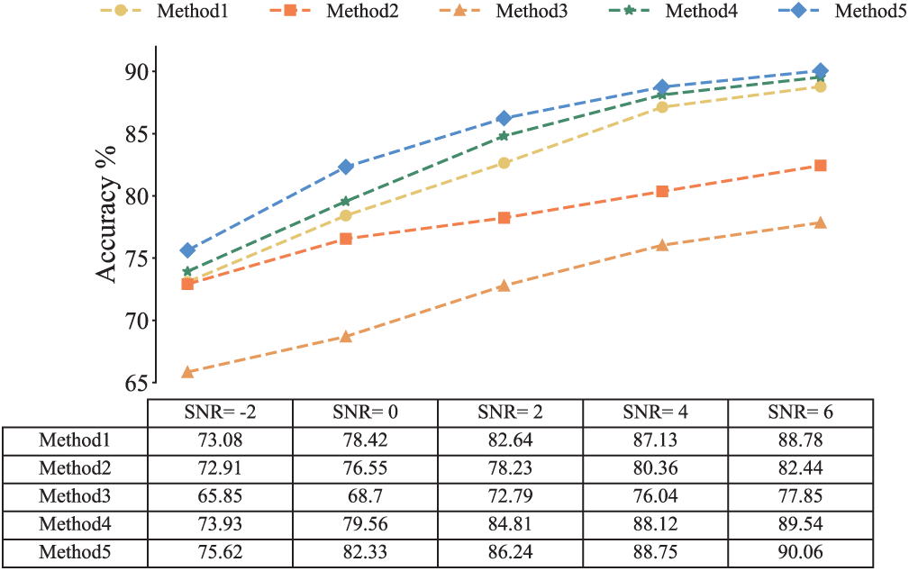
Figure 14: The accuracy of different methods under different noise environment

4.4 Timeliness of Fault Diagnosis

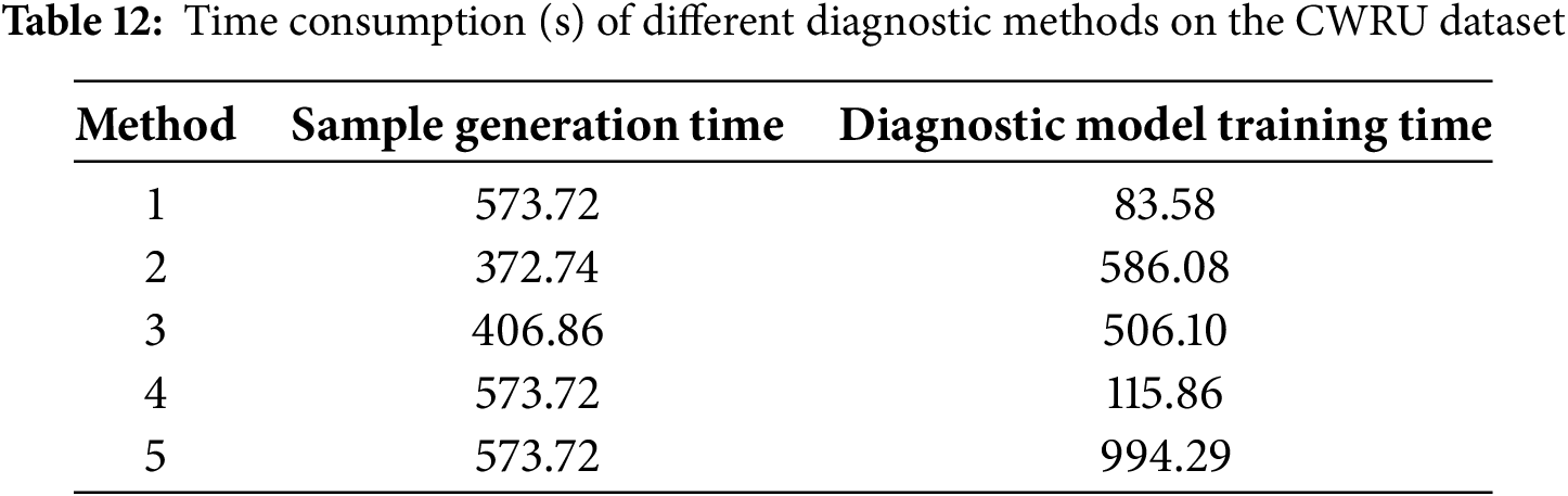
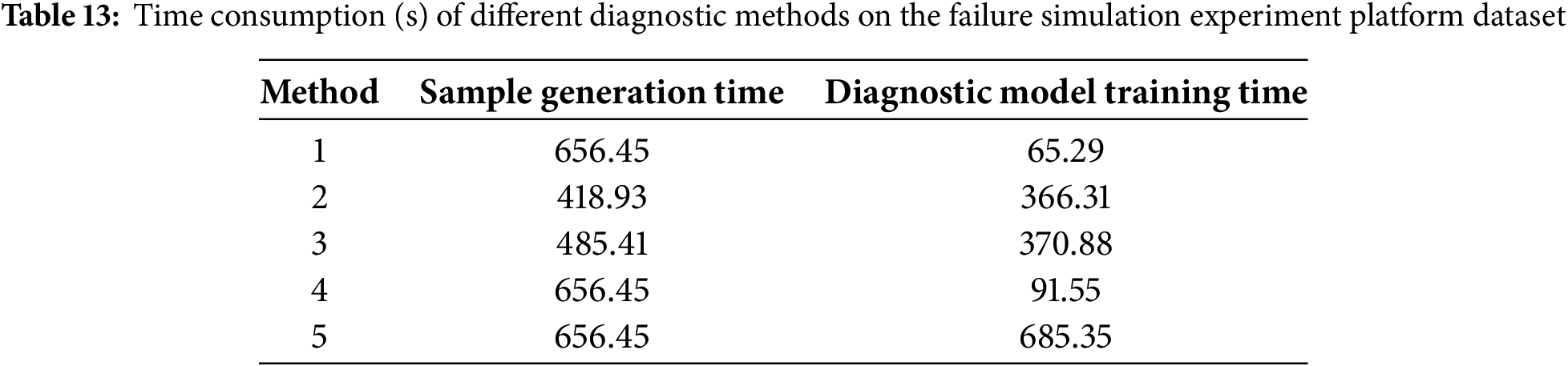
To demonstrate further the timeliness of the fault diagnosis method proposed in this article, Tables 12 and 13 respectively calculate the sample generation time and diagnostic model training time for the two datasets under the enhanced ratio of 1:4 task. As shown in the table, the main time consumption among all methods is the generation of samples. In terms of diagnostic model time consumption, the method proposed in this study takes the longest time because to improve diagnostic accuracy, three different features are fused, and the large number of model parameters leads to a long training time. In consideration of the diagnostic accuracy and robustness of the diagnostic model, the method proposed in this study can achieve good diagnostic results with little impact on time consumption. The environment of the whole experiment is as follows: CPU, Intel Corei5-13400F; GPU, NVIDIA RTX 4060 and Python 3.9.

5  Conclusion

A novel diagnosis method for rolling bearing under a small-sample condition is proposed in this study. This method leverages an original dataset to generate new samples in multiple dimensions through improved 1D-2DWDCGAN dual models, thereby expanding the dataset. Subsequently, multidimensional feature fusion and detection are performed on the compensated dataset using the MDFFCNN model. Experimental validation is conducted on a bearing dataset under various operating conditions. Results illustrate that the proposed 1D-2DWDCGAN dual models validate its capability to generate high-quality samples by comparing the similarity between generated samples and actual samples and achieving data enhancement. Concurrently, the self-adaptive loss threshold control strategy further refines the parameter adjustments during the training process, enabling the model to converge more stably toward the optimal solution, thereby accelerating training speed. Finally, the fault diagnosis method based on the MDFFCNN utilizes a multilayer convolutional network structure that automatically learns and extracts deep features from raw data, integrating multidimensional features such as waveform features, structured features, and time-frequency features to form composite deep features. In comparisons of multiple diagnostic methods under varying data enhanced ratios, the proposed model demonstrates remarkable improvements in quantifiable metrics and convergence speed, with the enhancement effect becoming more pronounced as the enhancement ratio increases, thereby fully leveraging the complementarity among different dimensional information to achieve high-precision fault diagnosis.

Although the proposed method has achieved satisfactory results in the diagnosis of small-sample faults, several areas warrant further exploration, e.g., the optimization and improvement of the data generation model architecture and the investigation of strategies to reduce the computational costs of the overall workflow. While these works may be associated with an increase in computational load, they are still worthy of investigation due to their potential contribution to enhancing diagnostic accuracy.

Acknowledgement: Not applicable.

Funding Statement: This work was supported by the National Natural Science Foundation of China (Grant Nos. 12272259 and 52005148).

Author Contributions: The authors confirm contribution to the paper as follows: study conception and design: Qiang Ma, Zhuopei Wei, Kai Yang; data collection: Qiang Ma, Kai Yang; analysis and interpretation of results: Zhuopei Wei, Kai Yang; draft manuscript preparation: Zhuopei Wei, Long Tian, Zepeng Li. All authors reviewed the results and approved the final version of the manuscript.

Availability of Data and Materials: The authors confirm that the data supporting the findings of this study are available within the article.

Ethics Approval: Not applicable.

Conflicts of Interest: The authors declare no conflicts of interest to report regarding the present study.

References

1. Zhang J, Yi S, Guo L, Gao H, Hong X, Song H. A new bearing fault diagnosis method based on modified convolutional neural networks. Chin J Aeronaut. 2020;33(2):439–47. doi:10.1016/j.cja.2019.07.011. [Google Scholar] [CrossRef]

2. Wang R, Jiang H, Zhu K, Wang Y, Liu C. A deep feature enhanced reinforcement learning method for rolling bearing fault diagnosis. Adv Eng Inform. 2022;54:101750. doi:10.1016/j.aei.2022.101750. [Google Scholar] [CrossRef]

3. Ma J, Shang J, Zhao X, Zhong P. Bayes-DCGRU with Bayesian optimization for rolling bearing fault diagnosis. Appl Intell. 2022;52(10):11172–83. doi:10.1007/s10489-021-02924-z. [Google Scholar] [CrossRef]

4. Ni Q, Ji JC, Halkon B, Feng K, Nandi AK. Physics-informed residual network (PIResNet) for rolling element bearing fault diagnostics. Mech Syst Signal Process. 2023;200:110544. doi:10.1016/j.ymssp.2023.110544. [Google Scholar] [CrossRef]

5. Hou W, Zhang C, Jiang Y, Cai K, Wang Y, Li N. A new bearing fault diagnosis method via simulation data driving transfer learning without target fault data. Measurement. 2023;215:112879. doi:10.1016/j.measurement.2023.112879. [Google Scholar] [CrossRef]

6. Chauhan S, Vashishtha G, Zimroz R, Kumar R, Gupta MK. Optimal filter design using mountain gazelle optimizer driven by novel sparsity index and its application to fault diagnosis. Appl Acoust. 2024;225:110200. doi:10.1016/j.apacoust.2024.110200. [Google Scholar] [CrossRef]

7. Cheng Y, Tian Z, Ning D, Feng K, Li Z, Chauhan S, et al. Computer vision-based non-contact structural vibration measurement: methods, challenges and opportunities. Measurement. 2024;243:116426. doi:10.1016/j.measurement.2024.116426. [Google Scholar] [CrossRef]

8. Liu Y, Jiang H, Liu C, Yang W, Sun W. Data-augmented wavelet capsule generative adversarial network for rolling bearing fault diagnosis. Knowl-Based Syst. 2022;252:109439. doi:10.1016/j.knosys.2022.109439. [Google Scholar] [CrossRef]

9. Zhou F, Yang S, Fujita H, Chen D, Wen C. Deep learning fault diagnosis method based on global optimization GAN for unbalanced data. Knowl-Based Syst. 2020;187:104837. doi:10.1016/j.knosys.2019.07.008. [Google Scholar] [CrossRef]

10. Shao S, Wang P, Yan R. Generative adversarial networks for data augmentation in machine fault diagnosis. Comput Ind. 2019;106:85–93. doi:10.1016/j.compind.2019.01.001. [Google Scholar] [CrossRef]

11. Liu J, Zhang C, Jiang X. Imbalanced fault diagnosis of rolling bearing using improved MsR-GAN and feature enhancement-driven CapsNet. Mech Syst Signal Process. 2022;168:108664. doi:10.1016/j.ymssp.2021.108664. [Google Scholar] [CrossRef]

12. Zhang T, Chen J, Li F, Zhang K, Lv H, He S, et al. Intelligent fault diagnosis of machines with small & imbalanced data: a state-of-the-art review and possible extensions. ISA Trans. 2022;119:152–71. doi:10.1016/j.isatra.2021.02.042. [Google Scholar] [PubMed] [CrossRef]

13. Pan T, Chen J, Zhang T, Liu S, He S, Lv H. Generative adversarial network in mechanical fault diagnosis under small sample: a systematic review on applications and future perspectives. ISA Trans. 2022;128:1–10. doi:10.1016/j.isatra.2021.11.040. [Google Scholar] [PubMed] [CrossRef]

14. Li R, Li S, Xu K, Zeng M, Li X, Gu J, et al. Auxiliary generative mutual adversarial networks for class-imbalanced fault diagnosis under small samples. Chin J Aeronaut. 2023;36(9):464–78. doi:10.1016/j.cja.2022.12.015. [Google Scholar] [CrossRef]

15. Zhao H, Yang X, Chen B, Chen H, Deng W. Bearing fault diagnosis using transfer learning and optimized deep belief network. Meas Sci Technol. 2022;33(6):065009. doi:10.1088/1361-6501/ac543a. [Google Scholar] [CrossRef]

16. Chen J, Huang R, Chen Z, Mao W, Li W. Transfer learning algorithms for bearing remaining useful life prediction: a comprehensive review from an industrial application perspective. Mech Syst Signal Process. 2023;193:110239. doi:10.1016/j.ymssp.2023.110239. [Google Scholar] [CrossRef]

17. Ding Y, Jia M, Zhuang J, Cao Y, Zhao X, Lee C. Deep imbalanced domain adaptation for transfer learning fault diagnosis of bearings under multiple working conditions. Reliab Eng Syst Saf. 2023;230:108890. doi:10.1016/j.ress.2022.108890. [Google Scholar] [CrossRef]

18. Qian Q, Qin Y, Luo J, Wang Y, Wu F. Deep discriminative transfer learning network for cross-machine fault diagnosis. Mech Syst Signal Process. 2023;186:109884. doi:10.1016/j.ymssp.2022.109884. [Google Scholar] [CrossRef]

19. Huisman M, Plaat A, van Rijn JN. Understanding transfer learning and gradient-based meta-learning techniques. Mach Learn. 2024;113(7):4113–32. doi:10.1007/s10994-023-06387-w. [Google Scholar] [CrossRef]

20. Li C, Li S, Zhang A, He Q, Liao Z, Hu J. Meta-learning for few-shot bearing fault diagnosis under complex working conditions. Neurocomputing. 2021;439:197–211. doi:10.1016/j.neucom.2021.01.099. [Google Scholar] [CrossRef]

21. Chang L, Lin YH. Meta-learning with adaptive learning rates for few-shot fault diagnosis. IEEE/ASME Trans Mechatron. 2022;27(6):5948–58. doi:10.1109/TMECH.2022.3192122. [Google Scholar] [CrossRef]

22. Chawla NV, Bowyer KW, Hall LO, Kegelmeyer WP. SMOTE: synthetic minority over-sampling technique. J Artif Intell Res. 2002;16:321–57. doi:10.1613/jair.953. [Google Scholar] [CrossRef]

23. Goodfellow I, Pouget-Abadie J, Mirza M, Xu B, Warde-Farley D, Ozair S, et al. Generative adversarial nets. Adv Neural Inf Process Syst. 2014;27:1–9. [Google Scholar]

24. Radford A, Metz L, Chintala S. Unsupervised representation learning with deep convolutional generative adversarial networks. arXiv:1511.06434. 2015. [Google Scholar]

25. Li J, Chen Z, Cheng L, Liu X. Energy data generation with Wasserstein deep convolutional generative adversarial networks. Energy. 2022;257:124694. doi:10.1016/j.energy.2022.124694. [Google Scholar] [CrossRef]

26. Guo Y, Zhou Y, Zhang Z. Fault diagnosis of multi-channel data by the CNN with the multilinear principal component analysis. Measurement. 2021;171:108513. doi:10.1016/j.measurement.2020.108513. [Google Scholar] [CrossRef]

27. He Z, Shao H, Zhong X, Zhao X. Ensemble transfer CNNs driven by multi-channel signals for fault diagnosis of rotating machinery across working conditions. Knowl-Based Syst. 2020;207:106396. doi:10.1016/j.knosys.2020.106396. [Google Scholar] [CrossRef]

28. Ruan D, Wang J, Yan J, Gühmann C. CNN parameter design based on fault signal analysis and its application in bearing fault diagnosis. Adv Eng Inform. 2023;55:101877. doi:10.1016/j.aei.2023.101877. [Google Scholar] [CrossRef]

29. Zhao K, Xiao J, Li C, Xu Z, Yue M. Fault diagnosis of rolling bearing using CNN and PCA fractal based feature extraction. Measurement. 2023;223:113754. doi:10.1016/j.measurement.2023.113754. [Google Scholar] [CrossRef]

30. Zhong S, Fu S, Lin L. A novel gas turbine fault diagnosis method based on transfer learning with CNN. Measurement. 2019;137:435–53. doi:10.1016/j.measurement.2019.01.022. [Google Scholar] [CrossRef]

31. Huang T, Zhang Q, Tang X, Zhao S, Lu X. A novel fault diagnosis method based on CNN and LSTM and its application in fault diagnosis for complex systems. Artif Intell Rev. 2022;55(2):1289–315. doi:10.1007/s10462-021-09993-z. [Google Scholar] [CrossRef]

32. Chen R, Huang X, Yang L, Xu X, Zhang X, Zhang Y. Intelligent fault diagnosis method of planetary gearboxes based on convolutional neural network and discrete wavelet transform. Comput Ind. 2019;106:48–59. doi:10.1016/j.compind.2018.11.003. [Google Scholar] [CrossRef]

33. Gao S, Jiang Z, Liu S. An approach to intelligent fault diagnosis of cryocooler using time-frequency image and CNN. Comput Intell Neurosci. 2022;1:1754726. doi:10.1155/2022/1754726. [Google Scholar] [PubMed] [CrossRef]

34. Zhang C, Yu J, Wang S. Fault detection and recognition of multivariate process based on feature learning of one-dimensional convolutional neural network and stacked denoised autoencoder. Int J Prod Res. 2021;59(8):2426–49. doi:10.1080/00207543.2020.1733701. [Google Scholar] [CrossRef]

35. Ye M, Yan X, Chen N, Jia M. Intelligent fault diagnosis of rolling bearing using variational mode extraction and improved one-dimensional convolutional neural network. Appl Acoust. 2023;202:109143. doi:10.1016/j.apacoust.2022.109143. [Google Scholar] [CrossRef]

36. Qin Y, Shi X. Fault diagnosis method for rolling bearings based on two-channel CNN under unbalanced datasets. Appl Sci. 2022;12(17):8474. doi:10.3390/app12178474. [Google Scholar] [CrossRef]

37. Arjovsky M, Chintala S, Bottou L. Wasserstein generative adversarial networks. In: Proceedings of the 34th International Conference on Machine Learning; 2017; Sydney, Australia. Vol. 70, p. 214–23. [Google Scholar]

38. Gulrajani I, Ahmed F, Arjovsky M, Dumoulin V, Courville AC. Improved training of Wasserstein GANs. Adv Neural Inf Process Syst. 2017;30:1–11. [Google Scholar]

39. Chen J, Yan Z, Lin C, Yao B, Ge H. Aero-engine high speed bearing fault diagnosis for data imbalance: a sample enhanced diagnostic method based on pre-training WGAN-GP. Measurement. 2023;213:112709. doi:10.1016/j.measurement.2023.112709. [Google Scholar] [CrossRef]

40. Diao N, Wang Z, Ma H, Yang W. Fault diagnosis of rolling bearing under variable working conditions based on CWT and T-ResNet. J Vib Eng Technol. 2023;11(8):3747–57. doi:10.1007/s42417-022-00780-w. [Google Scholar] [CrossRef]

41. Fouladi R, Ermis O, Anarim E. A novel approach for distributed denial of service defense using continuous wavelet transform and convolutional neural network for software-defined network. Comput Secur. 2022;112:102524. doi:10.1016/j.cose.2021.102524. [Google Scholar] [CrossRef]

42. Chong UP. Signal model-based fault detection and diagnosis for induction motors using features of vibration signal in two-dimension domain. Stroj Vestn. 2011;57(9):655–66. doi:10.5545/sv-jme.2010.162. [Google Scholar] [CrossRef]

43. Case Western Reserve University. [cited 2024 Oct 12]. Available from: http://www.eecs.cwru.edu/laboratory/bearings/. [Google Scholar]