A Multi-Sensor and PCSV Asymptotic Classification Method for Additive Manufacturing High Precision and Efficient Fault Diagnosis

1  Introduction

Additive Manufacturing (AM), also known as 3D printing, integrates computer-aided design, material processing, and shaping technologies. It relies on digital model files to manufacture solid components by layering specialized metal, non-metal, and biomedical materials through methods such as extrusion, sintering, melting, light curing, and jetting [1,2]. On the one hand, as one of the advanced manufacturing industries, additive manufacturing is a set of “material-process-equipment” [3]. Materials and processes [4] directly affect the performance of processed parts. The stability of the equipment will also affect the efficiency of production. On the other hand, additive manufacturing equipment is highly integrated, and each module has its own fault diagnosis system. However, as the individual modules are highly interacted with each other [5,6], a single subsystem diagnosis is one-sided. Therefore, the multi-module fault diagnosis of additive manufacturing equipment is very necessary.

Multi-module fault diagnosis [7,8], as a crucial part of improving system reliability and safety, ensures the secure operation of the system and is important for preventing catastrophic accidents [9,10]. In recent years, Fault diagnosis has usually been classified into mathematical model-based and data-driven approaches. The former approach describes the state of fault occurrence through a mathematical model established by studying the fault mechanism [11]. However, for some complex mechanical systems, it is very difficult to establish complex mathematical models and accurately diagnose the causes of faults [12,13]. With the development of sensor technology and data analysis technology, data-driven approaches have received widespread attention for their ability to avoid the limitations of the complexity of the research object. Some data-driven methods determine whether a fault has occurred at the current moment by building statistical models of historical data. The integration of multiple data-driven models plays a crucial role in fault diagnosis by combining the strengths of different approaches to detect faults in complex systems more accurately and robustly. By fusing data from different models, the diagnostic process can utilize complementary information to improve the overall reliability and effectiveness of fault detection while reducing the likelihood of false alarms and missed diagnoses. In the industrial sector, the failure rate of industrial equipment is between 1% and 5%, resulting in the proportion of normal process data far exceeding the abnormal data. Therefore, a large amount of redundant data is generated, which affects the accuracy rate, training time, and decision time of the model [14]. To address the problem of data redundancy, Xue et al. [15] used principal component analysis (PCA) to characterize the conductivity data and remove the redundant background information, which further improves the data quality and reduces the computational burden. Fan et al. [16] based on PCA and minimum redundancy correlation analysis (MRCA) to achieve the performance monitoring and management of the drilling process. The proposed method is compared with slow feature analysis (SFA) [17] and distributed canonical variate analysis (D-CVA) [18] through three performance indicators: Non-detection rate (NDR), False alarm rate (FAR), and running time, the results demonstrate the superiority of PCA model in de-redundancy. Data-driven equipment fault diagnosis [19], which does not rely on the mechanism of fault generation, can classify monitoring data through machine learning or deep learning methods without prior knowledge, achieving state recognition [20,21]. Three key metrics for evaluating online fault diagnostic models are diagnostic accuracy, model training time, and model inference time. Rauber et al. [22] extracted the original feature vector containing 26 statistical parameters, 72 envelope features, and 32 wavelet packet features. Then SVM is used to recognize the bearing faults, and the fault diagnosis accuracy reached 98.1%. Guo et al. [23] proposed an intelligent time-varying adaptive data-driven approach to identify offset faults, stuck-at faults, and noise faults by using fault data such as phase currents, DC (Direct Current) link voltages, and rotational speed signals as inputs to the model, with an average diagnostic accuracy of 98%, and an average decision-making time of 10 ms after the occurrence of a fault. A novel hyperbolic fuzzy entropy method, which has a maximum accuracy of 97% [24]. It divides fault diagnosis into two steps, the first step identifies the defects, and depending on the type of faults, appropriate clustering techniques are used in the second step. Yang et al. [25] transformed the satellite attitude control system thruster fault diagnosis problem into a binary image classification problem and realized the online detection, diagnosis, and localization of thruster stuck-open and stuck-closed faults. The average accuracy is 98.54% without considering the decision time. Chine et al. [26] calculated several characteristic parameters and used the ANN (Artificial Neural Network) method to diagnose the faults of PV (photovoltaic) systems with a diagnostic accuracy of 90.7%.

The above methods rely on extensive fault samples for multi-classification fault diagnosis. However, in the industrial sector, fault samples are often insufficient, resulting in the proportion of normal process data far exceeding abnormal data. This imbalance leads to a large amount of redundant data, negatively impacting the model’s accuracy, training time, and decision-making time. Furthermore, while multi-classification models are designed for complex fault diagnosis, they are less efficient and accurate compared to binary classification models, particularly when dealing with limited data. To address these challenges, a PCSV asymptotic classification fault diagnosis method is proposed. Asymptotic Classification refers to a hierarchical, stage-wise classification methodology designed to address challenges in imbalanced and limited-data scenarios. It combines the efficiency of binary classification with the granularity of multi-class classification by progressively narrowing down the diagnostic process. Initially, a binary classifier rapidly distinguishes between normal and abnormal states to filter out redundant normal data, reducing computational overhead. Subsequently, only identified abnormal samples undergo finer-grained multi-classification to pinpoint specific fault types. The advantages of the proposed PCSV method can significantly reduce computational complexity, especially in large-scale industrial systems, through its efficient hierarchical approach. Additionally, focusing on abnormal samples for multi-class classification, improves diagnostic accuracy even in imbalanced and limited data scenarios, ensuring more reliable fault identification. Additionally, the study integrates advanced sensor technology to ensure reliable data acquisition, which is critical for accurate fault detection and classification. The main contributions of this study are as follows:

(1)   Adaptive feature selection mechanism: The proposed PCSV asymptotic classification method introduces an adaptive feature selection mechanism that dynamically identifies and prioritizes the most relevant features for each stage of fault diagnosis. By reducing redundancy and focusing only on the essential data, this mechanism improves the model’s efficiency and accuracy while minimizing the impact of imbalanced datasets. The feature selection is guided by a combination of statistical analysis and domain-specific heuristics, ensuring robustness across different industrial applications.

(2)   Aimed at additive manufacturing equipment, the research mainly focuses on the abnormal diagnosis of equipment parameters during the additive manufacturing process about analog and Boolean data (non-image data), including temperature, flow, pressure, and so on. A hierarchical decision-making framework is incorporated into the PCSV method, enabling a progressive refinement of fault classification. The framework begins with binary classifications to distinguish normal from abnormal states, followed by a multi-classification stage to diagnose specific faults. This tiered approach not only reduces computational complexity but also enhances the overall decision-making speed and reliability. The framework leverages a feedback mechanism to iteratively improve the model by incorporating new fault data, ensuring continuous learning and adaptability to evolving industrial environments.

The rest of the proposed research work is briefed as follows. Section 2 introduces the theoretical background of PCSV asymptotic classification, and analyzes and summarizes the metal additive manufacturing equipment fault mechanism analysis. Section 3 introduces PCSV asymptotic classification methods in metal additive manufacturing equipment. Section 4 describes the experimental process and data analysis in detail, including the experimental operation steps and data analysis methods. Finally, Section 5 summarizes the main conclusions and contributions of this study, and provides a prospect for future research directions.

2  Theoretical Foundations

2.1 Fault Mechanism Analysis

As shown in Fig. 1, based on the fundamental principles of AM, the devices can be divided into different modules according to their functions, including the heat source system, motion system, processing head, feeding system, sealing chamber, and cooling system. Among them, the cooling system, feeding system, heat source system, and motion system are relatively standardized modules, and the fault diagnosis subsystem is relatively perfect. Due to the high laser power in additive manufacturing, and the requirements for the environment are also high, it is necessary to carry out fault diagnosis for both the processing head and sealing chamber.

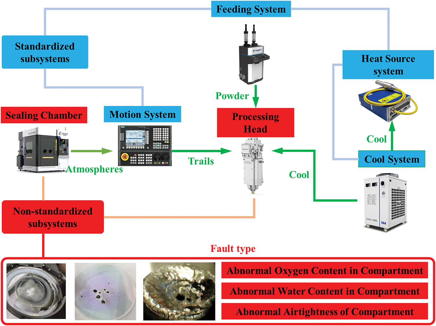
Figure 1: Additive manufacturing equipment frame diagram

Based on historical fault information and manual experience, the fault characteristics of processing head and sealing chamber failures were classified into five categories:

(1)   Abnormal processing head nozzle temperature: When the nozzle temperature exceeds the normal operating range, it may lead to nozzle burnout or other malfunctions.

(2)   Abnormal processing head protective glass temperature: When the protective glass temperature exceeds the normal operating range, it may cause damage to the protective glass or other malfunctions.

(3)   Abnormal oxygen contents in the sealing chamber: When the oxygen content in the sealing chamber exceeds the normal range, it may result in reduced laser efficiency or affected laser processing quality.

(4)   Abnormal humidity in the sealing chamber: When the water content in the sealing chamber exceeds the normal range, it may lead to equipment corrosion or reduced laser efficiency.

(5)   Abnormal airtightness of the chamber: When there is an abnormal pressure difference between the sealing chamber and the external environment, it may result in gas leaks and affect the laser processing process.

2.2 Fault Classification Theory

The PCSV asymptotic classification principle integrates Principal Component Analysis (PCA) and Support Vector Machine (SVM) for feature reduction and classification. PCA utilizes statistical measures to reduce data dimensionality while preserving essential variance, whereas SVM optimally classifies the data by maximizing the margin between different classes. In metal additive manufacturing process monitoring, sensor data often have missing values due to environmental disturbances or acquisition interruptions. This study uses the K Nearest Neighbor-based multivariate interpolation method (KNNImputer) to deal with the missing values as shown in Eq. (1):

x^i=∑j=1kwjxj∑j=1kwj,wj=1d(xi,xj)+ε(1)

where k denotes the number of nearest neighbors and d(⋅) is the Euclidean distance metric, which preserves the coupling between process parameters through feature space similarity. Compared with the traditional mean interpolation, this method can better preserve the original data distribution characteristics and provide a complete input matrix for the subsequent PCSV.

Eq. (2) assumes that the signal follows an F-distribution with degrees of freedom (n1, n2):

f(x)={Γ(n1+n22)Γ(n12)Γ(n22)(n1n2)(n1n2x)n12−1(1+n1n2x)n1+n22,x≥00,x<0(2)

PCA essentially takes the direction with the highest variance as the main feature. A variance is used to define the spacing of the samples. The larger variance means a larger sparser distribution and a smaller denser distribution. The Eq. (3) for variance is as follows:

Var(x)=1m∑i=1m(xi−x¯)2(3)

where m is the number of data points, xi is each data point, and x¯ is the mean. By selecting the direction of maximum variance, PCA ensures that the retained principal components effectively capture the most significant structural variations in the data. This is particularly useful in fault diagnosis in metal additive manufacturing, where defect-related variations may be embedded in complex, high-dimensional datasets. However, while PCA efficiently reduces dimensionality and removes noise, In the field of fault diagnosis in metal additive manufacturing, where fault samples are small, SVM is considered an effective method. It achieves data classification by finding a hyperplane that maximizes the margin between excellent performance for high-dimensional data and nonlinear relationships.

SVM is effective in fault classification, especially when fault samples are sparse. It seeks an optimal hyperplane that maximizes the margin between different classes. An arbitrary hyperplane can be defined as Eq. (4).

wTx+b=0(4)

where w is the weight vector, x is the input feature vector, and b is the bias term.

The formula for the distance from a point (x,y) in two dimensions to the line Ax+By+C is Eq. (5).

d2=|Ax+By+C|A2+B2(5)

After expansion into n-dimensional space, the distance from the point x=(x1,x2,…xn) to wTx + b = 0 is Eq. (6).

dn=|wTx+b|‖w‖(6)

of which:

‖w‖=w12+…wn2(7)

According to the definition of a support vector, the distance from the support vector to the hyperplane is d, and the distance from other points to the hyperplane is greater than d. So, Eq. (8) is subject to the constraint.

{wTx+b≥1,y=1wTx+b≤−1,y=−1(8)

To maximize the margin, the optimization problem is formulated as Eq. (9).

{y(wTx+b)≥1min12‖w‖2s.t(9)

where y represents the class labels. The advantage of SVM in metal additive manufacturing fault diagnosis is its capability to handle high-dimensional and nonlinear relationships through kernel functions. However, SVM’s performance is highly dependent on appropriate kernel selection and may require extensive computational resources for large datasets. Represents the class labels. The advantage of SVM in metal additive manufacturing fault diagnosis is its capability to handle high-dimensional and nonlinear relationships through kernel functions. However, SVM’s performance is highly dependent on appropriate kernel selection and may require extensive computational resources for large datasets.

3  Additive Manufacturing Fault Diagnosis Procedure Based on PCSV

3.1 Overview

As shown in Fig. 2, the PCSV asymptotic classification fault diagnosis method is divided into two stages.

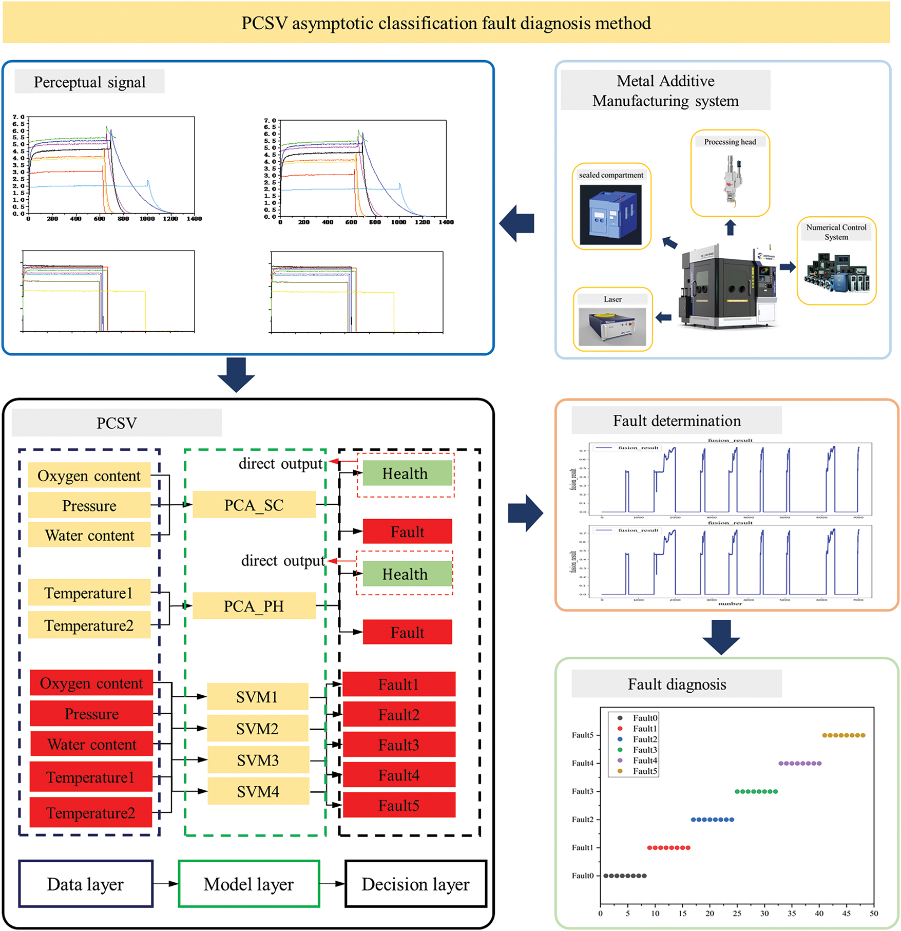
Figure 2: Overview of the fault diagnosis based on PCSV asymptotic classification

The first stage is data acquisition and fault determination. Data acquisition is to provide a database for fault diagnosis. The PCA models are used for preliminary screening of sensor data, excluding clearly normal data.

A simulated sealing chamber and an actual processing head are constructed, and oxygen analyzers, water analyzers, temperature sensors, airflow sensors, and pressure sensors are installed on the equipment. The role of these sensors is to collect key parameters related to the AM process, providing rich analog and digital data for subsequent fault diagnosis. Feature extraction is performed for five types of sensors. Through the analysis of feature data, two principal component analysis (PCA) models for the sealing chamber and processing head are constructed. The PCA models process the data dimensional reduction, which extracts the most representative features and lays the foundation for fault diagnosis.

Then, the left data labeled as abnormal is input into a support vector machine (SVM) model for further fault determination. The SVM model can effectively identify complex and nonlinear features, thereby improving the accuracy of fault diagnosis. Through the PCSV asymptotic fault classification method, timely diagnosis of faults can be achieved while ensuring the normal operation of the equipment.

3.2 Procedure

AM equipment is a highly integrated manufacturing system with multiple functional modules, and the process data is characterized by multiple sources and multiple data types. As industrial manufacturing equipment, it also faces the problem of high data redundancy. Therefore, to improve the accuracy and efficiency of additive manufacturing fault diagnosis. a PCSV asymptotic classification fault diagnosis method is proposed.

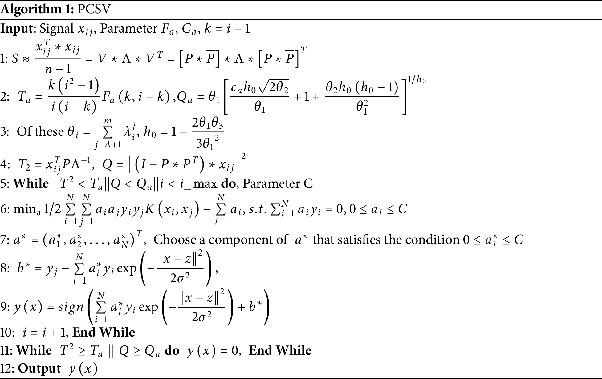
As shown in Algorithm 1, first, PCSV uses a recursive scheme for the initial decomposition of multiple signals, so the signals cannot be continuously updated. The purpose of using the recursive scheme is only to achieve the initial decomposition of the signal. Then, T2 and Q statistics are used for fault determination by calculating the threshold limits of the stencil data. Finally, PCSV introduces the Gaussian kernel function, which reduces the computational difficulty by mapping the low-dimensional parameters to the higher ones and turning the nonlinear parameters into linearly differentiable ones. The penalty function C is set to avoid model overfitting.

4  Result and Discussion

4.1 Experimental Setup

To verify the validity of the PCSV model, this study builds an additive manufacturing fault diagnosis hardware system. It aims to collect data under multiple fault conditions. The structure of the experimental setup is shown in Fig. 3. The system simulates different scenarios of sealed chamber leakage and processing head failure by accurately controlling a variety of physical variables, thus verifying the performance of the PCSV model in practical applications. The experimental setup includes the following key components:

(1)   Sealing chamber: Used to simulate the sealing problem in the additive manufacturing process, the ball valve controls its opening and closing to simulate the leakage phenomenon of the sealing chamber.

(2)   Processing head: The processing head fault is simulated by adjusting the cooling water flow, reflecting the abnormalities of the cooling system and its impact on the machining process.

(3)   Sensor network: water content, oxygen content, and pressure sensors are installed inside the sealing chamber to monitor the sealing status and gas leakage in real time; temperature sensors and cooling water flow sensors are installed on the machining head and its protective mirror to obtain the temperature change and cooling effect of the processing head.

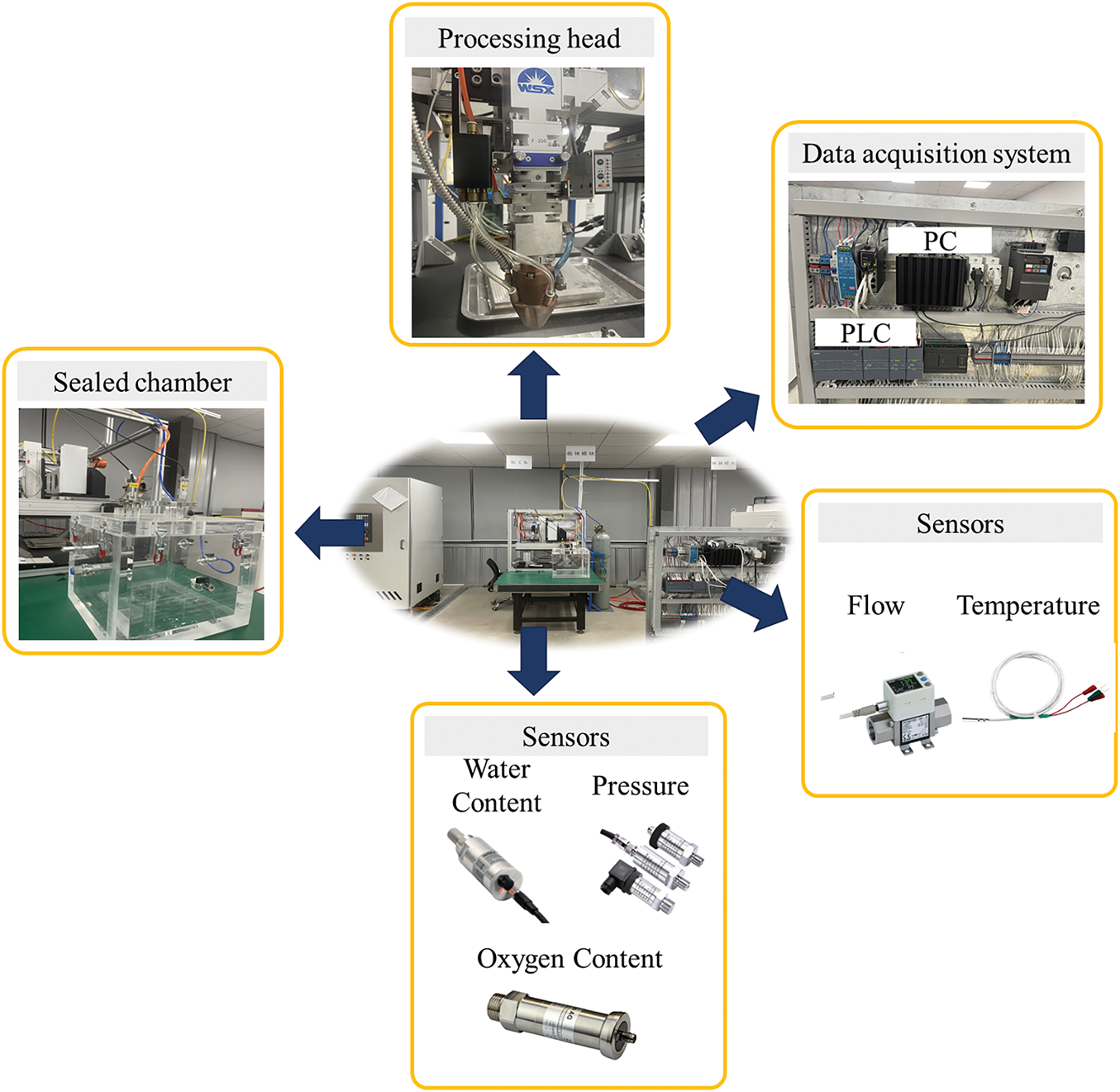
Figure 3: Experimental verification diagram

The specific experimental procedure is as follows:

(1)   Firstly, the system will periodically collect the characteristic parameters of the sealing chamber and the processing head with a sampling frequency of 500 ms. These data include water content, oxygen content, temperature, flow rate, pressure, etc., which will be the input features for the subsequent fault diagnosis model.

(2)   In order to simulate the leakage problem of the sealing chamber, the leakage level of the sealing chamber is adjusted by rotating the ball valve during the gas washing process. As the rotation angle increases, the leakage level gradually increases, and the sensors capture changes in water and oxygen content and pressure to provide a basis for subsequent fault identification. Experiments for each leakage level were conducted over multiple periods to collect multidimensional data and analyze the effect of leakage on different parameters.

(3)   On the processing head module, experiments were conducted to simulate processing head failure through three different sets of cooling water flow settings. Each set of experiments increases the degree of cooling system failure by gradually adjusting the water-cooling flow valve and collecting data on the temperature variation of the processing head. Different cooling water flow rates will affect the temperature distribution of the processing head, further affecting the accuracy and quality of additive manufacturing. By adjusting the size of the flow rate, different states ranging from minor to severe faults can be simulated, thus testing the diagnostic capability of the model at different levels of fault.

Through experiments, this study constructed a complete dataset. It covers the normal operating conditions of the seal chamber and the processing head as well as their fault conditions. The dataset contains different types of data collected by a variety of sensors, including parameters such as water content, oxygen content, pressure, temperature variation, and cooling water flow. By analyzing these parameters, different fault modes can be effectively identified and distinguished. Fig. 4 shows a typical data template of the sealing chamber and processing head under normal operating conditions, reflecting the stability and regularity of each parameter. Under normal operating conditions, the data show a relatively smooth trend with no obvious abnormal fluctuations. Fig. 5 presents a time-domain plot of all the data collected in the experiment, demonstrating the trend of the data from each sensor under different fault states. By comparing the data of normal and abnormal states, it can be clearly seen that the parameters monitored by the sensors undergo significant fluctuations when a fault occurs, especially some prominent peak changes.

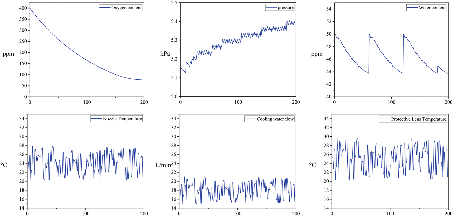
Figure 4: Normal operation data template

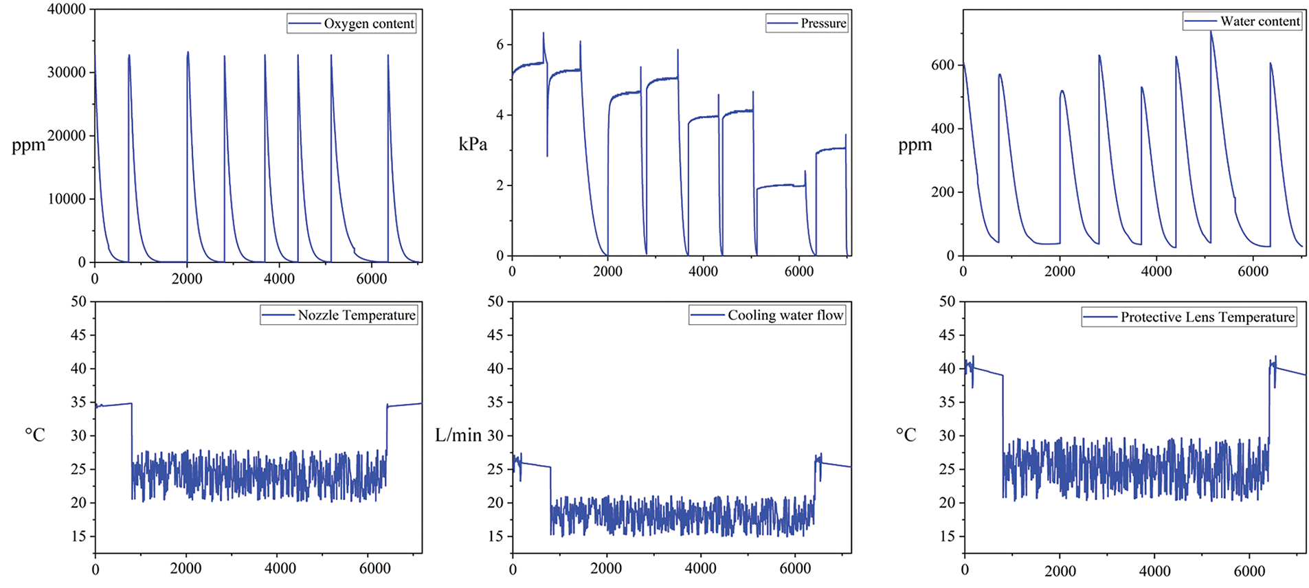
Figure 5: Time-domain plot of experimental data

For example, the readings of the water content, oxygen content, and pressure sensors change rapidly when there is a leakage failure in the seal chamber, while the values of the temperature and cooling water flow sensors show significant abnormalities when there is a fault in the processing head. These abrupt changes in characteristics provide a strong basis for subsequent fault diagnosis.

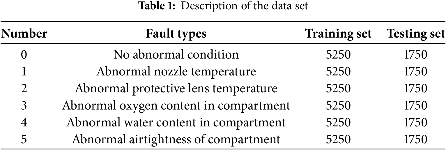
As shown in Table 1, seal chamber and processing head faults were categorized into six categories, each of which was coded based on 0 through 5. These categories include a variety of common fault types such as seal chamber leakage faults and abnormal cooling water flow in the processing head. By labeling and categorizing different faults, the experiment provides detailed labeling data for the training and validation of the PCSV model, which helps the model to accurately identify various types of faults. In order to validate the accuracy and efficiency of the PCSV model in fault diagnosis, all the collected data were divided into a training set and a test set in the ratio of 7:3. 70% of the data were used for the training of the model so that it could learn enough features and laws, while the remaining 30% of the data were used as a test set for evaluating the performance of the model in actual fault diagnosis.

4.2 Fault Diagnosis

Tuning is a key part of model optimization, and Table 2 presents the results of the PCSV model after tuning. In this model, the two principal components were selected based on their correspondence to the two functional modules of additive manufacturing, the processing head and the seal chamber. These components were chosen as they together explain 100% of the variance in the data, ensuring that dimensionality reduction reduces computational complexity while preserving critical information. This approach enables the model to process high-dimensional data more efficiently while minimizing information loss from excessive dimensionality reduction. The Gaussian (RBF) kernel function was selected for nonlinear mapping due to its ability to effectively handle complex and nonlinearly separable data distributions. This choice was made after evaluating multiple kernel functions, with the Gaussian kernel demonstrating superior performance in capturing intricate data patterns. The regularization parameter C was set to 1.0, as determined through empirical testing and cross-validation. A lower C value helps control overfitting by allowing more flexibility in separating data points while ensuring a balance between the model’s error on the training set and its generalization ability on the test set. The initial number of samples was set to 10, and the number of optimization iterations was limited to 30, based on an analysis of convergence behavior. These values were chosen to ensure an efficient search for optimal hyperparameters within a reasonable computational time. The batch size of 32 was selected to provide a balance between model stability and computational efficiency, allowing the model to utilize diverse data samples in each update while maintaining manageable memory usage. The batch size of 32, the learning rate of 0.01, and iteration limits were determined through progressive scaling experiments. A learning rate ablation study demonstrated this setting achieved 98% of maximum convergence speed while maintaining loss stability (σ2 < 0.02), with larger rates (>0.05) causing oscillatory behavior in gradient descent.

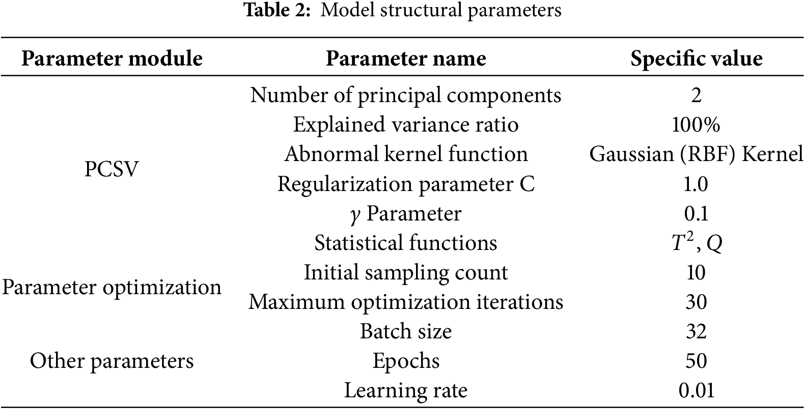
Fig. 6 depicts the process of Algorithm 1 (1–5). Due to the sealing chamber and processing head being two distinct modules of additive manufacturing equipment and their characteristics being unrelated, it is necessary to establish separate PCA models to determine if they have faults. The PCA model for the processing head is named CASE_PH, and the PCA model for the sealing chamber is named CASE_SC. After training, the T2 and Q statistic limits for normal data are calculated. As shown in Fig. 6a,b, T2 and Q limits are 300.89 and 3.8, respectively. For CASE_PH, T2 and Q limits for CASE_PH are 6.3 and 0.0014, respectively.

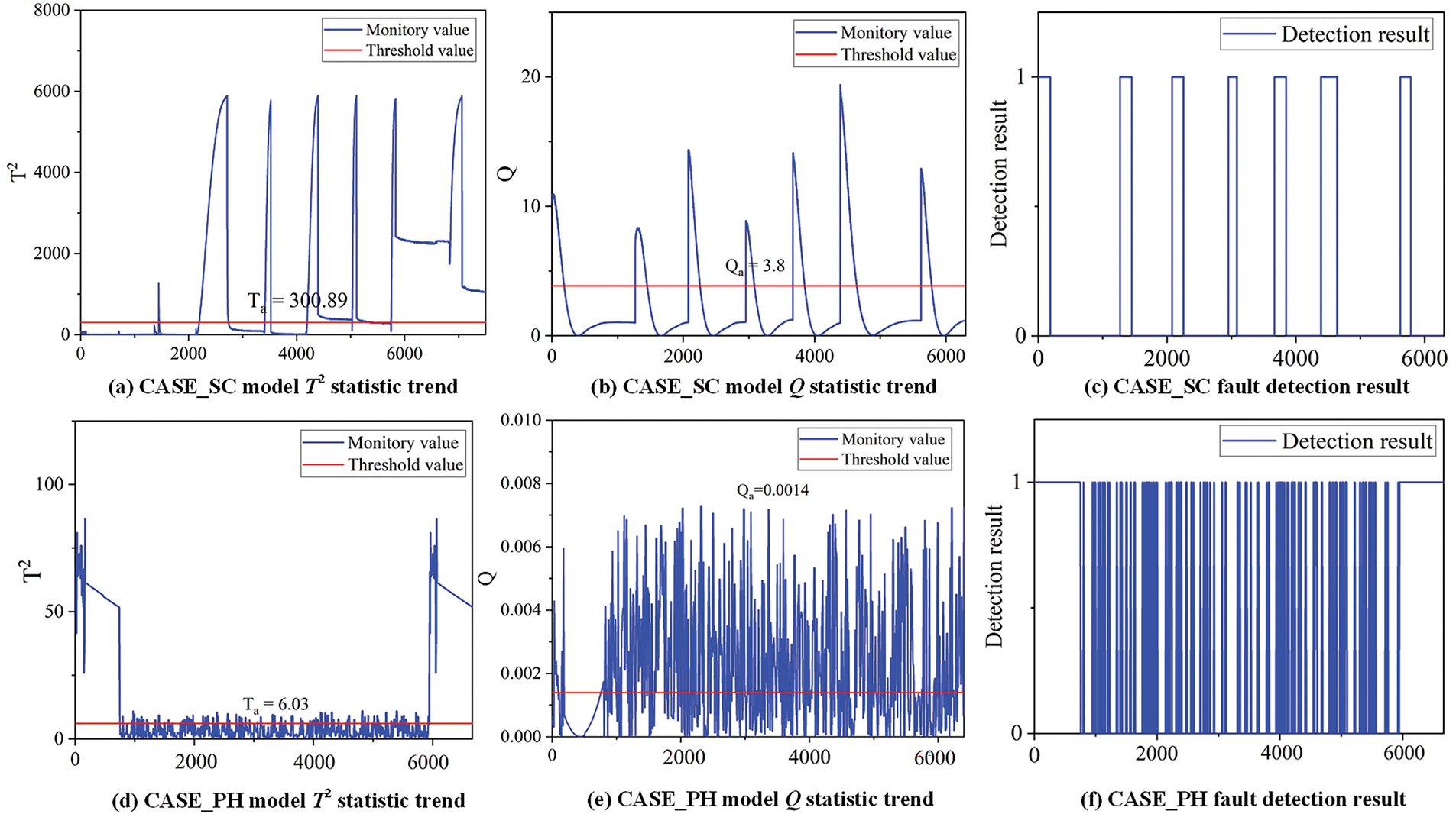
Figure 6: Fault determination visualization

Next, a test set is introduced to verify the PCA model. The test set includes data from both the sealing chamber and processing head under normal and fault conditions. During the testing, the PCA model learns the characteristics of the equipment under normal conditions from the data in the training set, enabling it to identify abnormal data in the test set. After training is complete, the trained PCA model is used to analyze the data in the test set. For each data point in the test set, its scores T2 and Q statistics under the PCA model are calculated and compared to the predefined thresholds. The accuracy of fault determination is 100%. The fault detection results are illustrated in Fig. 6c,f.

Finally, the data are labeled as normal and abnormal after PCA fault detection. In Fig. 6c,f, a fault determination result of 1 means that the system is abnormal. On the contrary, a fault determination result of 0 means that the system is normal. As shown in Fig. 7, The faulty data is then input into the SVM model for multi-classification.

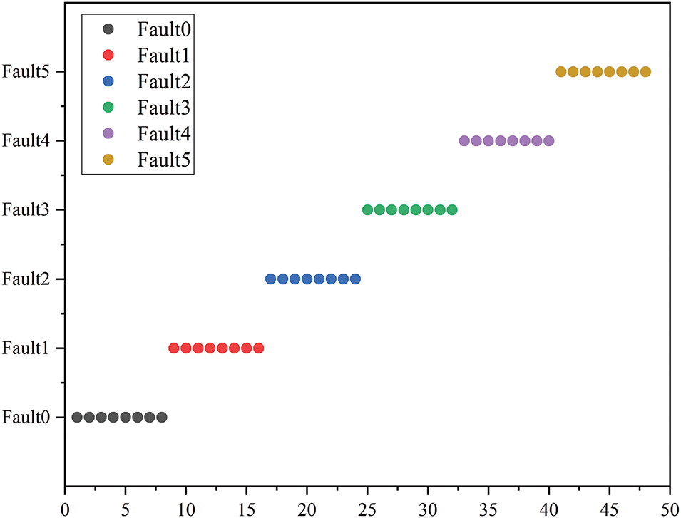
Figure 7: PCSV model classification results visualization

4.3 Comparative Analysis

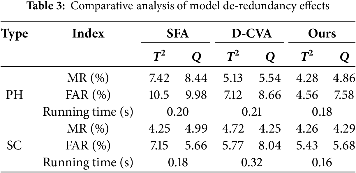
As shown in Eqs. (10) and (11), to further verify the fault diagnosis ability of PCSV, this study compares and analyzes with other methods from the two levels of redundancy and fault diagnosis. In terms of redundancy, SFA and D-CVA were selected for comparison with PCSV. The redundancy performance of the model is judged from three indicators: miss rate (MR), false alarm rate (FAR), and running time.

NDR=NFPNTN+NFP×100%(10)

FAR=NFNNTP+NFN×100%(11)

In order to eliminate the interference of random factors, the above comparison experiment was repeated 10 times, and the average of the 10 experiments was used to evaluate the performance of the model. The training set and test set are also configured according to 3:1. As shown in Table 3, compared with SFA and D-CVA, PCSV’s T2 and Q statistic parameters MR are reduced by 1.57, 2.14, and (0.66, 0.32) on average, indicating that PCSV has fidelity for the source data. Compared with SFA and D-CVA, The T2 and Q statistical parameters of PCSV are reduced by 3.83, 1.19, and 1.45, 1.72 on average, indicating that PCSV had higher accuracy. Compared with SFA and D-CVA, PCSV running time is lower, indicating that the model has better timeliness.

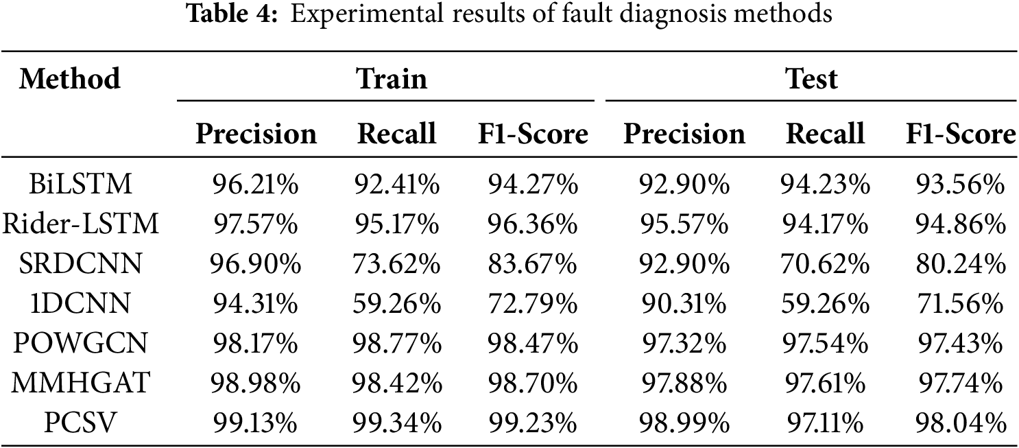
To verify the comprehensive performance of PCSV, Bidirectional long short-term memory neural network (BiLSTM) and Rider-LSTM [27] of recurrent neural networks, Stackable Residual Deep Convolutional Neural Network (SRDCNN), Lightweight one-dimensional convolutional neural network (1DCNN) of convolutional neural networks [28], Pruned-Optimized Weighted Graph Convolutional Network (POWGCN) [29] of state-of-the-art, Multi-Sensor Multi-Head Graph Attention Network (MMHGAT) [30] are selected as the comparison objects in this study. The training set and test set are also configured according to 3:1. The specific model building is as follows: (1) BiLSTM is designed to capture temporal dependencies in both forward and backward directions. The network comprises 2 bidirectional LSTM layers with hidden state dimension H, enabling sequential feature extraction while maintaining contextual awareness. (2) Rider-LSTM is a hybrid deep learning architecture integrating LSTM with attention mechanisms and convolutional operations. The model includes 2 convolutional layers for local pattern extraction, 2 max-pooling layers for downsampling, and 2 attention modules to focus on critical temporal segments. (3) SRDCNN leverages residual connections to enhance gradient flow in deep layers. The network stacks 2 residual blocks, each containing 2 convolutional layers with kernel size K and channel dimension C, followed by 2 pooling layers for hierarchical feature abstraction. (4) 1DCNN optimized for sequence processing. The architecture consists of 2 convolutional layers with kernel size K and channel dimension C, coupled with 2 global max-pooling layers to reduce spatial redundancy and retain salient features. (5) POWGCN to model relational dependencies in non-Euclidean data. The network utilizes 2 graph convolution layers with feature dimension D, dynamically aggregating neighborhood information through edge connections (E), and adopts spectral filtering for robust graph representation. (6) MMHGAT integrates multi-head attention mechanisms for heterogeneous graph learning. The model incorporates 2 multi-head graph attention layers with H attention heads, node embedding dimension D, and adaptive edge weighting to capture complex node interactions in multi-modal graphs.

As shown in Fig. 8 and Table 4. The highest training accuracy is PCSV (99.13%), followed by MMHGAT (98.98%) and POWGCN (98.17%), which indicate that these models fit well on the training set. In terms of test accuracy, PCSV is the highest (99.34%), followed by POWGCN (98.77%) and MMHGAT (98.42%), which indicates that these models are more capable of generalization, whereas 1DCNN (59.26%) and SRDCNN (73.62%) perform significantly lower than the training set on the test set, and may be overfitting. The combined comparison of Precision, Recall, and F1-score shows that PCSV performs the best on Precision (98.99%) and F1-score (98.04%), which indicates that the model maintains a high level of accuracy and stability in the classification task. The Precision of POWGCN and MMHGAT, Recall, and F1-score are also higher, indicating that the graph neural network class of methods performs superiorly in this task. The Recall of SRDCNN and 1DCNN is significantly lower than that of the other models, indicating that they perform weakly in capturing the correct category. The Precision, Recall, and F1-scores are all close to 98%, indicating that these models perform consistently in the categorization task. The Recall of SRDCNN and 1DCNN is significantly lower, indicating that these two models perform poorly in terms of recall, which may lead to the problem of missed detection.

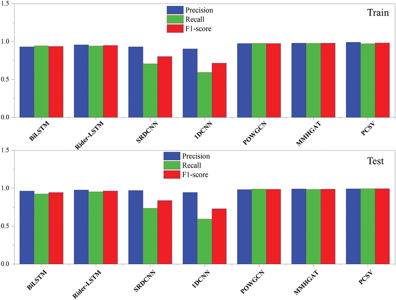
Figure 8: Comparison chart of methods

As shown in Table 5, In the comparative analysis of computational complexity and model efficiency, the performance characteristics of the models show significant differences. The time complexity of both SRDCNN and 1DCNN models based on convolutional neural networks constitutes an O (TKC2) relationship with the sequence length (T), convolutional kernel size (K), and the number of channels (C). Notably, although both have the same time complexity, 1DCNN achieves faster operation speed (0.68 s vs. 0.72 s) by reducing the parameter count accumulation due to the deep residual structure by a better space complexity design (O (KC2) vs. O (KC2L) for SRDCNN).

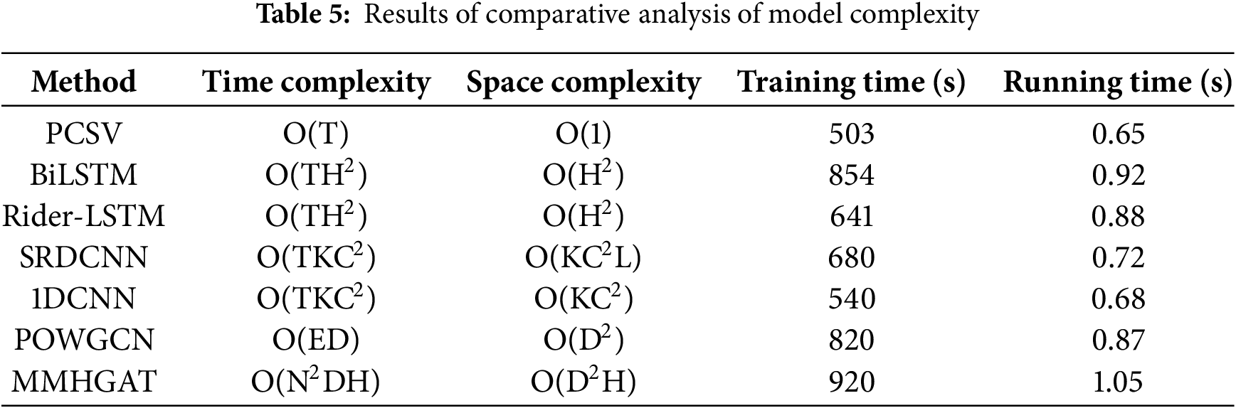
For graph neural networks, the time complexity of POWGCN is mainly constrained by the number of edges (E) and feature dimension (D) (O (ED)), while the multi-head attention mechanism of MMHGAT creates a complexity bottleneck of O (N2DH), which stems from the fact that it needs to compute the H-head attention for N nodes. The experimental data show that the training elapsed time (920 s) and inference time (1.05 s) of MMHGAT are significantly higher than that of POWGCN (820 s/0.87 s), which fully verifies the validity of the theoretical complexity analysis. In the field of sequence modeling, the computational efficiency of BiLSTM and Rider-LSTM significantly lags behind that of the PCSV model with O (T) time complexity due to the O (TH2) complexity brought by the hidden layer dimension H. The computational efficiency of BiLSTM and Rider-LSTM is significantly higher than that of the PCSV model with O (T) time complexity. This difference is especially significant in the training phase, where PCSV achieves a double optimization of training time (503 s) and inference time (0.65 s) under its concise architectural design.

A comprehensive evaluation of accuracy and efficiency shows that while MMHGAT and POWGCN can achieve high accuracy comparable to PCSV (>98.5%), their complex graph computation structure leads to an increase in training cost by 32%–41%. In particular, the MMHGAT model faces real-time challenges in equipment troubleshooting scenarios due to the need to maintain D2H-scale attention parameters. In contrast, PCSV fully validates its engineering applicability in additive manufacturing fault diagnosis scenarios by innovatively fusing temporal feature extraction and parameter space compression techniques, which ensures 98.99% diagnostic accuracy while controlling the inference latency at the millisecond level.

5  Conclusion

A multi-sensor and PCSV asymptotic classification fault diagnosis method is proposed for fault detection in additive manufacturing, particularly in scenarios such as turbine blade laser cladding, precision mold repair, and aluminum alloy structural component printing. The method integrates Principal Component Analysis (PCA) for fault detection and Support Vector Machines (SVM) for fault classification, ensuring accurate and efficient diagnosis. Experimental results confirm its effectiveness, making it a valuable tool for industrial applications.

The PCSV asymptotic classification method introduces two key innovations: (1) Adaptive Feature Selection Mechanism: Dynamically identifies and prioritizes relevant features at each diagnostic stage, reducing data redundancy and improving efficiency. For example, in turbine blade laser cladding, where temperature fluctuations and powder distribution inconsistencies can lead to bonding defects, this mechanism enhances fault detection accuracy by adjusting feature selection based on real-time process variations. (2) Hierarchical Decision-Making Framework: Enables progressive fault classification, starting with binary classification (normal vs. abnormal) and refining into multi-class fault diagnosis. This is particularly beneficial in precision mold repair via directed energy deposition (DED), where defects such as excessive material buildup, insufficient fusion, or layer misalignment can be progressively identified and classified, improving repair quality. Additionally, in aluminum alloy structural component printing, this framework enhances computational efficiency by distinguishing surface roughness anomalies, internal porosity, and residual stress-induced deformations, ensuring real-time process optimization. By addressing specific fault diagnosis challenges in these additive manufacturing applications, such as material deposition inconsistencies, laser energy fluctuations, and stress-induced cracking, this method enhances its practicality and applicability for high-precision manufacturing environments.

The proposed method still has room for improvement. (1) The current approach is trained based on fixed parameters and fault data from specific equipment, but real-world operating conditions may vary, causing changes in equipment performance. To enhance the robustness of fault diagnosis across different operating conditions, future work could focus on integrating adaptive mechanisms into the model. One possible direction is to incorporate online learning techniques, such as incremental learning or transfer learning, to continuously update the model based on real-time environmental data. Additionally, sensor fusion methods could be employed to dynamically adjust fault diagnosis thresholds in response to variations in temperature, humidity, or load. These techniques could be combined with the existing PCSV model by introducing an adaptive weighting mechanism that assigns different importance to feature components based on environmental conditions. Furthermore, Bayesian optimization or reinforcement learning could be explored to fine-tune model parameters dynamically, ensuring optimal performance across diverse operating scenarios. (2) The current method addresses fault detection for individual devices, but in practical applications, multiple devices often need to be monitored simultaneously. Future research could explore the development of an integrated fault diagnosis system that enables real-time monitoring and predictive maintenance across a network of devices. A potential framework for this system could involve a hierarchical architecture, where edge computing devices collect and preprocess local sensor data before transmitting key features to a centralized cloud or edge server via an industrial communication protocol such as MQTT or OPC UA. A unified fault diagnosis strategy could be implemented using a combination of federated learning and ensemble models, allowing each device to contribute to a shared model while retaining device-specific adaptations. Additionally, to account for interactions between devices, graph neural networks (GNNs) or dynamic Bayesian networks (DBNs) could be used to model dependencies and correlations between devices, enabling more accurate fault predictions. This integrated approach would enhance system-wide reliability by providing early warnings of faults that could propagate across interconnected devices.

Acknowledgement: Thanks to all team members for their work and contributions.

Funding Statement: This work is supported in part by the National Key R&D Program of China Grant 2022YFB4602200.

Author Contributions: The authors confirm their contribution to the paper as follows: study conception and design: Fei Xing, Qiang Wang, Jianjun Shi, Lingfeng Wang; data collection: Lingfeng Wang; algorithm design: Lingfeng Wang; analysis and interpretation of results: Lingfeng Wang, Jianjun Shi; experimental environment: Dongbiao Li; draft manuscript preparation: Lingfeng Wang. All authors reviewed the results and approved the final version of the manuscript.

Availability of Data and Materials: The data used to support the findings of the study are available from the corresponding author upon request.

Ethics Approval: Not applicable.

Conflicts of Interest: The authors declare no conflicts of interest to report regarding the present study.

References

1. García-Marín E, Masa-Campos JL, Sánchez-Olivares P, Ruiz-Cruz JA. Evaluation of additive manufacturing techniques applied to ku-band multilayer corporate waveguide antennas. IEEE Antennas Wirel Propag Lett. 2018;17(11):2114–18. doi:10.1109/LAWP.2018.2866631. [Google Scholar] [CrossRef]

2. Wen X, Yu Y, Shi G, Wang Z, Cheng Q, Li Y, et al. WR-3.4 band waveguide and bandpass filters using copper additive manufacturing. IEEE Trans Microw Theory Tech. 2023;71(3):1190–20. doi:10.1109/TMTT.2022.3217772. [Google Scholar] [CrossRef]

3. Verploegh S, Coffey M, Grossman E, Popović Z. Properties of 50-110-GHz waveguide components fabricated by metal additive manufacturing. IEEE Trans Microw Theory Tech. 2017;65(12):5144–53. doi:10.1109/TMTT.2017.2771446. [Google Scholar] [CrossRef]

4. Percaz JM, Hussain J, Arregui I, Teberio F, Benito D, Martin-Iglesias P, et al. Synthesis of rectangular waveguide filters with smooth profile oriented to direct metal additive manufacturing. IEEE Trans Microw Theory Tech. 2023;71(7):3081–101. doi:10.1109/TMTT.2023.3245683. [Google Scholar] [CrossRef]

5. Gumbleton R, Cuenca JA, Hefford S, Nai K, Porch A. Measurement technique for microwave surface resistance of additive manufactured metals. IEEE Trans Microw Theory Tech. 2021;69(1):189–97. doi:10.1109/TMTT.2020.3035082. [Google Scholar] [CrossRef]

6. Yang H, Wen X, Yu Y, Shi G, Wang Z, Li Y, et al. A D-Band waveguide diplexer based on copper additive manufacturing. IEEE Trans Compon Packag Manuf Technol. 2023;13(8):1271–77. doi:10.1109/TCPMT.2023.3298966. [Google Scholar] [CrossRef]

7. Zhang P, Li K, Yu S, Yu D. A novel fault diagnosis technique of interturn short-circuit fault for SRM in current chopper mode. IEEE Trans Ind Electron. 2022;69(3):3037–46. doi:10.1109/TIE.2021.3066917. [Google Scholar] [CrossRef]

8. Huo M, Luo H, Cheng C. Subspace-aided sensor fault diagnosis and compensation for industrial systems. IEEE Trans Ind Electron. 2023;70(9):9474–82. doi:10.1109/TIE.2022.3215823. [Google Scholar] [CrossRef]

9. Shi X, Gu H, Yao B. Fuzzy bayesian network fault diagnosis method based on fault tree for coal mine drainage system. IEEE Sens J. 2024;24(6):7537–47. doi:10.1109/JSEN.2024.3354415. [Google Scholar] [CrossRef]

10. Zhang X, Li Y, Liu Y. Adaptive fault diagnosis and decision-making method based on multi-spectrum evaluation and fusion for traction motor bearings. IEEE Trans Instrum Meas. 2023;72:1–19. doi:10.1109/TIM.2023.3330226. [Google Scholar] [CrossRef]

11. Zhou Y, He Y, Xing Z. Vibration signal-based fusion residual attention model for power transformer fault diagnosis. IEEE Sens J. 2024;24(10):17231–42. doi:10.1109/JSEN.2024.3382811. [Google Scholar] [CrossRef]

12. Zhou Y, Dong Y, Tang G. Time-varying online transfer learning for intelligent bearing fault diagnosis with incomplete unlabeled target data. IEEE Trans Ind Inform. 2023;19(6):7733–41. doi:10.1109/TII.2022.3230669. [Google Scholar] [CrossRef]

13. Chen C, Wang T, Liu C. Lightweight convolutional transformers enhanced meta-learning for compound fault diagnosis of industrial robot. IEEE Trans Instrum Meas. 2023;72:1–12. doi:10.1109/TIM.2023.3277956. [Google Scholar] [CrossRef]

14. Binu D, Kariyappa BS. Rider-Deep-LSTM network for hybrid distance score-based fault prediction in analog circuits. IEEE Trans Ind Electron. 2021;68(10):10097–106. doi:10.1109/TIE.2020.3028796. [Google Scholar] [CrossRef]

15. Xue Q, Chen C, Fan W. PCA-Res2Net model-based method for damage detection of CFRP using electrical impedance tomography. IEEE Trans Instrum Meas. 2024;73(1):1–10. doi:10.1109/TIM.2023.3336759. [Google Scholar] [CrossRef]

16. Fan H, Lai X, Du S, Yu W, Lu C, Wu M. Distributed monitoring with integrated probability PCA and mRMR for drilling processes. IEEE Trans Instrum Meas. 2022;71(1):1–13. doi:10.1109/TIM.2022.3186081. [Google Scholar] [CrossRef]

17. Zhong K, Ma D, Han M. Distributed dynamic process monitoring based on dynamic slow feature analysis with minimal redundancy maximal relevance. Control Eng Pract. 2020;104(2):104627. doi:10.1016/j.conengprac.2020.104627. [Google Scholar] [CrossRef]

18. Ji H, Hou Q, Shao Y. Incipient fault detection for dynamic processes with canonical variate residual statistics analysis. Chemom Intell Lab Syst. 2024;252(12):105189. doi:10.1016/j.chemolab.2024.105189. [Google Scholar] [CrossRef]

19. Zhu H, Cheng J, Zhang C, Wu J, Shao X. Stacked pruning sparse denoising autoencoder based intelligent fault diagnosis of rolling bearings. Appl Soft Comput. 2020;88(99):106060. doi:10.1016/j.asoc.2019.106060. [Google Scholar] [CrossRef]

20. Niu G, Liu E, Wang X, Zhang B. A hybrid bearing prognostic method with fault diagnosis and model fusion. IEEE Trans Ind Inform. 2024;20(1):864–72. doi:10.1109/TII.2023.3265532. [Google Scholar] [CrossRef]

21. Chen J, Hu W, Cao D. A meta-learning method for electric machine bearing fault diagnosis under varying working conditions with limited data. IEEE Trans Ind Inform. 2023;19(3):2552–64. doi:10.1109/TII.2022.3165027. [Google Scholar] [CrossRef]

22. Rauber TW, de Assis Boldt F, Varejao FM. Heterogeneous feature models and feature selection applied to bearing fault diagnosis. IEEE Trans Ind Electron. 2015;62(1):637–46. doi:10.1109/TIE.2014.2327589. [Google Scholar] [CrossRef]

23. Guo L, Wang K, Wang T. Open-circuit fault diagnosis of three-phase permanent magnet machine utilizing normalized flux-producing current. IEEE Trans Ind Electron. 2024;71(4):3351–60. doi:10.1109/TIE.2023.3273254. [Google Scholar] [CrossRef]

24. Kong X, Yang Z, Luo J, Li H, Yang X. Extraction of reduced fault subspace based on KDICA and its application in fault diagnosis. IEEE Trans Instrum Meas. 2022;71:1–12. doi:10.1109/TIM.2022.3150589. [Google Scholar] [CrossRef]

25. Yang H, Wen X, Yu Y, Shi G, Wang Z, Li Y, et al. An open-circuit faults diagnosis method for MMC based on extreme gradient boosting. IEEE Trans Ind Electron. 2022;70(6):6239–49. doi:10.1109/TIE.2022.3194584. [Google Scholar] [CrossRef]

26. Chine W, Mellit A, Lughi V, Malek A, Sulligoi G, Pavan AM, et al. A novel fault diagnosis technique for photovoltaic systems based on artificial neural networks. Renew Energy. 2016;90(2188):501–12. doi:10.1016/j.renene.2016.01.036. [Google Scholar] [CrossRef]

27. Mohammad-Alikhani A, Nahid-Mobarakeh B, Hsieh MF. One-dimensional LSTM-regulated deep residual network for data-driven fault detection in electric machines. IEEE Trans Ind Electron. 2024;71(3):3083–92. doi:10.1109/TIE.2023.3265054. [Google Scholar] [CrossRef]

28. Sharma M, Maity T. Multisensor data-fusion-based gas hazard prediction using DSET and 1DCNN for underground longwall coal mine. IEEE Internet Things J. 2022;9(21):21064–72. doi:10.1109/JIOT.2022.3175724. [Google Scholar] [CrossRef]

29. Zhang X, Jiang L, Wang L, Zhang T, Zhang F. A pruned-optimized weighted graph convolutional network for axial flow pump fault diagnosis with hydrophone signals. Adv Eng Inform. 2024;60:102365. doi:10.1016/j.aei.2024.102365. [Google Scholar] [CrossRef]

30. Wang Z, Wu Z, Li TXM. Attention-aware temporal-spatial graph neural network with multi-sensor information fusion for fault diagnosis. Knowl-Based Syst. 2023;278(4):110891. doi:10.1016/j.knosys.2023.110891. [Google Scholar] [CrossRef]