
 Submit a Paper
 Propose a Special lssue
 Open Access
ARTICLE

Monitoring the Oil Tank Deformations for Different Operating Conditions
1 Interdisciplinary Research Center for Aviation and Space Exploration, King Fahd University of Petroleum and Minerals, Dhahran, 34463, Saudi Arabia
2 Department of Aerospace Engineering, King Fahd University of Petroleum and Minerals, Dhahran, 34463, Saudi Arabia
3 Department of Applied Geodesy, Kyiv National University of Construction and Architecture, Kyiv, 03037, Ukraine
* Corresponding Author: Roman Shults. Email:
(This article belongs to the Special Issue: Non-contact Sensing in Infrastructure Health Monitoring)
Structural Durability & Health Monitoring 2025, 19(6), 1433-1456. https://doi.org/10.32604/sdhm.2025.068099
Received 21 May 2025; Accepted 14 August 2025; Issue published 17 November 2025
 View Full Text
 Download PDF
Abstract
Oil tanks are essential components of the oil industry, facilitating the safe storage and transportation of crude oil. Safely managing oil tanks is a crucial aspect of environmental protection. Oil tanks are often used under extreme operational conditions, including dynamic loads, temperature variations, etc., which may result in unpredictable deformations that can cause severe damage or tank collapses. Therefore, it is essential to establish a monitoring system to prevent and predict potential deformations. Terrestrial laser scanning (TLS) has played a significant role in oil tank monitoring over the past decades. However, the full extent of TLS capabilities for oil tank monitoring has not yet been thoroughly investigated. This study aims to evaluate TLS’s abilities in detecting deformations of oil tanks under various operating conditions. The paper has two objectives: first, to examine the deformations of two vertical oil tanks over six years, and second, to investigate potential deformations of the tanks’ surfaces during filling. Each tank was scanned three times—in the years 2015, 2016, and 2021. Mathematical models and appropriate software were developed to determine the achievable accuracy of TLS monitoring. The anticipated monitoring accuracy was simulated based on the design parameters of the oil tanks. This accuracy was subsequently used to differentiate between deformations and measurement errors. The tank surface was approximated utilizing the cylinder equation for each monitoring epoch. Additionally, deformations were analyzed at different cross-sections with the appropriate circular approximations. The results indicated that both tanks exhibited no significant deformations within a range of less than 20 mm. For the empty tanks, the average radius decreased by 4 mm, without any changes in shape. The total spatial inclination of the oil tanks was calculated using cylinder equations at different monitoring epochs. In the final stage, the observed deformations were employed to simulate the strain-stress conditions of the oil tanks. Thus, this paper presents a complex technology and the results of oil tank monitoring by TLS under various operating conditions.Keywords
Monitoring engineering structures is crucial for their safe and efficient use throughout their entire life cycle. Industrial structures require utmost attention due to extreme functional conditions and the potential environmental impact in the event of a collapse. Oil tanks are integral to the oil industry, playing a significant role in the storage and transportation of crude oil. Therefore, precise and reliable monitoring of oil tanks is particularly important for safe operation. Under various loads, oil tanks may deform and change shape, leading to a loss of stability. The timely identification of expected deformations and the assignment of necessary structural interventions help prevent the risk of collapse. Oil tank monitoring can be organized using geospatial and geotechnical methods and technologies. To detect spatial displacements of oil tanks, including tank inclination, the primary approach relies on geospatial methods. These methods have evolved from traditional geodetic methods such as leveling [1–3] and geodetic resections [2–4] to contemporary monitoring technologies integrated with BIM [5]. Among these methods, total station surveying in reflectorless mode [6–9] is the most widely used. Despite its advantages, this method has significant drawbacks, notably slow surveying speed and low point density. Partially, these challenges were overcome by robotic total stations. However, the point density remains insufficient. The implementation of terrestrial laser scanning (TLS) has simplified the measurement process and increased data volume.
Today, TLS is widely used to monitor various engineering structures. However, little research has been conducted specifically on oil tank monitoring. It is worth mentioning studies that focus on similar research, particularly the monitoring of cooling towers [10,11] and historical buildings [12–14], which also have a similar geometry. TLS monitoring of tall structures such as chimneys [15] and wind towers [16] using TS can also be considered examples of cylindrical structure monitoring. However, the relationship between the height and width of these structures makes the simulation less stable compared to those with a more uniform ratio. Regardless of the structure type, scant attention has been given to measurement accuracy. Modern TLSs provide excellent accuracy, but only over short distances. Scanning large oil tanks from these short distances (up to 15 m) is not feasible. This brings us to a central question emerging from known studies: How can the accuracy of deformation determination be reliably estimated in advance? A reliable preliminary accuracy assessment will help in identifying tank deformations and distinguishing them from errors or measurement noise.
The primary challenge in tank monitoring lies in processing and analyzing TLS data. Generally, authors focus on deformation studies using tank cross-sections along the tank’s vertical axis [7,8]. These cross-sections are typically constructed at 1-m intervals [17–20]. Yet, this approach neglects potential local deformations, such as bulges. Previous studies have overlooked this issue. Furthermore, the overall deformation picture can be distorted due to loss of spatial detail. TLS data are presented as a highly dense point cloud, enabling us to simulate the entire tank surface and construct cross-sections at any desired location. However, processing TLS data is complex. The final outcome will depend on the chosen processing strategy and simulation algorithm. Some authors suggest using bicubic spline interpolation and other spline functions [9,21], non-uniform rational B-splines [22], or polynomial surfaces [23]. The ideal geometry of an oil tank is a circular cylinder. Thus, adequate approximation or interpolation should preserve the geometry as close to a circular cylinder as possible. Despite precise approximation, various spline or polynomial functions can generate an arbitrary surface that fits the point cloud according to specific optimization criteria. Yet, such approximations do not accurately represent the actual tank radius or inclination. The goal of monitoring is to determine both shape deformation and spatial displacement. For oil tanks, the primary spatial displacement is inclination. While previous studies [19,20] considered the algorithm for circular structure inclination, their idea was based solely on cross-section analysis. The most precise and reliable method for determining inclination is to analyze the orientation of the cylinder axis across observation epochs. Hence, the optimal approach is to approximate a point cloud with a cylinder surface and determine the parameters of this surface, including point coordinates on the cylinder axis, the direction vector of this axis, and the radius. Algorithms for cylinder approximation are outlined in [24–26]. Although many studies have addressed such approximation tasks, little attention has been paid to the implementation of these algorithms for monitoring problems. Therefore, the second aim of our research is to develop an algorithm and mathematical procedure for determining spatial displacements and deformations of oil tanks by approximating the TLS point cloud with a cylinder surface.
The final crucial step in the workflow is deformation analysis. This analysis should be conducted using structural mechanics methods. Studies such as [27,28] have investigated the role of the finite element method (FEM) for analyzing geospatial monitoring results. The authors in [12,13] have attempted to combine TLS results and FEM simulation. However, their analysis was conducted independently of monitoring results, relying solely on theoretical assumptions about the deformation process. Consequently, as a practical extension of these findings, we analyzed the deformations of oil tanks using FEM.
As a summary, we can highlight the following gaps in oil tank deformation monitoring that need to be addressed in future studies:
• Limited research exists on using TLS for oil tank monitoring, despite its widespread application in other structures.
• Current studies rely on vertical cross-sections at fixed intervals, which fail to detect local anomalies such as bulges.
• Few works have addressed the challenge of preliminary accuracy estimation to differentiate between actual deformations and measurement noise.
• Current surface approximation methods (splines, NURBS, polynomials) often fail to preserve the actual geometry of oil tanks (keep cylindricity), which limits their usefulness in spatial displacement analysis.
• The opportunities of cylinder approximation for detecting tank inclination and deformations remain underexplored.
• The integration of TLS results with structural mechanics methods, especially FEM, for detailed deformation analysis is rarely implemented in oil tank studies.
Based on this summary, in the presented paper, we
• Propose a TLS-based monitoring framework for oil tanks that addresses both shape deformation and spatial displacement (inclination).
• Provide a comprehensive monitoring flowchart that combines geospatial data processing and structural analysis techniques to improve oil tank safety and maintenance.
• Develop a preliminary accuracy estimation model to ensure reliable differentiation between actual deformations and noise.
• Implement an algorithm to determine tank inclination by analyzing the cylinder axis orientation between observation epochs.
• Integrate the traditional cross-section-based analysis with cylinder approximation and demonstrate the advantages of full-surface modeling.
• Apply FEM to evaluate the structural implications of detected deformations, enhancing the physical interpretation of geospatial data.
Overall, the aim of this study is to address the issue of oil tank geospatial monitoring using TLS data and advanced analysis methods. The paper is divided into five sections. Section 2 provides a brief overview of TLS data, monitoring technology, and data for further analysis. In Section 3, we present key methods used in our study. The section introduces a monitoring flowchart. The model of preliminary accuracy calculation is considered, and the mathematical model of an oil tank approximation is discussed. The algorithm for inclination determination is also included. Section 4 outlines the study results, detailing the findings of deformation and displacement analyses, as well as the FEM analysis with the results discussion. Section 5 deals with the conclusions.
The study utilized the results of TLS collected from scanning of two vertical cylindrical oil tanks, specifically Tanks No. 1 and No. 2 (Fig. 1). These tanks were scanned three times, and details about scanning time and tank status are provided in Table 1.
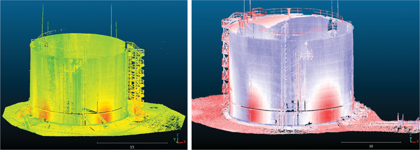
Figure 1: Point clouds of oil tanks No. 1 and No. 2
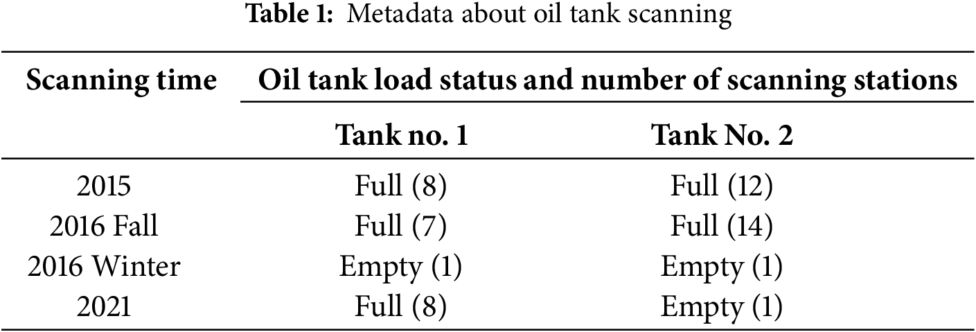
Thanks to these data, it became possible to determine the surface deformations of the tank surfaces over five years of operation and to investigate possible deformations of the tank surface during filling and draining processes. The average size of a point cloud at each observation epoch was approximately 20 million points. The number of scanning stations varied from seven to fourteen. For each tank, a local coordinate system was adopted, and no reference targets or networks were used. Scanning was performed using a FARO laser scanner, with an average scanning distance of 25 m to the object.
For further research, it is essential to understand the design parameters of the oil tanks. The studied tanks belong to the RVS-5000 class of vertical steel cylindrical tanks with a volume of 5000 m3. The design dimensions of RVS-5000 include an internal diameter of 20.920 m (radius 10.460 m) and a height of 14.900 m. Tanks of this class have ten vertical belts, with the lower belt having a thickness of 12 mm and the upper one 10 mm. The allowable deformations of the tank surface must not exceed ±1/1000 of the diameter, which is ±20.9 mm, and the allowable linear inclination value must be within ±1/200 of the tank height, i.e., the allowable inclination is ±74.5 mm.
The most challenging part of oil tank monitoring is the data analysis phase. This phase includes multiple analyses of deformations and other parameters. The analysis can be split into two stages: geometrical and finite element analysis. To make it clear, we summarized all monitoring stages into a general flowchart (Fig. 2).
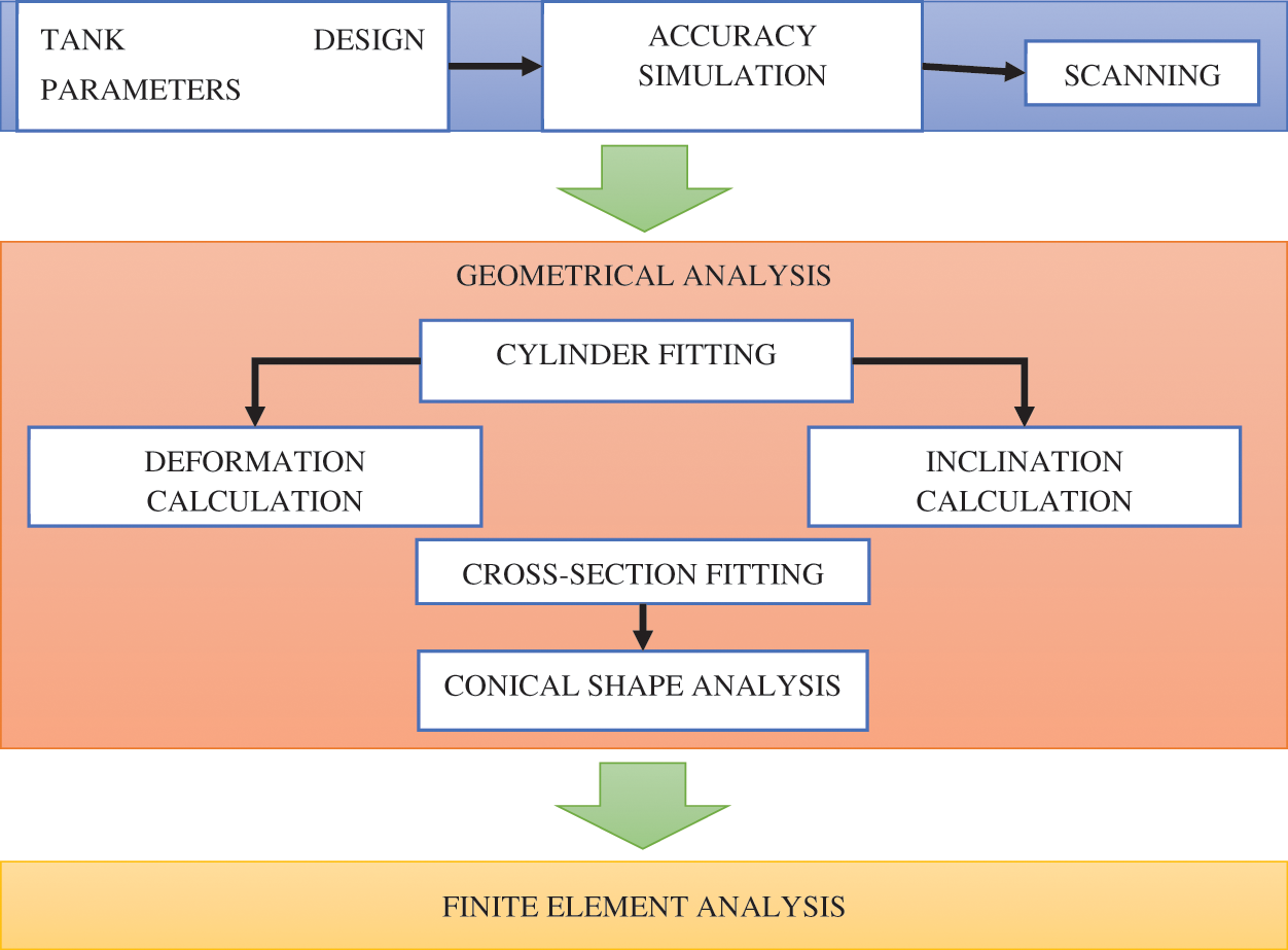
Figure 2: Monitoring flowchart
The monitoring begins with an analysis of the tank’s design parameters. This information helps determine the necessary values for the subsequent accuracy simulation. Typically, to simulate achievable TLS accuracy, we require the tank’s height, radius, wall thickness, allowable deformation, and expected environmental conditions during scanning, among other factors. After gathering this information, we proceed with a TLS accuracy simulation. The mathematical background of the accuracy calculation is explained in Section 3.2. The obtained accuracy multiplied by the square root of two provides the deformation determination accuracy. Based on this, we can select a laser scanner with suitable parameters (measurement range, accuracy, and laser beam properties, etc.). Once the accuracy and scanner are finalized, the scanning process can be carried out. In the flowchart, the scanning step also includes point cloud referencing and filtering. The resulting point cloud presents a nearly cylindrical surface that must be analyzed. To identify tank surface deformations, the point cloud is approximated using the equation of a cylinder surface. This is the initial stage for geometric analysis. The cylinder fitting procedure is described in Section 3.3. Fitting is performed using the least squares method, including calculation of the parameter covariance matrix. The deviations of the point cloud from the fitted cylinder across different observation epochs provide the deformation values. This analysis helps to identify changes in the tank surface. The overall displacement of the oil tank as a rigid body can be derived from the fitted cylinder parameters. Considering the very low likelihood of horizontal movement, the primary global displacement is expected to be the tank inclination. The algorithm for calculating inclination is provided in Section 3.4. To investigate the tank’s conicity, cross-sections are extracted from the point cloud and fitted with a 3D circle equation. Analyzing how the radius varies with height indicates potential tank conicity. Thus, the geometric analysis stage includes the determination of surface deformations, inclination, and conicity. The analysis of the cross-sections completes the overall geometric analysis. The second stage involves finite element analysis. For this, the tank’s design parameters and deformations from the geometric analysis are utilized.
To develop the model for preliminary accuracy calculation, we use the equations for single point coordinates determined by TLS (1):
The designators in (1) are clear from Fig. 3.
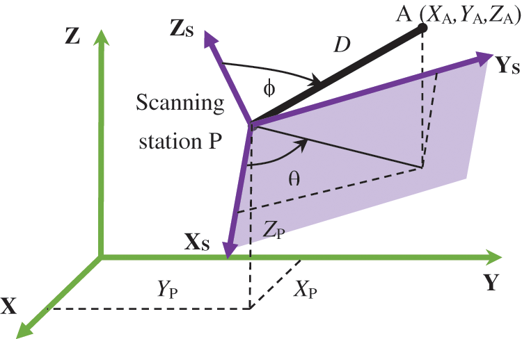
Figure 3: Geometry of TLS scanning from station P for point A
Let us apply the error propagation approach [29]. After differentiating Eq. (1) with respect to the parameters, we obtain the following matrix of partial derivatives:
To proceed with expressions for accuracy, we establish the matrix of RMSEs for measurements using the specification of the chosen laser scanner:
where:
Using the error propagation law, we obtain a covariance matrix
Typically, scanning must be conducted from multiple stations that need to be aligned with each other and/or with the established coordinate system. In this context, it is essential to consider the scanning station referencing errors resulting from the coordinate transformation, as well as any errors in the reference geodetic network. In laser scanning, the Helmert spatial coordinate transformation is applied under the condition that the scale factor is equal to one. Consequently, orientation errors are influenced by the errors of the scanning station rotation in space
Then, by utilizing the expressions for the Helmert coordinate transformation and deriving partial derivatives [30], we obtain an expression for calculating the laser scan referencing error
Finally, we obtain the following model for the preliminary calculation of the accuracy in determining displacements by the TLS, where the transition from errors in determining coordinates to errors in displacements
Expression (7)enables us to simulate the expected accuracy for any point on the scan. To implement the proposed method, we require a rough point cloud, which can be easily generated in this case based on the known geometry of the oil tank.
Since the ideal surface of a vertical oil tank is a cylinder, detecting deformations can be achieved by comparing the measured coordinates of points with the cylinder’s surface. This surface can be generated by fitting the cylinder to the point cloud. The explicit form of the cylinder equation is not suitable for approximation. Therefore, we employed a parametric axis-based model, which applies to a cylinder with an arbitrarily oriented axis (8).
where
Thus, the cylinder parametrization is presented by
where
The fitting procedure aims to optimize the following objective function (10) by using the least squares algorithm.
The effectiveness of the fitting is estimated using RMSE (11).
where
Covariance of the estimated parameters will be:
where
The expressions for the partial derivatives in (13) can be found in [30]. To derive the parameter accuracy, we use the diagonal elements of the covariance matrix (12).
This algorithm will be applied in the following sections to estimate cylinder parameters and to compute the expected deformations of an oil tank’s surface.
3.4 Cylinder Inclination between Observation Epochs
To determine the possible inclination of a tank between observations, we suggest applying a rigid transformation. Suppose that, after the fitting procedure, we have the vectors that determine the position and direction of the cylinder axis for two observation epochs. Therefore, we have two lines:
To compute the rotation R from normalized vectors
If
To find the rotation matrix, we use Rodrigues’ formula [14,31].
where
Then we can calculate the translation
The rotation matrix and respective angles about the axis in Euler form will be calculated as:
Special cases of rotation angles are discussed in [32]. The rotation angles determine the inclination of the oil tank in various directions between observation epochs.
4.1 Accuracy of Deformation Determination
To simulate accuracy, we use the main parameters of the scanner from its specifications to predict the expected accuracy for deformation determination using the equations from Section 3. A raw point cloud was generated based on the oil tank parameters (radius and height). The generated point cloud was treated as error-free. By selecting various positions of the scanning station, we obtained different distributions of point cloud accuracy. Previous studies suggest that the scanning distance is approximately 25 m. The results of the accuracy simulation for this distance are presented in Fig. 4.
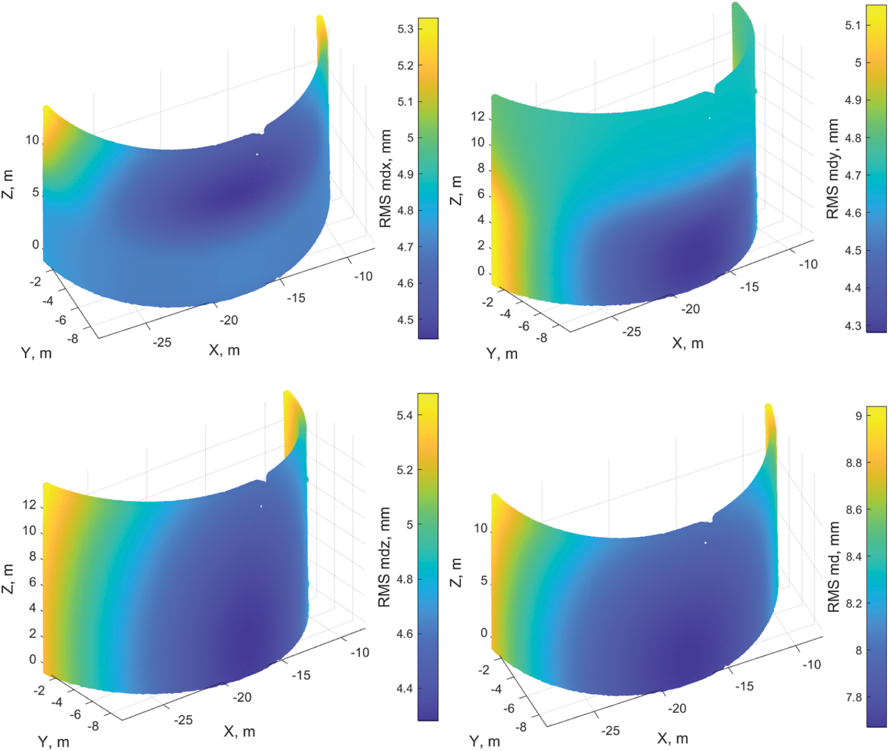
Figure 4: Distribution of accuracy in determining deformations on the tank’s surface along the coordinate axes and the accuracy in determining displacements in space
According to the modeling results, the maximum accuracy of determining spatial displacements is 9, and 7.4 mm for radial displacements. For a 95% confidence level and appropriate coefficient t = 2.5, the limit error in space is 22.5 mm, while the radial limit error is 18.4 mm. These values correspond to the limit accuracy. Therefore, any values exceeding these specified thresholds should be regarded as potential deformations. In the following subsection, this threshold will be used to distinguish measurement noise from possible deformations.
4.2 Deformation and Displacement Analysis by Cylinder Surface Simulation
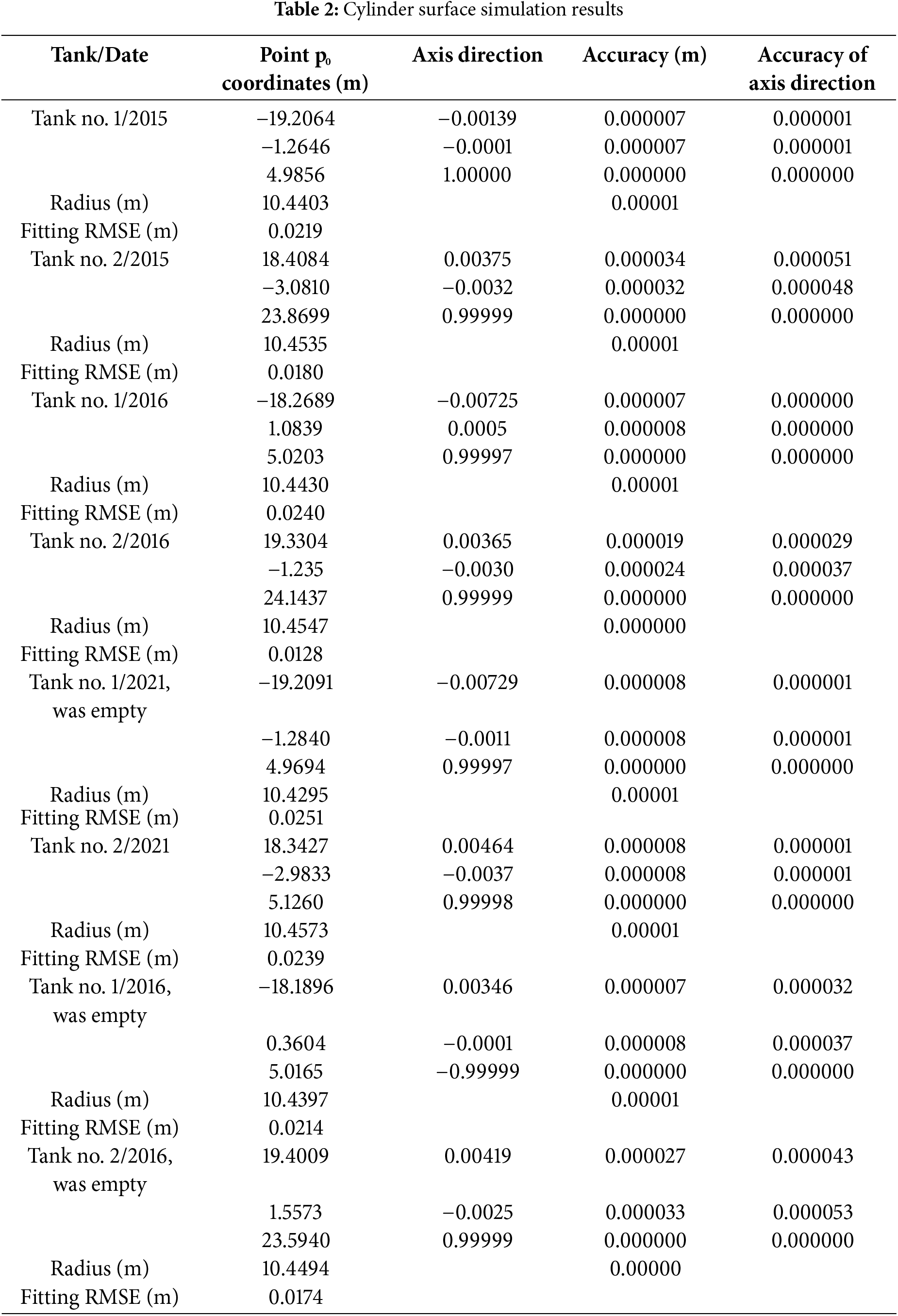
The oil tank surfaces were simulated using Eq. (9). For each point cloud, the cylinder parameters were estimated along with their accuracy estimations. The fitting procedure involved two steps. In the first step, the point cloud was fitted, and the RMSE was calculated. In the second step, the outlier exclusion rule was applied. All measurements with residuals greater than 2.5 times the RMSE were treated as blunders and removed from further processing. The filtered point cloud was fitted again with a cylindrical surface, and final estimations were determined. The quality of the fit was assessed using the RMSE. As the final output of the tank simulation, we provide estimations for the cylinder parameters along with their accuracy (Table 2).
The comprehensive information on approximation quality includes a residual histogram and a correlation matrix. In Fig. 5, the histograms are displayed alongside a theoretical curve (in red) which represents a normal distribution curve based on estimations derived from the fitting procedure.
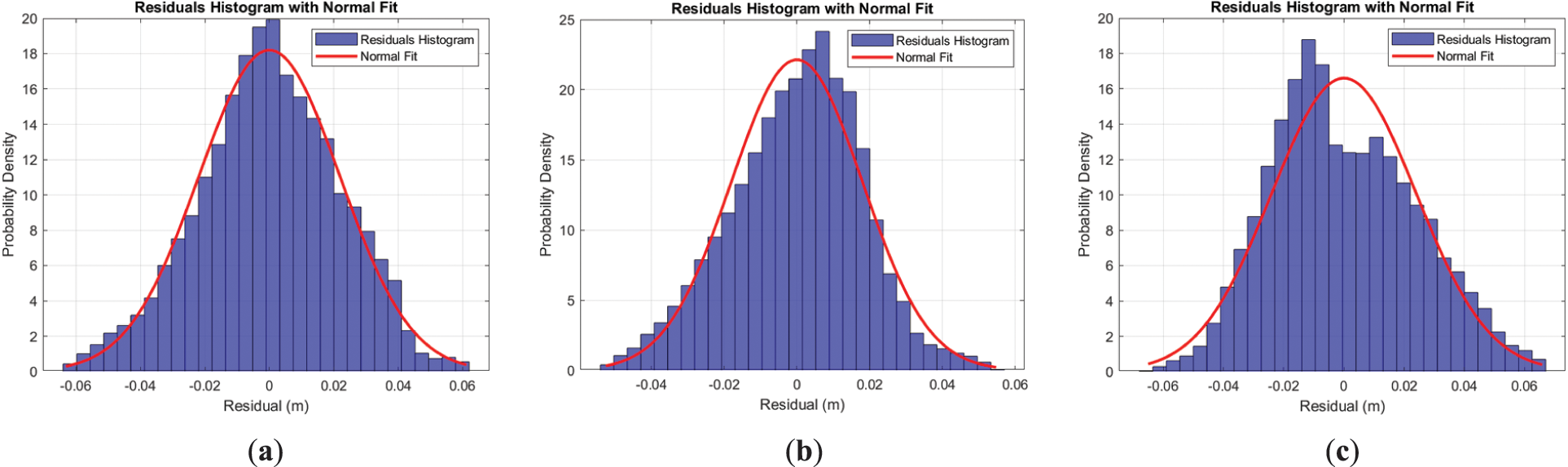
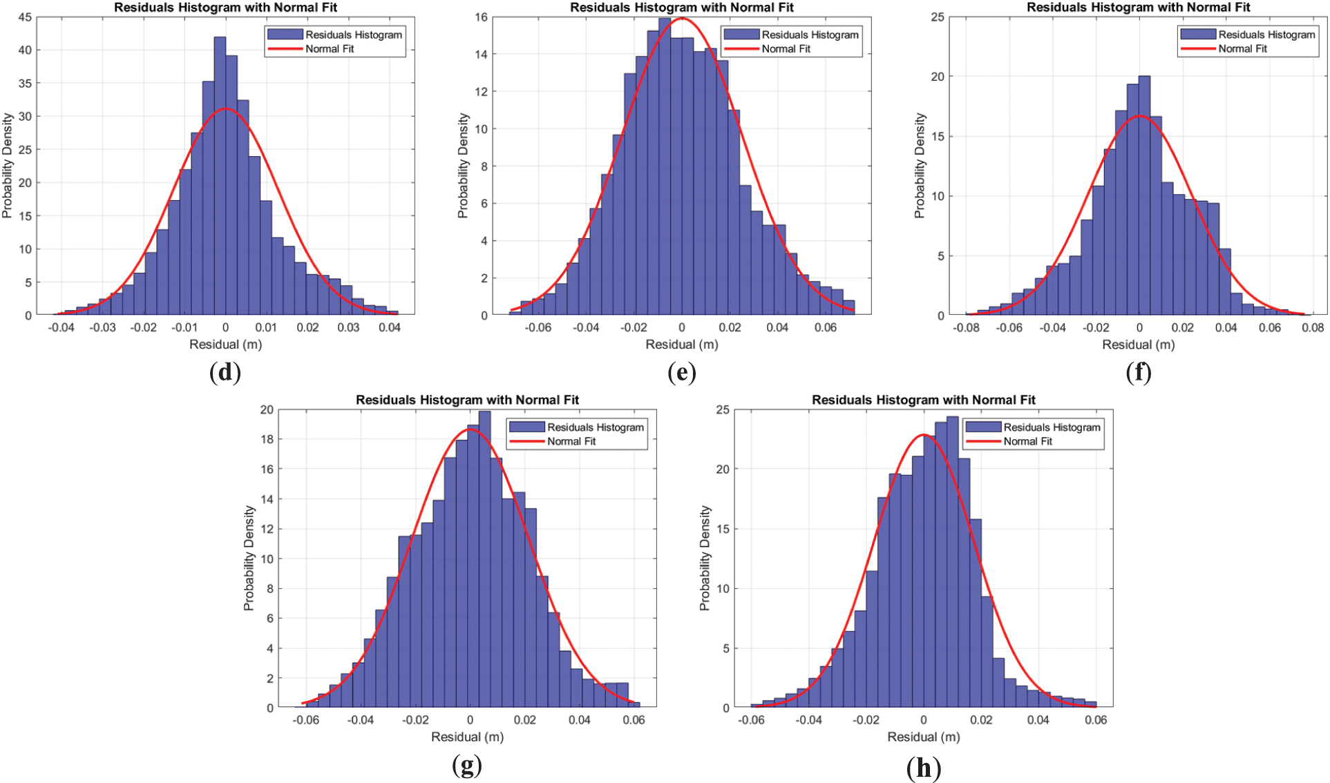
Figure 5: Histograms of residual distribution: (a) Tank No. 1/2015; (b) Tank No. 2/2015; (c) Tank No. 1/2016; (d) Tank No. 2/2016; (e) Tank No. 1/2021, empty; (f) Tank No. 2/2021; (g) Tank No. 1/2016, empty; (h) Tank No. 2/2016, empty
Despite some deviations in the histograms, they primarily conform to a normal distribution curve. The structure of the correlation matrix, along with the correlation coefficients and the covariance matrix, remains consistent across observation epochs for both tanks. The coefficient values fluctuate within an expected range of measurement accuracy. A sample of the covariance and correlation matrix is provided in Fig. 6.
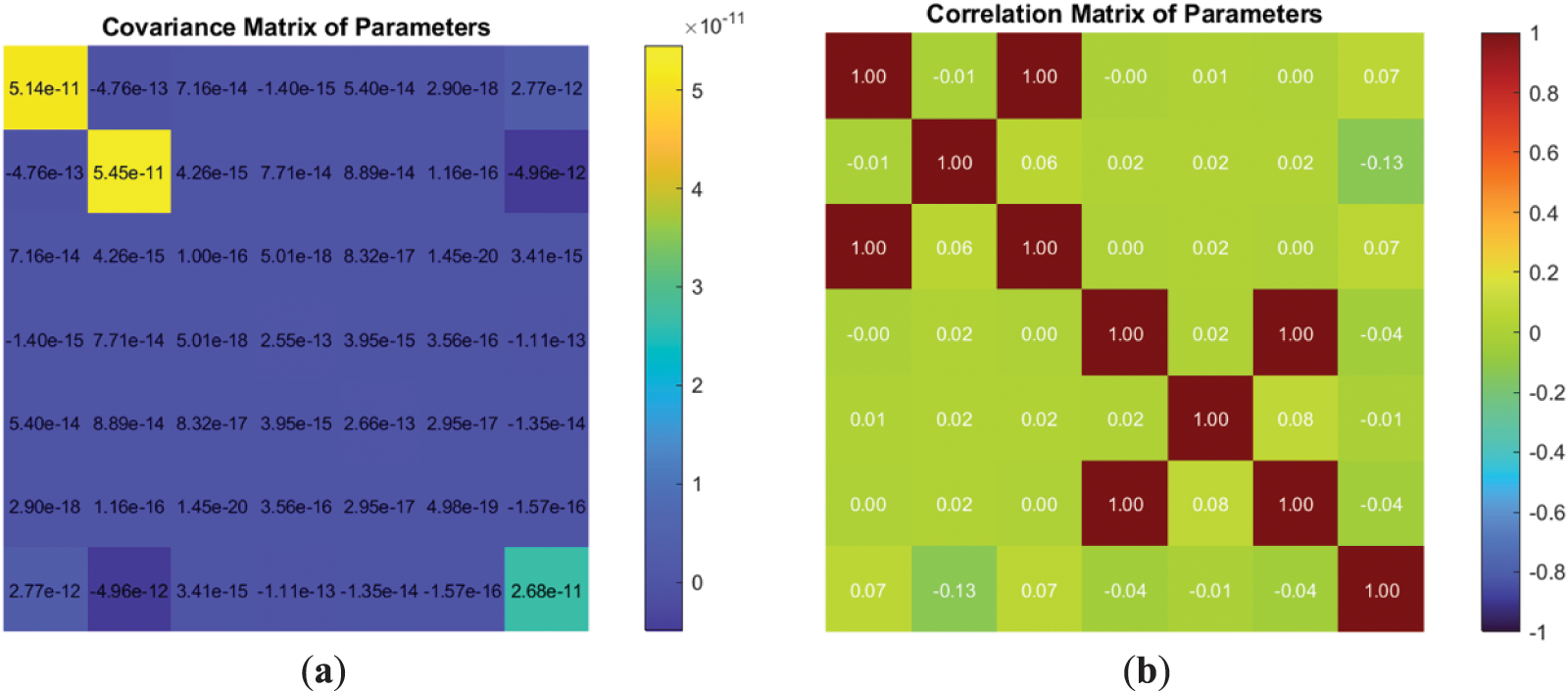
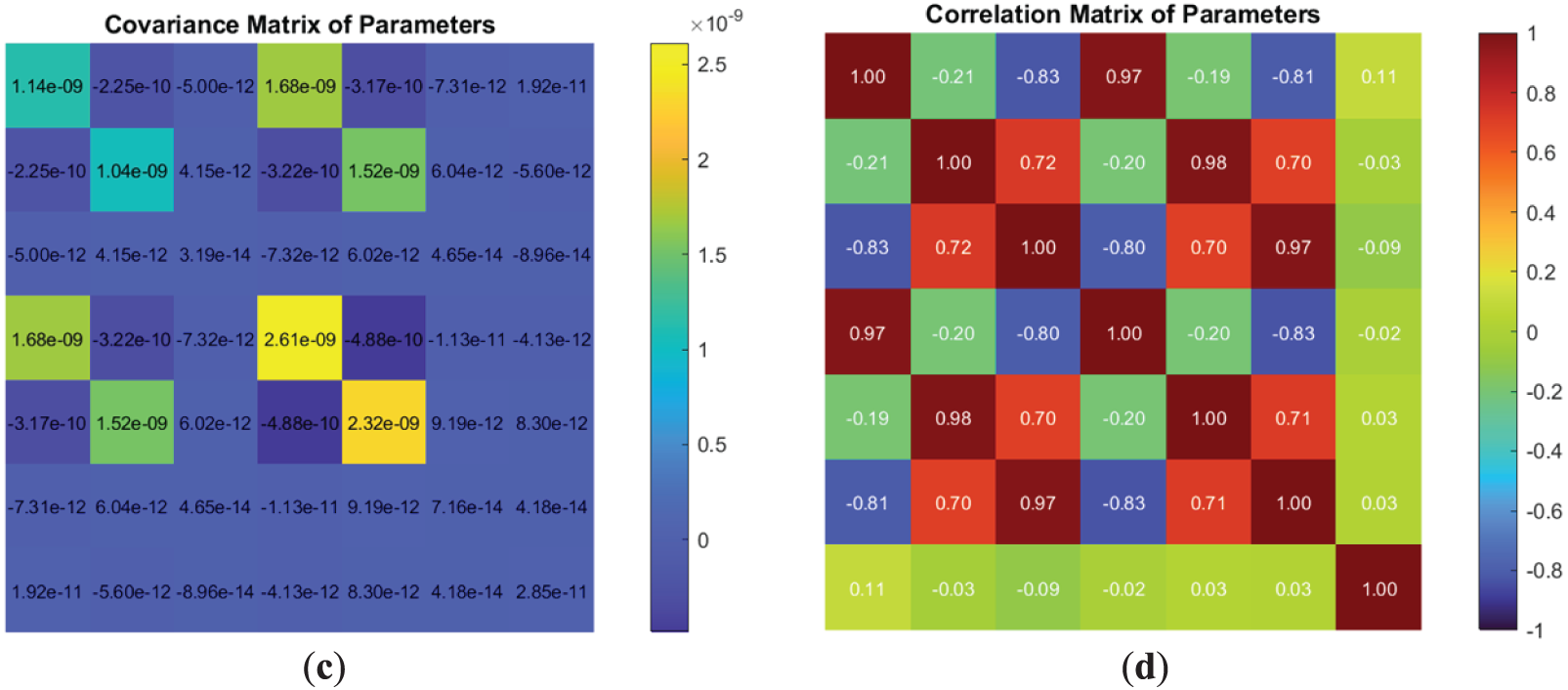
Figure 6: Structure and elements of covariance and correlation matrix: (a) Structure of the covariance matrix of the estimated parameters for Tank No. 1/2015; (b) Structure of the correlation matrix of the estimated parameters for Tank No. 1/2015; (c) Structure of the covariance matrix of the estimated parameters for Tank No. 2/2015; (d) Structure of the correlation matrix of the estimated parameters for Tank No. 2/2015
The correlation between estimated parameters is very strong, especially for Tank No. 2. However, in the case of significant data redundancy, local variations in measurements will not affect parameter estimation.
Diagrams illustrating the residuals of the point cloud from the best-fitted cylinder were created based on the estimated parameters (Fig. 7).
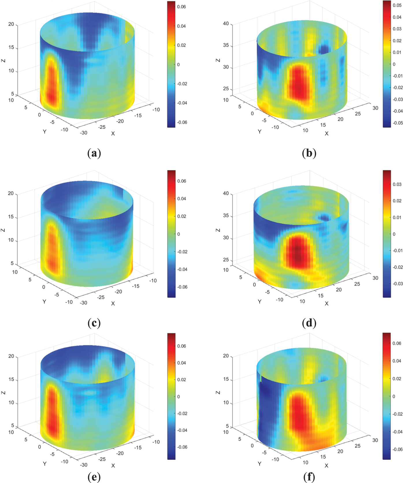
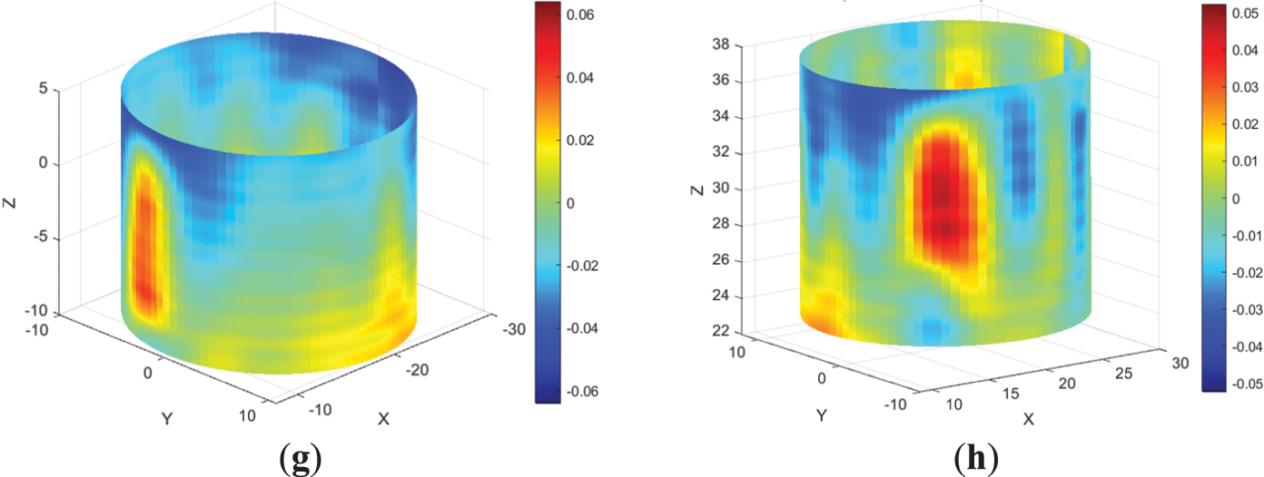
Figure 7: Residual fields regarding the optimal cylinder surface (all dimensions are in meters): (a) Tank No. 1/2015; (b) Tank No. 2/2015; (c) Tank No. 1/2016; (d) Tank No. 2/2016; (e) Tank No. 1/2021, empty; (f) Tank No. 2/2021; (g) Tank No. 1/2016, empty; (h) Tank No. 2/2016, empty
Before we embark on the deformation and displacement analysis, it would be wise to analyze the obtained parameters and their associated accuracy. The residuals analysis shows a normal distribution centered around zero, suggesting no reason for significant systematic errors. The RMSE ranges from 0.0128 to 0.0251 m, which is less than or slightly exceeds the critical value specified in Section 4.1. Due to the considerable data redundancy, the coordinates of point p0 and the axis direction are estimated with high reliability, allowing us to use these estimated values with confidence for further analysis.
The residuals in Fig. 7a,b, obtained during the first observation epoch, illustrate the deviations of the actual tank surface from the best-fitted cylinder. The visual comparison of residuals reveals no deformations between observation epochs. The differencing procedure for various epochs indicates that the detected deformations of the tank surface remain below the critical value of 18.4 mm. Thus, these values should be treated as random errors. For both oil tanks, their shape remains unchanged. The deviations observed in Fig. 7a,b likely represent inherent construction errors, as they have the same value and remain stable over time.
Let us compare the fitting results for the same observation epoch under different tank loads. Fig. 7g,h illustrate the residuals for empty tanks. By comparing Fig. 7a,b with Fig. 7g,h, we can conclude that there are no significant deformations. However, the analysis of the radius estimations in Table 1 provides some additional insights. For tank No. 1, the difference in cylinder radius before tank filling is
The cylinder surface represents the point cloud as a whole. To understand the potential variations in oil tank radius and respective conicity, we must construct cross-sections and estimate the local circle parameters for these sections. Furthermore, the cross-sections allow us to identify the geometric changes for both full and empty tanks. Each tank was examined using thirteen cross-sections, each 10 cm wide, resulting in an average of 100,000 to 150,000 points per section. The results of the 3D circle fitting are presented in Table 3.
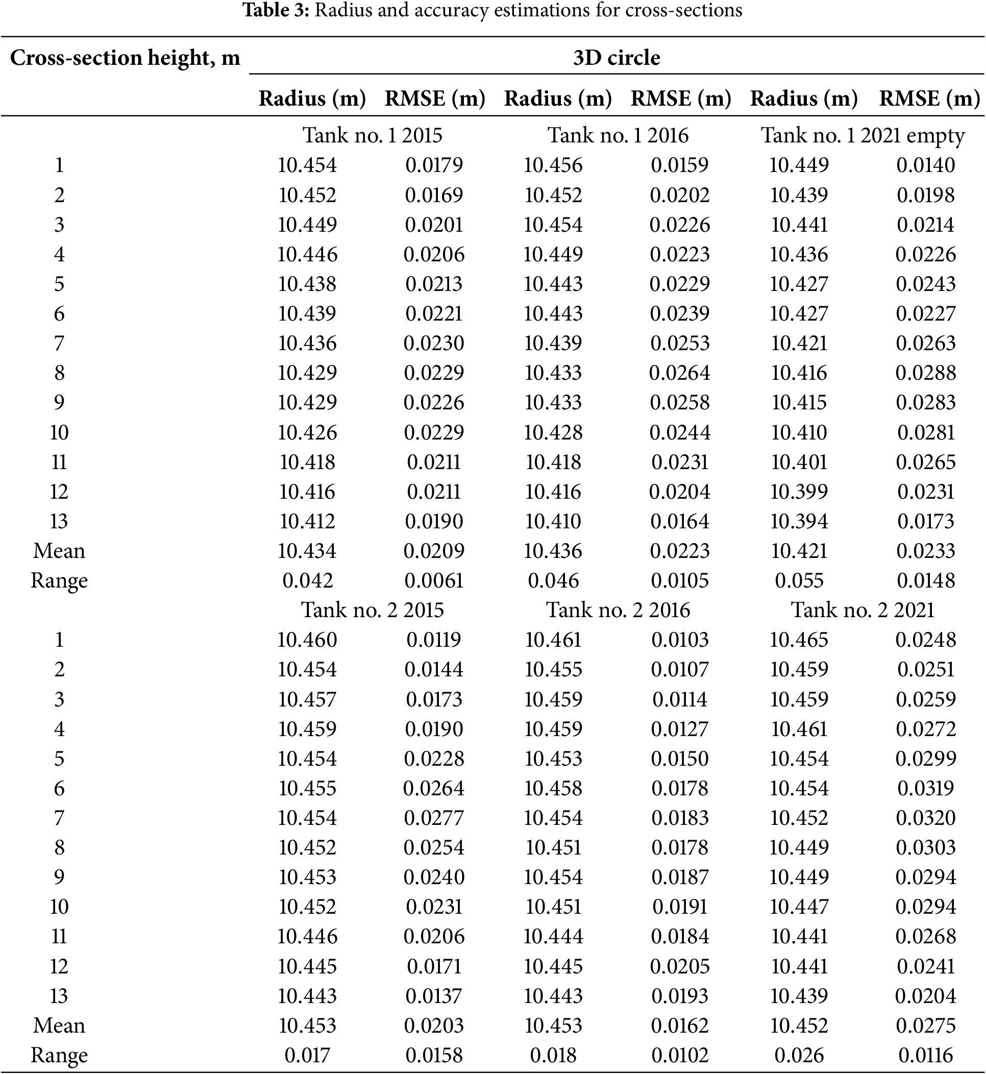
The analysis of Table 3 is intricate. Therefore, we present the cross-section fitting results in charts (Fig. 8), which illustrate the changes in radius based on cross-section height and trends in fitting RMSE.
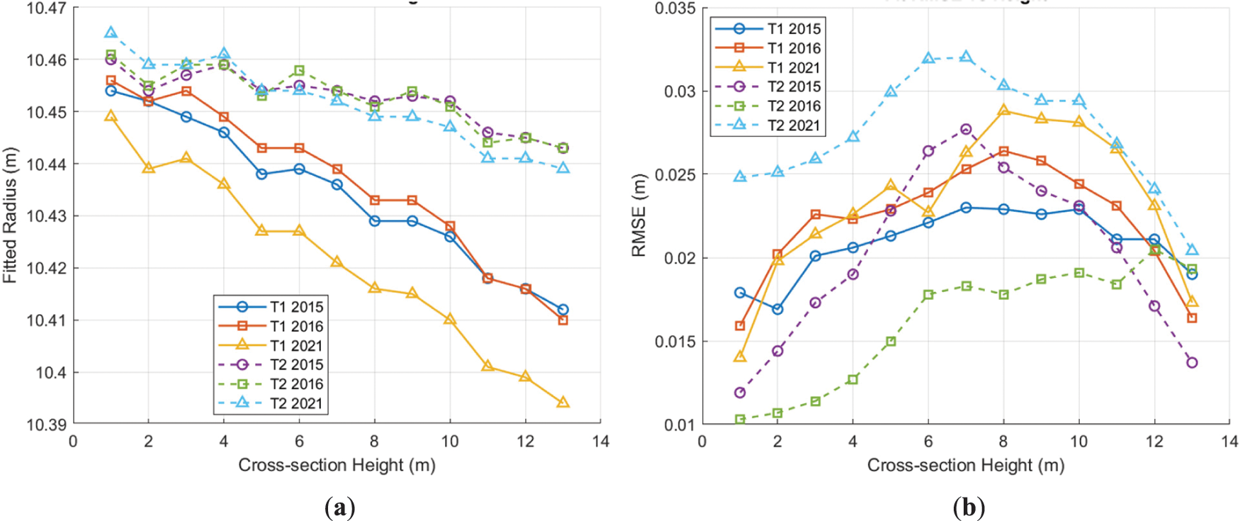
Figure 8: Radius analysis in cross-sections: (a) Estimated radius values for different cross-sections; (b) RMSE for different cross-sections
The results in Table 3 and Fig. 8 reveal intriguing findings that are not evident from cylinder fitting alone. The overall picture emerging from Fig. 8a indicates that both tanks have a slightly conical shape rather than a purely cylindrical one. The radius decreases from the bottom to the top by 48 mm for tank No. 1 and by 20 mm for tank No. 2. Additionally, Fig. 8a illustrates the radius change for the empty tank No. 1. The likely cause of this change is environmental load, particularly temperature variation. Another noteworthy finding is that fitting accuracy depends on the cross-section height. A more precise analysis for both full and empty tanks can be conducted using scanning data obtained under the same surveying conditions. The results of cross-section fitting are presented in Table 4.
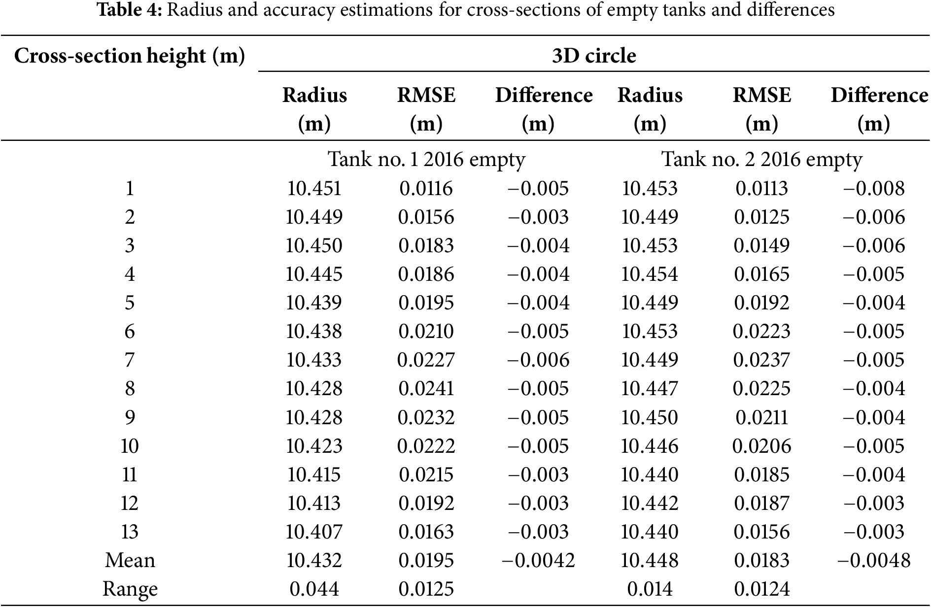
One can observe that the estimates for the radius differences between full and empty tanks closely align with those obtained from cylinder fitting. The provided data (Table 4) are consistent with previous findings, indicating a slight conicity that must be taken into account for precise simulation.
The final step is to determine the oil tank displacement. As the total movement of an oil tank is minimized, the primary displacement is expected to occur as an inclination. We used the estimated cylinder parameters from Table 1 to calculate this inclination and established the angles between the two vectors using Rodrigues’ formula. The resulting inclinations are presented in Table 5. For convenience, the inclinations expressed in degrees were converted to millimeters for more straightforward interpretation.
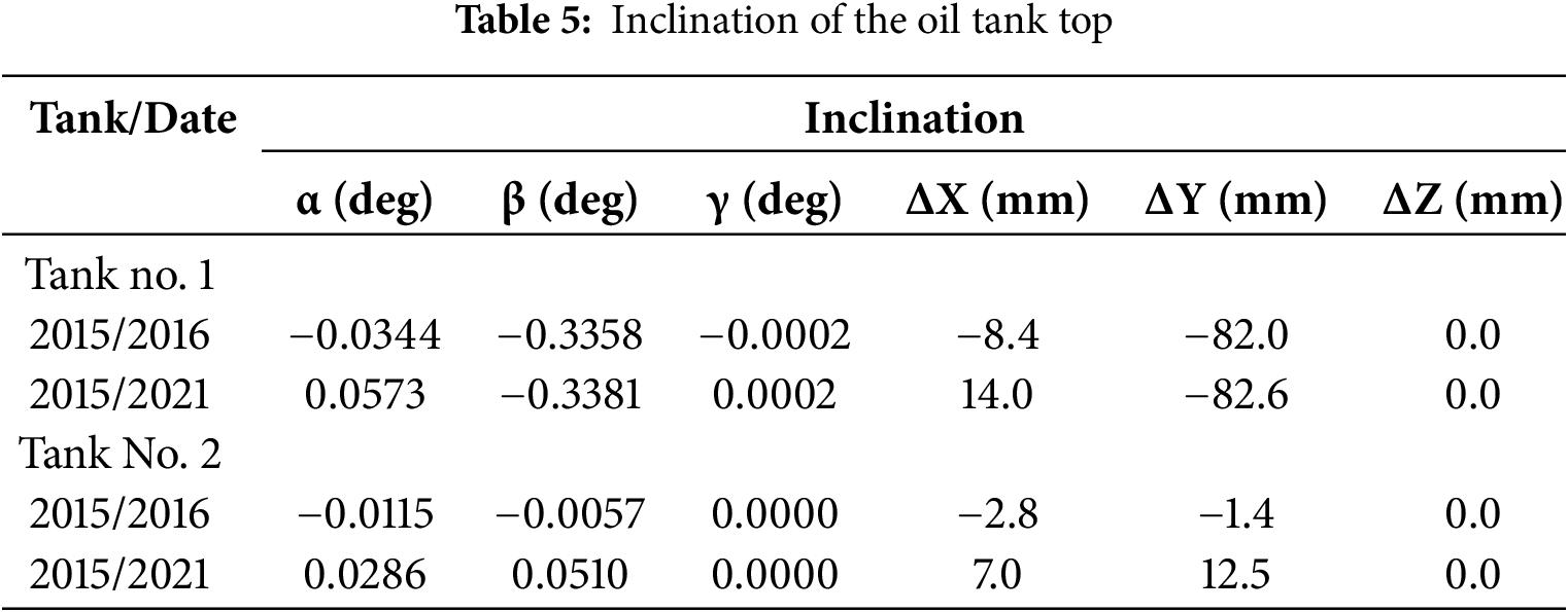
The results in Table 3 indicate that the inclination along the Y-axis for tank No. 1 has a significant magnitude of approximately −82 mm, which remains stable over the next five years. Therefore, the initial inclination is stabilized and poses no critical threats to further exploitation. The inclinations along the other axis and for tank No. 2 can be considered negligible. Overall, our study has shown that oil tanks remain stable despite minor surface deformations. Specifically, oil tank No. 1 experienced an inclination along the Y-axis. For the final analysis, we gathered all findings related to deformations and displacements and forwarded them for FEM analysis.
The multi-level deformation analysis, including cylinder fitting, cross-section analysis, and inclination estimation, yields a consistent conclusion regarding the behavior of the oil tanks. The cylinder fitting results demonstrate high stability over time, with RMSE values between 12.8 and 25.1 mm. These values are well within the previously assigned limit error of 18.4 mm for radial deformation. These values suggest that no significant systematic deformations occurred during the observation period. Moreover, the residuals follow a near-normal distribution, indicating that deviations are predominantly stochastic. Further insights emerge from the cross-sectional analysis, which reveals a consistent decrease in tank radius from bottom to top. The detected changes, 48 mm for Tank No. 1 and 20 mm for Tank No. 2, suggest a slight conicity. Such a shape is likely due to initial construction imperfection or long-term operational effects such as pressure or temperature cycles. The observed change in radius between full and empty tanks (~4–5 mm) also supports the presence of minor elastic deformation due to internal pressure, which remains within safe and expected limits. The analysis of empty tank cross-sections presented in Table 4 shows radius variations between full and empty states within the range of −3 to −6 mm, aligning closely with the differences observed in cylinder fitting results.
Regarding tank inclination, Table 5 identifies a significant and stable inclination for Tank No. 1 along the Y-axis, estimated at approximately −82 mm, corresponding to a tilt angle of −0.3358°. This inclination remains unchanged over multiple observation epochs. It proves its origin is likely related to construction or assembling works. In contrast, Tank No. 2 has only a negligible inclination, confirming its stability.
In summary, all evaluated deformations and displacements remain within the defined safety tolerances. The identified deformations are either random and static, such as tank inclination, or temporary and elastic, such as radius changes due to loading. These results strongly suggest the absence of progressive deformation over the observed years. However, the detection of tank conicity and measurable inclination highlights the need for such detailed multi-scale analyses in long-term structural monitoring. These findings provide a reliable base for further finite element modeling to assess structural integrity under simulated loads.
The goal of the FEM simulation is twofold: first, to validate the findings from our geometric analysis; second, to examine the stress-strain conditions of the deformed tanks caused by construction imperfections. For the simulation, SCAD Office software was used. A cylindrical tank with a wall of constant thickness was simulated as clamped to a flat bottom and subjected to a linearly distributed internal pressure from oil with a bulk density of 10 t/m3. For the simulation, the following parameters were accepted: modulus of elasticity E = 2.1 × 10⁸ kPa, Poisson’s ratio ν = 0.3, tank wall thickness t = 0.012 m, and tank height H = 15.0 m. The finite element model consists of 2190 four-node shell elements. The finite element mesh is divided in the meridional direction with a 10-degree step and in height with a 0.5 m step. Boundary conditions at the clamping level at the bottom are determined by imposing connections in all directions of angular and linear displacement. The number of nodes in the calculation scheme is 2170 (Fig. 9a).
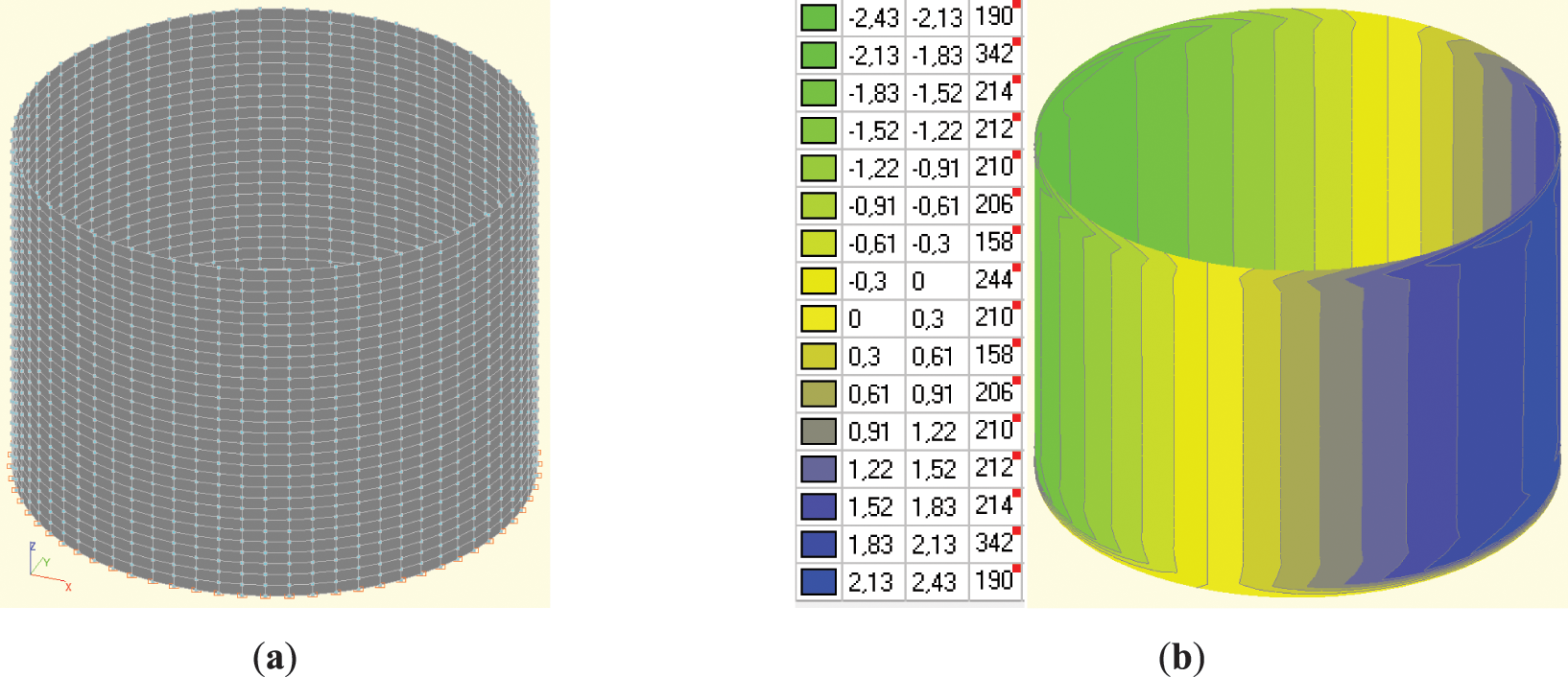
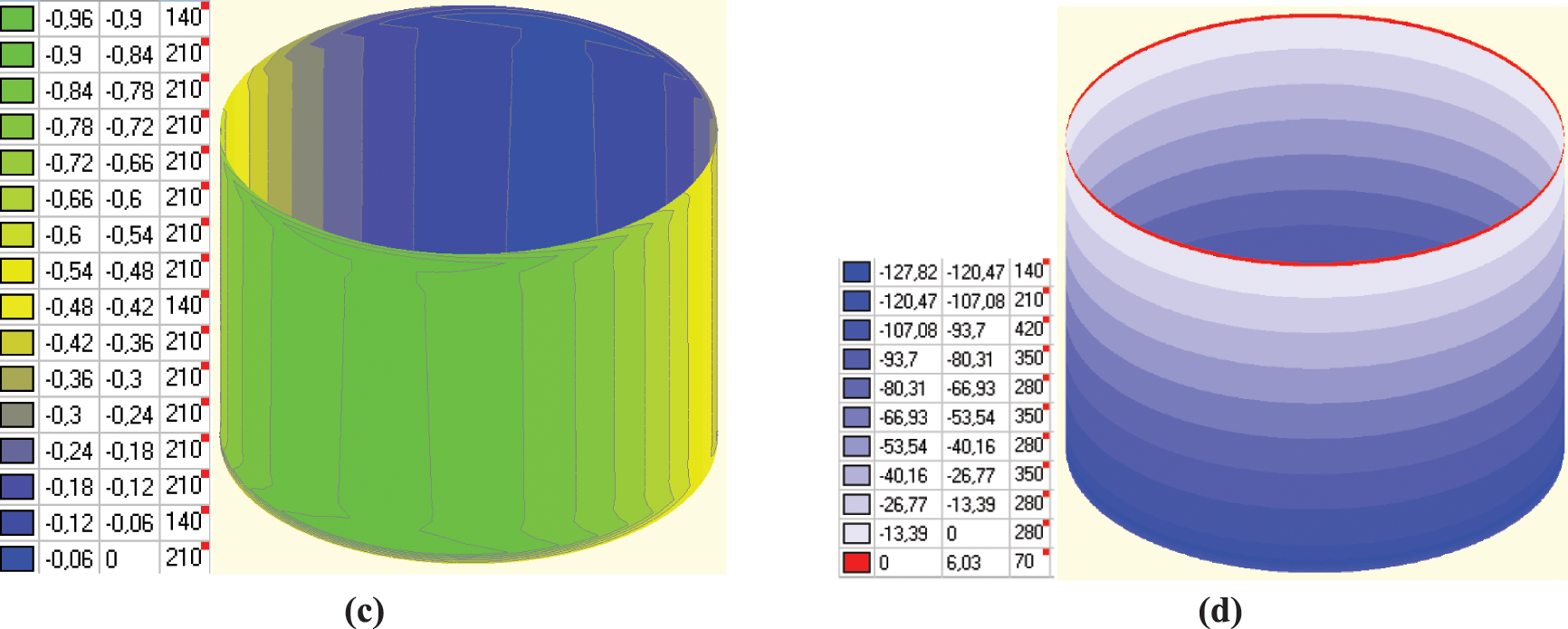
Figure 9: FEM simulation of ideal loaded tank: (a) Tank partitioning into rectangular finite elements; (b) Deformation diagram for X-axis in mm; (c) Deformation diagram for Y-axis in mm; (d) Stress field in tons/m2
Fig. 9b,c illustrate the distribution of deformations for the idealized case, where no external or internal loads are applied, and the tank surface remains undistorted. As shown, the total deformation in the radial direction reaches approximately 3 mm. This value is consistent with findings from studies on both full and empty tanks. Note that for results yielded by TLS, the average difference was around 4 mm in the radial direction. Thus, the measurement results and simulation demonstrate good correspondence.
Recall that for empty tank No. 1 in 2021, we observed a significant decrease in radius compared to the previous observation period. The premise was that variations in environmental temperature might have caused this difference. To test this hypothesis, the same tank was simulated under two temperature scenarios. The first simulation was conducted at the standard temperature of +10°C (Fig. 10a,b) and under winter conditions of −20°C (Fig. 10c,d). The simulation results are presented in Fig. 10a–d.
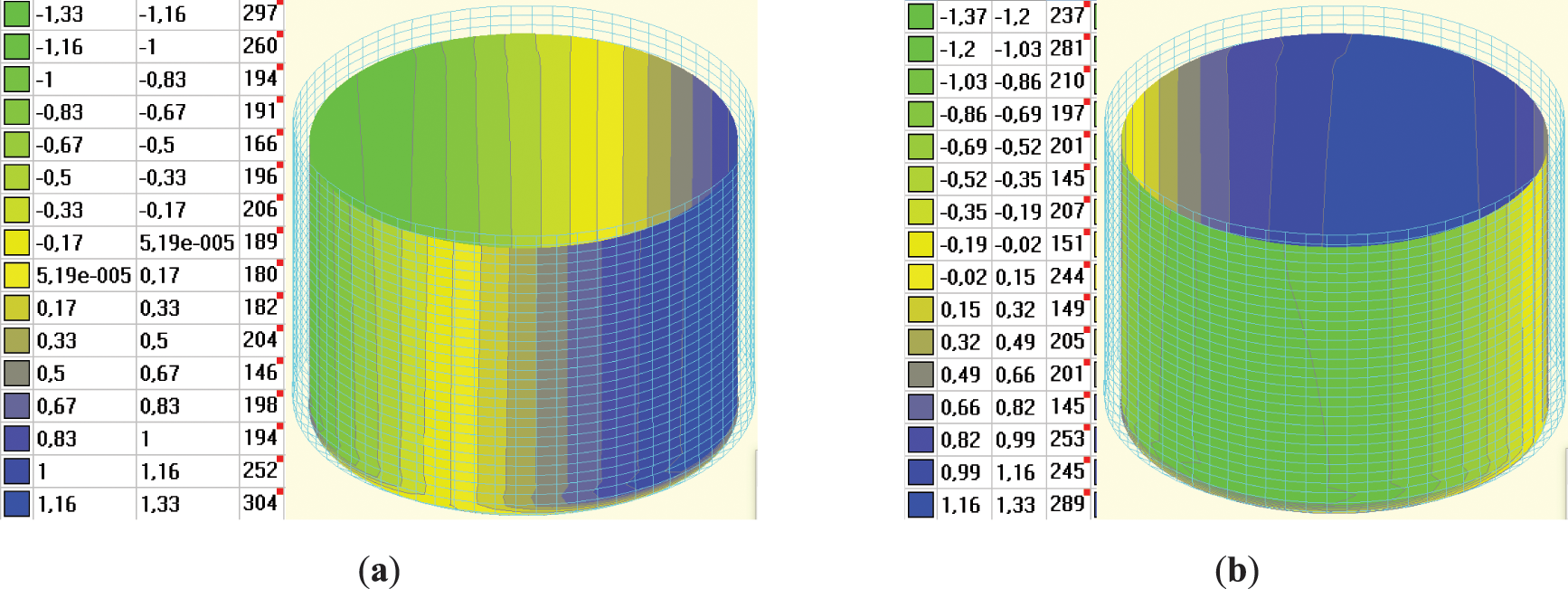
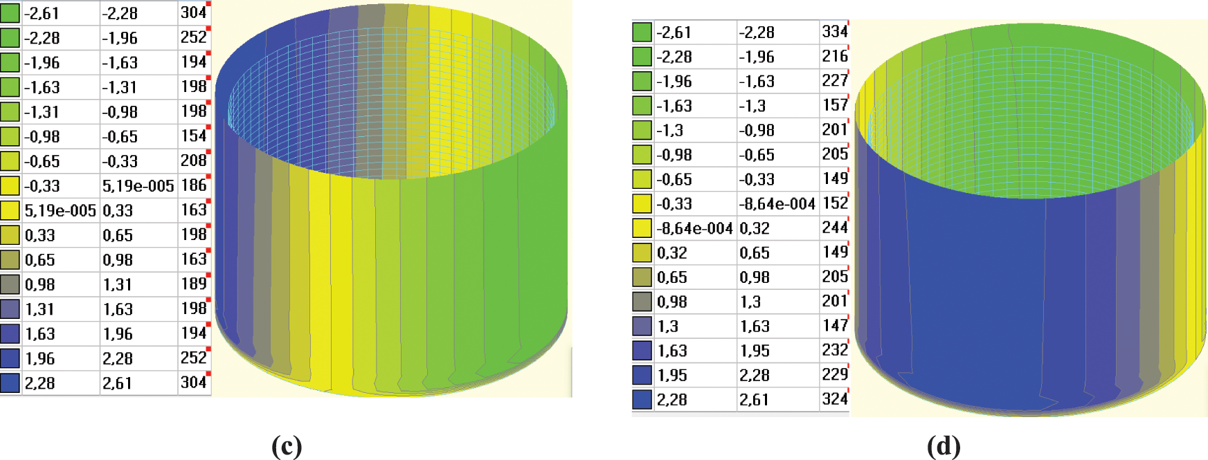
Figure 10: FEM simulation of ideal empty tanks for different temperatures: (a) Deformation diagram for t = +10°C for X-axis in mm; (b) Deformation diagram for t = +10°C for Y-axis in mm; (c) Deformation diagram for t = −20°C for X-axis in mm; (d) Deformation diagram for t = −20°C for Y-axis in mm
In summary, temperature deformation occurred, but its magnitude does not exceed 4 mm in the radial direction. This value must be considered for monitoring data analysis. However, the value of this deformation is insufficient to explain the nearly 20 mm difference in radius observed between 2015 and 2021. Therefore, this phenomenon will be the subject of future studies.
Finally, we examined how the identified construction flaws could affect the future use of oil tanks. As a case study, we presented the FEM simulation of the fully loaded oil tank No. 1 (Fig. 11).
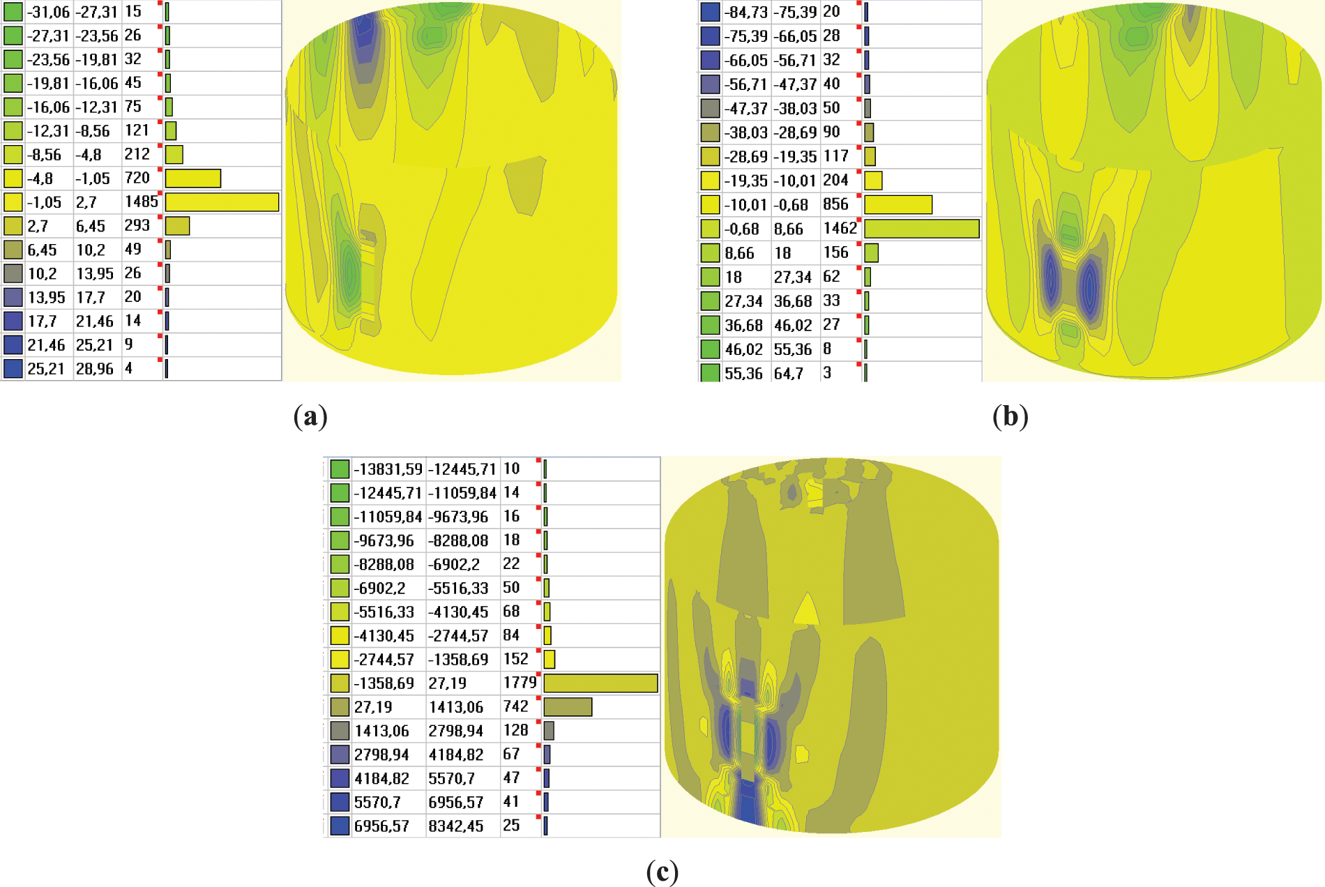
Figure 11: FEM simulation of real tank No. 1: (a) Deformation diagram for X-axis in mm; (b) Deformation diagram for Y-axis in mm; (c) Stress field in tons/m2
The monitoring revealed alternating bulging patterns along the tank shell surface, ranging from −0.06 to +0.06 m, due to errors in fabrication and installation. The simulations show reliable agreement between the results when accounting for the geometric nonlinearity, demonstrating good correspondence between the calculated values and those obtained through monitoring. In the FEM analysis, the results are as follows: σ = 166 MPa (which does not exceed the calculated strength of steel); the oscillation frequency is 0.13 s−1; the horizontal oscillation amplitude is 9 mm; and the deformation range is 0.08 m. Since the calculation results are free from the errors inherent in field geodetic work, the discrepancies can be considered acceptable. If the tanks were welded into a perfect round shape, wall deformations would be negligible (up to 2 mm, see Fig. 9) because the radial vectors acting on the tank would be entirely identical. The stresses and deformations are uniformly distributed across the entire circumference. Significant stress distortions occur in these areas as soon as geometric irregularity appears due to construction flaws (within 3–5 cm). Consequently, non-uniform wall deformations (ranging from 30 to 80 mm) arise immediately. Results in Section 4.2 suggest that deviations such as conicity or radius reduction may result from loading and environmental conditions. FEM simulation confirms that such deformations are physically plausible and align with material properties and stress-strain mechanics. However, the FEM also indicates that temperature alone cannot explain the larger variation (20 mm) seen between 2015 and 2021, pointing to the need for further study. Therefore, monitoring is an indispensable process to support further safe exploitation.
Returning to the questions posed at the beginning of this study, it is now possible to state that TLS can serve as an effective tool for oil tank monitoring. This conclusion is supported by the developed method for estimating TLS accuracy. The accuracy simulation under standard scanning conditions has demonstrated the capability to estimate accuracy and detect tank surface deformations greater than 18 mm. The data processing strategy is crucial. This study introduced a new processing approach based on the cylinder fitting algorithm. A key strength of the current algorithm is its ability to identify both surface deformations and tank displacements (inclinations). The cylinder fitting was complemented by cross-section analysis. The corresponding calculation workflows are outlined in the text. The suggested workflows were tested on two oil tanks, scanned three times in 2015, 2016, and 2021. Additionally, the tanks were scanned twice in 2016, once when empty and once when full. The goal was to evaluate the capabilities of TLS to detect geometric changes under different loads. TLS analysis demonstrated that:
- Both oil tanks show local deformations of up to 60 mm due to construction defects, which remain stable throughout the monitoring period.
- The surface deformations for both tanks remain within allowable limits and show radial components of less than 15 mm over six years.
- The study of surface deformations in the empty state revealed a tank radius contraction of about 4 mm.
- For tank No. 1, the inclination along the Y-axis of 82 mm was detected, while tank No. 2 shows a negligible inclination.
- Cross-section analysis confirmed the radius changes for full and empty tank states.
- Cross-section analysis revealed that both tanks have a non-cylindrical shape, deviating toward a conical surface with a mean radius change from bottom to top.
The FEM analysis confirmed the observed relationship between radius changes in full and empty oil tanks. The deformations induced by temperature variations must be incorporated into the monitoring data analysis. However, their contribution to the overall deformation detected for tank No. 1 in 2021 is minor. FEM simulation suggests that potential deformation may progress due to imperfections in tank construction. In a full oil tank, localized deformations can propagate across the shell, creating additional stress concentrations. Therefore, further monitoring is recommended.
This investigation will serve as a base for future studies of oil tanks. The methods developed in this research may also be applied to other structures with similar geometries, such as cooling towers, chimneys, etc. Future studies will have to focus on investigating ellipticity. This can be approached in two ways: by fitting an elliptical cylinder or by fitting 3D ellipses to cross-sections. The second research direction involves analyzing the detected conicity of the tank. Therefore, an algorithm and workflow should be developed for cone fitting and subsequent analysis of this surface.
Acknowledgement: Not applicable.
Funding Statement: The authors received no specific funding for this study.
Author Contributions: The authors confirm contribution to the paper as follows: Conceptualization, Roman Shults and Oleksandr Adamenko; software, Roman Shults and Andriy Annenkov; validation, Roman Shults, Oleksandr Adamenko and Andriy Annenkov; formal analysis, Roman Shults and Natalia Kulichenko; investigation, Roman Shults, Andriy Annenkov and Natalia Kulichenko; resources, Oleksandr Adamenko; data curation, Oleksandr Adamenko; writing—original draft preparation, Andriy Annenkov and Natalia Kulichenko; writing—review and editing, Roman Shults; visualization, Roman Shults, Andriy Annenkov and Natalia Kulichenko; supervision, Roman Shults; project administration, Roman Shults; funding acquisition, Roman Shults. All authors reviewed the results and approved the final version of the manuscript.
Availability of Data and Materials: The data that support the findings of this study are available from the corresponding author, Roman Shults, upon reasonable request.
Ethics Approval: Not applicable.
Conflicts of Interest: The authors declare no conflicts of interest to report regarding the present study.
Abbreviations
| RMSE | Root Mean Square Error |
| TLS | Terrestrial Laser Scanning |
| FEM | Finite Element Method |
References
1. Savvaidis P. Long term geodetic monitoring of the deformation of a liquid storage tank founded on piles. In: Proceedings of 11th FIG Symposium on Deformation Measurements; 2003 May 25–28; Santorini, Greece. [Google Scholar]
2. Cosarcă C, Sărăcin A, Savu A, Florentin A, Negrilă C. Monitoring the deformation of an industrial tank in the discharge and filling process. J Geodesy Cartograp Cadastre. 2019;10:55–9. [Google Scholar]
3. Toś C. Importance of geodetic surveys in terms of assembly and operation safety on external tendon-stressed tanks. Tech Trans Environ Eng. 2014;20(1-Ś):53–63. [Google Scholar]
4. Erdenenemekh G. Determine of losses storage tank by geodetic measurements. Earth Sci. 2023;12(5):116–20. doi:10.11648/j.earth.20231205.11. [Google Scholar] [CrossRef]
5. Shults R. Geospatial monitoring of engineering structures as a part of BIM. Int Arch Photogramm Remote Sens Spat Inf Sci. 2022;46(5/W1-2022):225–30. doi:10.5194/isprs-archives-XLVI-5-W1-2022-225-2022. [Google Scholar] [CrossRef]
6. Gairns C. Development of semi-automated system for structural deformation monitoring using a reflectorless total station [master’s thesis]. Saint John, NB, Canada: University of New Brunswick; 2008. [Google Scholar]
7. Beshr AAA. Monitoring the structural deformation of tanks. Saarland, Germany: LAP LAMBERT Academic Publishing; 2012. [cited 2025 Mar 20]. Available from: https://www.researchgate.net/publication/280297590_Monitoring_the_structural_deformation_of_tanks. [Google Scholar]
8. Delčev SŠA, Ogrizović V, Gučević J. Geodetic method of the fuel tank form inspection. Measurement. 2012;45:2376–81. doi:10.1016/j.measurement.2011.10.003. [Google Scholar] [CrossRef]
9. Burak K, Kovtun V, Nychvyd M. Building 3D surfaces of land storage vertical cylindrical steel tank using bicubic spline interpolation. Geodesy Cartogr. 2019;45(2):85–91. doi:10.3846/gac.2019.6301. [Google Scholar] [CrossRef]
10. Glowacki T, Grzempowski P, Sudol E, Wajs J, Zajac M. The assessment of the application of terrestrial Laser scanning for measuring the geometrics of cooling tower. Geomatics Landmanage Landsc. 2016;4:49–57. doi:10.15576/GLL/2016.4.49. [Google Scholar] [CrossRef]
11. Beshr AAA, Basha AM, El-Madany SA, El-Azeem FA. Deformation of high rise cooling tower through projection of coordinates resulted from terrestrial laser scanner observations onto a vertical plane. ISPRS Int J Geo Inf. 2023;12(10):417. doi:10.3390/ijgi12100417. [Google Scholar] [CrossRef]
12. Hamzić A, Kulo N, Đidelija M, Topoljak J, Mulahusić A, Tuno N, et al. Assessment of minaret inclination and structural capacity using terrestrial laser scanning and 3D numerical modeling: a case study of the Bjelave Mosque. Geomatics. 2025;5(1):8. doi:10.3390/geomatics5010008. [Google Scholar] [CrossRef]
13. Korumaz M, Betti M, Conti A, Tucci G, Bartoli G, Bonora V, et al. An integrated Terrestrial Laser Scanner (TLSDeviation Analysis (DA) and Finite Element (FE) approach for health assessment of historical structures. A minaret case study. Eng Struct. 2017;153:224–38. doi:10.1016/j.engstruct.2017.10.026. [Google Scholar] [CrossRef]
14. Alsadik B, Abdulateef NA, Khalaf YH. Out of plumb assessment for cylindrical-like minaret structures using geometric primitives fitting. ISPRS Int J Geo Inf. 2019;8(2):64. doi:10.3390/ijgi8020064. [Google Scholar] [CrossRef]
15. Canto L, de Seixas A. Geodetic monitoring on onshore wind towers: analysis of vertical and horizontal movements and tower tilt. Struct Monit Maint. 2021;8(4):309–28. doi:10.12989/smm.2021.8.4.309. [Google Scholar] [CrossRef]
16. Marjetič A. TPS and TLS laser scanning for measuring the inclination of tall chimneys. Geodetski Glasnik. 2018;49(49):29–43. doi:10.58817/2233-1786.2018.52.49.29. [Google Scholar] [CrossRef]
17. Beshr AAA. Determining the geometric parameters of circular cross section structures from geodetic observations. In: 4th International E-Conference on Advances in Engineering Technology and Management ICETM 2020 [Internet]. Online. [cited 2025 Mar 20]. Available from: https://www.researchgate.net/publication/348716608_Determining_the_geometric_parameters_of_circular_cross_section_structures_from_geodetic_observations. [Google Scholar]
18. Zeidan Z, Beshr AAA, Sameh S. Structural damage detection of elevated circular water tank and its supporting system using geodetic techniques. Geodesy Cartogr. 2020;69(1):117–40. doi:10.24425/gac.2020.131080. [Google Scholar] [CrossRef]
19. Hamzić A, Đidelija M, Topoljak J, Tuno N, Ambrožič T, Mulahusić A, et al. Inclination assessment of objects with circular base using algebraic circle fitting, linear regression, and bootstrapping. J Surv Eng. 2025;151(3):886. doi:10.1061/jsued2.sueng-1564. [Google Scholar] [CrossRef]
20. Hamzić A, Kamber Hamzić D, Avdagić Z. Rapid assessment of the verticality of structural objects with a circular base. In: Ademović N, Mujčić E, Akšamija Z, Kevrić J, Avdaković S, Volić I, editors. Advanced technologies, systems, and applications. Vol. 316. Berlin/Heidelberg, Germany: Springer; 2021. doi:10.1007/978-3-030-90055-7_41. [Google Scholar] [CrossRef]
21. Shults R, Seitkazina G, Soltabayeva S. The features of sports complex ‘Sunkar’ monitoring by terrestrial laser scanning. Int Arch Photogramm Remote Sens Spat Inf Sci. 2023;48(5/W2-2023):105–10. doi:10.5194/isprs-archives-XLVIII-5-W2-2023-105-2023. [Google Scholar] [CrossRef]
22. Harmening C, Hobmaier C, Neuner H. Laser scanner-based deformation analysis using approximating B-Spline Surfaces. Remote Sens. 2021;13(18):3551. doi:10.3390/rs13183551. [Google Scholar] [CrossRef]
23. Yanga H, Omidalizarandi M, Xu X, Neumann I. Terrestrial laser scanning technology for deformation monitoring and surface modeling of arch structures. Compos Struct. 2017;169:173–9. doi:10.1016/j.compstruct.2016.10.095. [Google Scholar] [CrossRef]
24. Akca D. Least squares matching of 3D surfaces. In: Proceedings of the 4th Symposium of Turkish Society for Photogrammetry and Remote Sensing; 2007 Jun 5–7; Istanbul, Turkey. [Google Scholar]
25. Shakarji CM. Least-squares fitting algorithms of the NIST algorithm testing system. J Res Natl Inst Stand Technol. 1998;103(6):633–41. [Google Scholar] [PubMed]
26. Koci J, Panou G. Techniques for least-squares fitting of curves and surfaces to a large set of points. J Surv Eng. 2025;151(2):81. doi:10.1061/jsued2.sueng-1552. [Google Scholar] [CrossRef]
27. Ferenc T, Gierasimczyk R, Mikulski T. Stress assessment of a steel bullet LPG tank under differential settlement based on geodetic measurements and sensitivity analysis. Pol Marit Res. 2024;4(124):122–30. doi:10.2478/pomr-2024-0056. [Google Scholar] [CrossRef]
28. Shults R, Soltabayeva S, Seitkazina G, Nukarbekova Z, Kucherenko O. Geospatial monitoring and structural mechanics models: a case study of sports structures. In: Proceedings of the 11th International Conference “Environmental Engineering”; 2020 May 21–22; Vilnius, Lithuania. p. 1–9. doi:10.3846/enviro.2020.685. [Google Scholar] [CrossRef]
29. Shults R, Roshchyn O. Preliminary determination of spatial geodetic monitoring accuracy for free station method. Geodetski List. 2016;70(4):355–70. Available from: https://hrcak.srce.hr/178883. [Google Scholar]
30. Rabbani T. Automatic reconstruction of industrial installations using point clouds and images [Ph.D. thesis]. Lahore, Pakistan: University of Engineering and Technology Lahore; 2006. [Google Scholar]
31. Dai JS. Euler-Rodrigues formula variations, quaternion conjugation and intrinsic connections. Mech Mach Theory. 2015;92:144–52. doi:10.1016/j.mechmachtheory.2015.03.004. [Google Scholar] [CrossRef]
32. Slabaugh GS. Computing euler angles from a rotation matrix. 2004 [Internet]. [cited 2025 Aug 13]. Available from: https://eecs.qmul.ac.uk/~gslabaugh/publications/euler.pdf. [Google Scholar]
Cite This Article
 Copyright © 2025 The Author(s). Published by Tech Science Press.
This work is licensed under a Creative Commons Attribution 4.0 International License , which permits unrestricted use, distribution, and reproduction in any medium, provided the original work is properly cited.
 Downloads
 Citation Tools