Ultrasonic Defect Localization Correction Method under the Influence of Non-Uniform Temperature Field

1  Introduction

During the service of high-temperature industrial components—such as nuclear power pipelines and turbine blades—ultrasonic non-destructive testing (NDT) [1] plays an irreplaceable role in structural health monitoring [2]. However, operation under elevated temperatures often gives rise to non-uniform thermal fields, leading to spatial variations in material properties such as elastic modulus and density, and consequently inducing spatial drift in ultrasonic wave velocity [3]. If defect localization is still calculated using the constant velocity [4] at room temperature, significant errors can occur, potentially resulting in missed or false detections of critical flaws and posing severe safety risks.

In recent years, extensive efforts have been made to investigate the influence of temperature on ultrasonic inspection. For example, Wu et al. [5] developed a frequency-domain model incorporating thermal effects and experimentally confirmed the pronounced increase in ultrasonic attenuation with temperature; Van De Wyer et al. [6] employed numerical ray-tracing to demonstrate that temperature alters propagation paths in liquid metals; Zhang et al. [7] established a velocity–temperature model for pipelines, highlighting the sensitivity of ultrasonic accuracy to thermal variations; Stevenson and Wang [8] experimentally validated correction factors in high-temperature carbon steel, showing reduced velocity and thickness measurement errors with rising temperature; and Liu et al. [9] proposed a signal-processing-based compensation strategy that markedly improved guided-wave stability in hot environments. Most of these studies, however, have concentrated on uniform thermal fields, leaving the spatial heterogeneity of velocity distributions under thermal gradients [10], and their coupled impact on defect localization [11], insufficiently understood. Furthermore, the nonlinear dependence of thermal properties such as thermal conductivity [12] and elastic modulus [13] on temperature is often oversimplified, thereby limiting both thermal-field modelling and velocity correction accuracy.

To address these challenges, we propose a defect-localization correction [14] framework that integrates multiphysics coupled modelling [15,16] with dynamic velocity tracking [17]. First, a two-dimensional thermo-acoustic model is constructed in COMSOL, where experimentally measured thermophysical parameters are used to define temperature-dependent material functions, yielding a velocity–temperature relationship [18] that captures the inherent nonlinearity. Second, to accommodate thermal gradients, a differential discretization approach is introduced: the steady-state heat conduction equation is solved numerically [19], the temperature of each differential segment is obtained, and the corresponding local velocity is computed to achieve cumulative correction. Numerical simulations demonstrate that this method effectively suppresses localization errors induced by thermal gradients, surpassing the limitations of traditional uniform-field correction schemes. The results provide a theoretical framework and technical pathway for enhancing the accuracy of ultrasonic inspection in high-temperature [20,21] and structurally complex environments.

2  Research Methodology

2.1 Overall Framework of the Defect Localization Correction Method

As illustrated in Fig. 1, the overall framework of the proposed defect localization correction method comprises four core components. First, multi-physics coupled modeling of heat conduction [22] and elastic wave propagation [23] is performed to capture the modulation of sound velocity distribution by the temperature field, which serves as the foundational context for all subsequent experiments. Second, the sound velocity–temperature relationship, c(T), is established by extracting travel times of ultrasonic echoes at different temperatures, thereby constructing a velocity correction model that supports defect localization in uniform temperature fields. Third, a gradient-varying temperature field model is developed, in which the temperature–position function T(y) is derived by incorporating the temperature-dependent thermal conductivity of the material; this provides the prerequisite for localization correction under non-uniform temperature conditions. Finally, correction pathways are determined according to the thermal environment: in uniform temperature fields, defect localization is directly corrected using the temperature-dependent sound velocity, whereas in non-uniform fields, the velocity field function c(y) is obtained by coupling c(T) with T(y), and dynamic correction of defect localization is achieved via the microelement integration method. This methodological framework establishes a complete chain from physical modeling [24] and parameter extraction to correction application, effectively mitigating the adverse impact of temperature gradients on ultrasonic inspection accuracy.

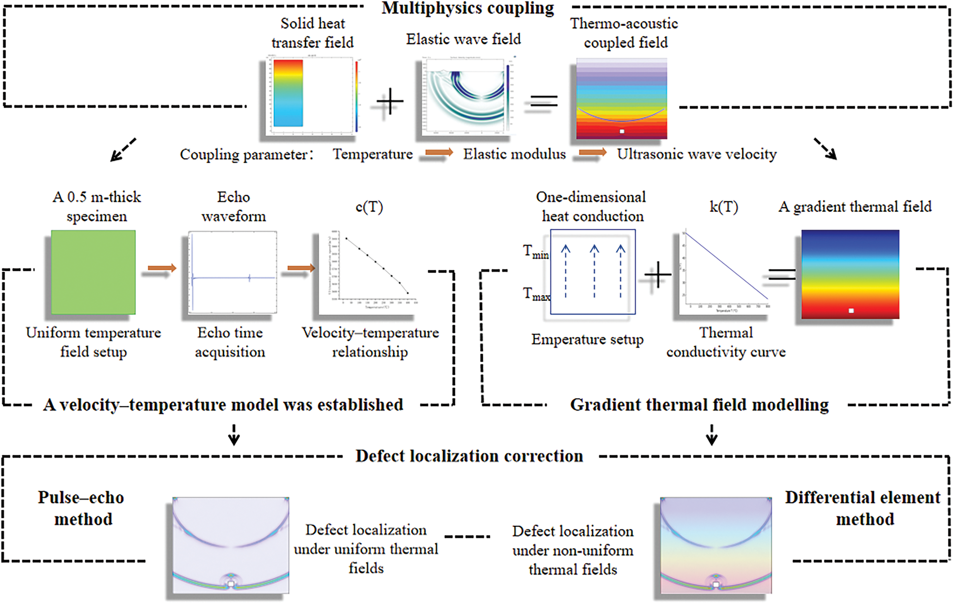
Figure 1: Method framework

2.2 Multiphysics Coupling Modeling Approach

This study focuses on piezoelectric ultrasonic defect localization under the influence of temperature. Coupling the thermal and ultrasonic fields forms the foundation of this work. Here, we present a methodology for coupling the solid heat transfer field with the elastic wave field in the COMSOL platform, providing a reference framework for subsequent investigations.

The constitutive equations (Eqs. (1) and (2)) governing ultrasonic wave propagation in solids indicate that the wave speed, c, depends on the material’s elastic modulus E, Poisson’s ratio ν, and density ρ. Among these parameters, the elastic modulus E is the dominant factor controlling sound velocity. The equations are expressed as follows:

cL=(E(1−ν)ρ(1+ν)(1−2ν))(1)

cs=(Gρ)=(E2ρ(1+ν))(2)

here, c represents the longitudinal wave velocity, E is the elastic (Young’s) modulus, G denotes the shear modulus, ν is Poisson’s ratio, and ρ is the material density. All of these physical parameters are temperature-dependent (T). To investigate the effect of temperature on acoustic velocity, the elastic modulus of 1020 steel was parameterized by expressing E as a function of temperature T and incorporating it into the material properties. The E–T relationship was obtained via polynomial fitting of data extracted from the Manual of Mechanical Engineering Material Property Data, while the other parameters were kept at their default values. The temperature-dependent elastic modulus is given by the following expression (Eq. (3)):

E(T)=−1.18e−07T3+4.667e−05T2−0.06598T+215.2(3)

here, E denotes the elastic modulus and T represents temperature. In this framework, the ultrasonic wave velocity is indirectly affected by the temperature dependence of E. By incorporating this relationship, the thermal field is effectively coupled with the elastic wave physics, enabling the development of a multiphysics model.

2.3 A Modeling Approach to the Sound Velocity-Temperature Relationship

Based on a multiphysics coupling model, a two-dimensional 1020 steel test block with a side length of 0.5 m was subjected to a safe operating temperature range of 20°C–400°C. An excitation source was placed at the center of the upper boundary of the model to simulate piezoelectric ultrasonic [25,26] excitation, as illustrated in Fig. 2. Bottom echo times of the test block were recorded at different temperatures, and the corresponding ultrasonic velocities were calculated using Eq. (4). Because the longitudinal wave produces a more distinct echo, it was chosen as the focus of this study; hereafter, the term “wave velocity” refers to the longitudinal ultrasonic wave velocity. The ultrasonic wave velocity is calculated as follows (Eq. (4)):

c=2Ht(4)

where c is the ultrasonic wave propagation velocity, H is the thickness of the 1020 steel block (0.5 m), and t is the ultrasonic wave propagation time.

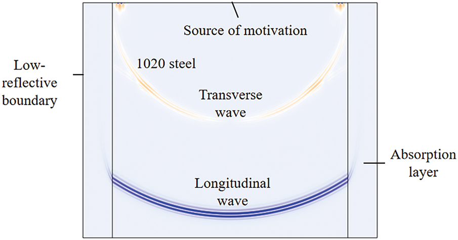
Figure 2: Ultrasonic propagation model

Ultrasonic wave velocities were measured at different temperatures, and a cubic polynomial fit was applied to establish the quantitative relationship between ultrasonic velocity, c, and material temperature, T. This yielded the temperature-dependent ultrasonic velocity model expressed in Eq. (5):

c=a⋅T3+b⋅T2+c⋅T+d(5)

where a, b, c, and d are coefficients, c is the wave velocity, and T is the temperature.

2.4 Modeling Approach for Gradient Temperature Fields

In non-destructive testing, the inspected components are often exposed to non-uniform temperature fields with spatial gradients. Consequently, simulating gradient temperature fields is necessary to provide realistic conditions for subsequent defect localization. Heat transfer in solids is governed by the heat conduction equation, expressed as follows (Eq. (6)):

ρcp∂T∂t=∇⋅(k∇T)+Q(6)

here, ρ is the material density, cp is the specific heat capacity, k is the thermal conductivity, Q denotes the internal heat source, T is temperature, and t represents time. For simplicity, the heat transfer model is reduced to a one-dimensional steady-state thermal conduction problem, while accounting for the temperature dependence of k. The thermal conductivity–temperature relationship was obtained via linear fitting of data from the Manual of Mechanical Engineering Material Property Data, and k was implemented as a temperature-dependent material property. This configuration directly affects the temperature distribution, resulting in a gradient thermal field. The relationship between thermal conductivity and temperature is expressed in Eq. (7):

k(T)=−0.0315T+48.49(7)

where k is the thermal conductivity and T is the temperature. The simplified heat transfer Eq. (8) in the one-dimensional steady-state thermal conduction model is as follows:

ddy(k(T)dTdy)=0(0≤y≤H)(8)

here, H denotes the thickness of the test block (0.5 m), y is the vertical coordinate of the geometric model, and k is the temperature-dependent thermal conductivity. Based on this formulation, heat conduction in a two-dimensional cross-section [27] of the component was simulated, with the ultrasonic propagation direction aligned parallel to the heat transfer direction. Under non-uniform temperature conditions, the temperature-dependent thermal conductivity induces the formation of a gradient thermal field, as illustrated in Fig. 3.

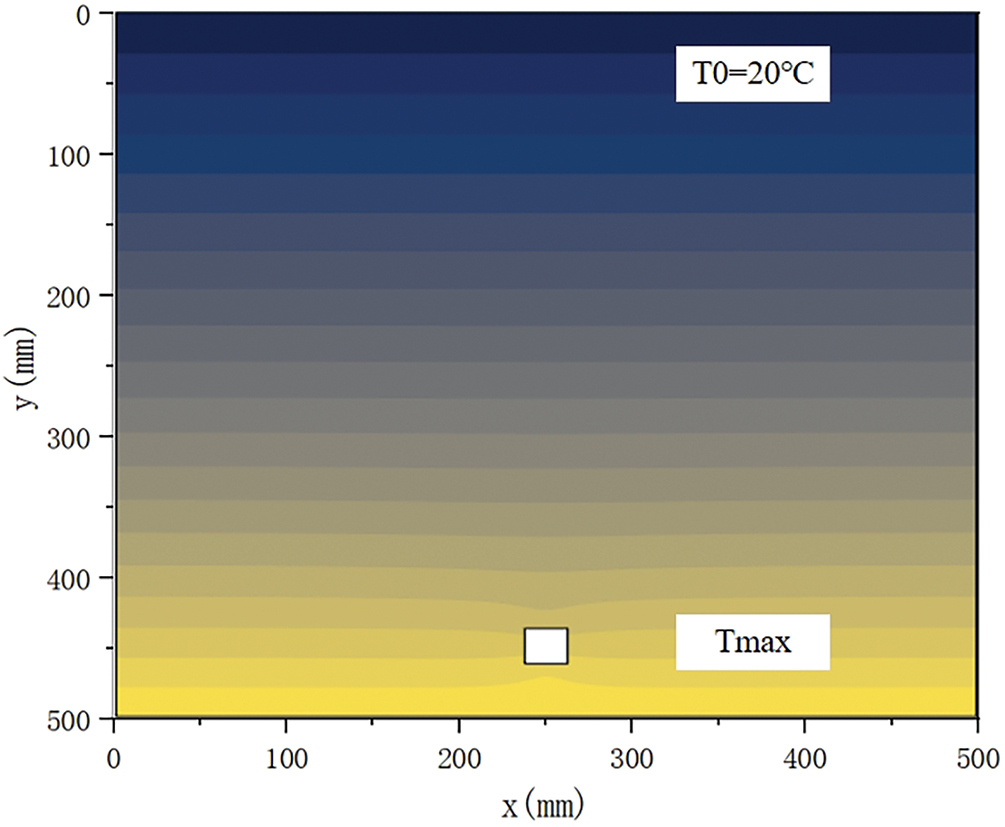
Figure 3: Non-uniform temperature field

2.5 Defect Localization and Correction Method

2.5.1 Defect Localization Correction Method under Uniform Temperature Field

In ultrasonic non-destructive testing, precise defect localization is critical to ensuring detection reliability. To address this, a defect localization model was established by coupling heat transfer in solids with elastic wave propagation, while employing the ultrasonic echo method for quantitative evaluation, as illustrated in Fig. 4. The defect depth is determined from the ultrasonic propagation velocity and the corresponding echo time at which the wave interacts with the defect, as expressed in Eq. (9):

S=c×t2(9)

where S is the calculated position of the defect, c is the propagation velocity of the ultrasonic wave, and t is the echo time at the defect location.

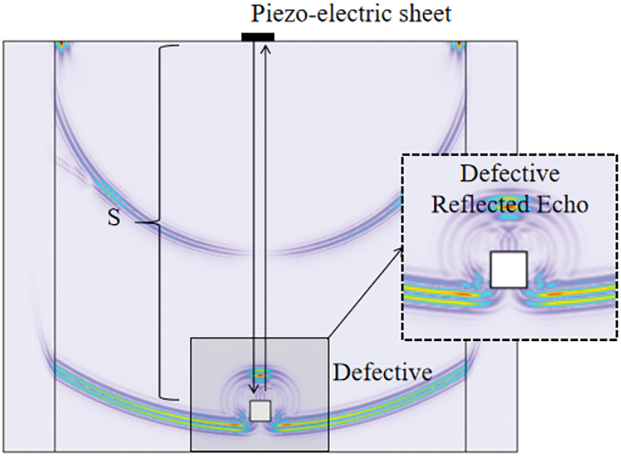
Figure 4: Echo method

Conventional methods typically use the room-temperature sound velocity (20°C) for defect localization. In contrast, the proposed approach accounts for the temperature dependence of ultrasonic wave velocity by introducing the corrected propagation speed. By substituting the velocity–temperature relationship in Eq. (5) together with the measured defect echo time tT1 into Eq. (9), the corrected defect location can be obtained.

2.5.2 Defect Positioning Correction Method in Non-Uniform Temperature Fields

In this study, the thermal conductivity was parameterized as a function of temperature and incorporated into the material properties. This coupling modifies the heat conduction process, thereby shaping the modeled temperature field into a gradient distribution governed by the temperature dependence of k. Using COMSOL numerical simulations, we first obtained the steady-state temperature distribution (Fig. 5). The temperature data along the y-axis were then extracted, and polynomial fitting was applied to derive temperature–position functions for each condition, expressed in Eq. (10):

T(y)=e⋅y2+f⋅y+g(10)

where e, f, g are parameters, T is temperature, and y is the vertical coordinate corresponding to temperature.

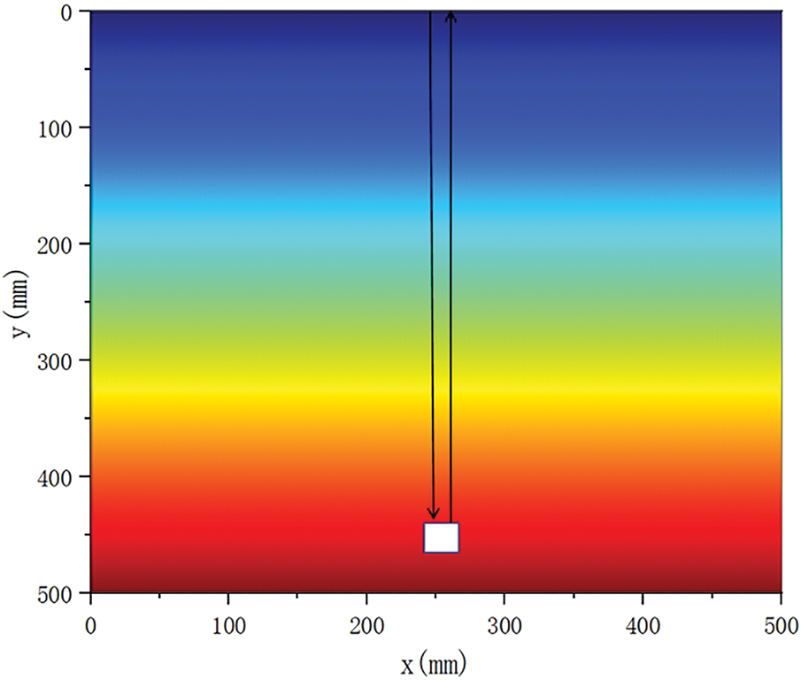
Figure 5: Non-uniform temperature field correction model

Substituting Eq. (10) into the velocity-temperature relation Eq. (5) yields the velocity field function Eq. (11):

c(y)=a⋅[T(y)]3+b⋅[T(y)]2+c⋅T(y)+d(11)

where a, b, c, and d are parameters, c(y) is a function of the sound velocity field, T(y) is a function of the temperature field, and y is the coordinate of the vertical axis of the geometric model.

From Eq. (11), it is evident that the ultrasonic propagation velocity becomes position-dependent within a gradient temperature field, with its value varying continuously along the propagation path. Consequently, the defect position cannot be directly determined using Eq. (5) and the measured echo time t. To address this, we adopt the micro-element method, as illustrated in Fig. 6. In this approach, the total echo time is discretized into 2n segments, each of duration ∆t. The forward propagation from the excitation source [28] to the defect corresponds to n increments of ∆t, with the propagation distance of the n-th segment given by ∆Sn = yn − yn−1.

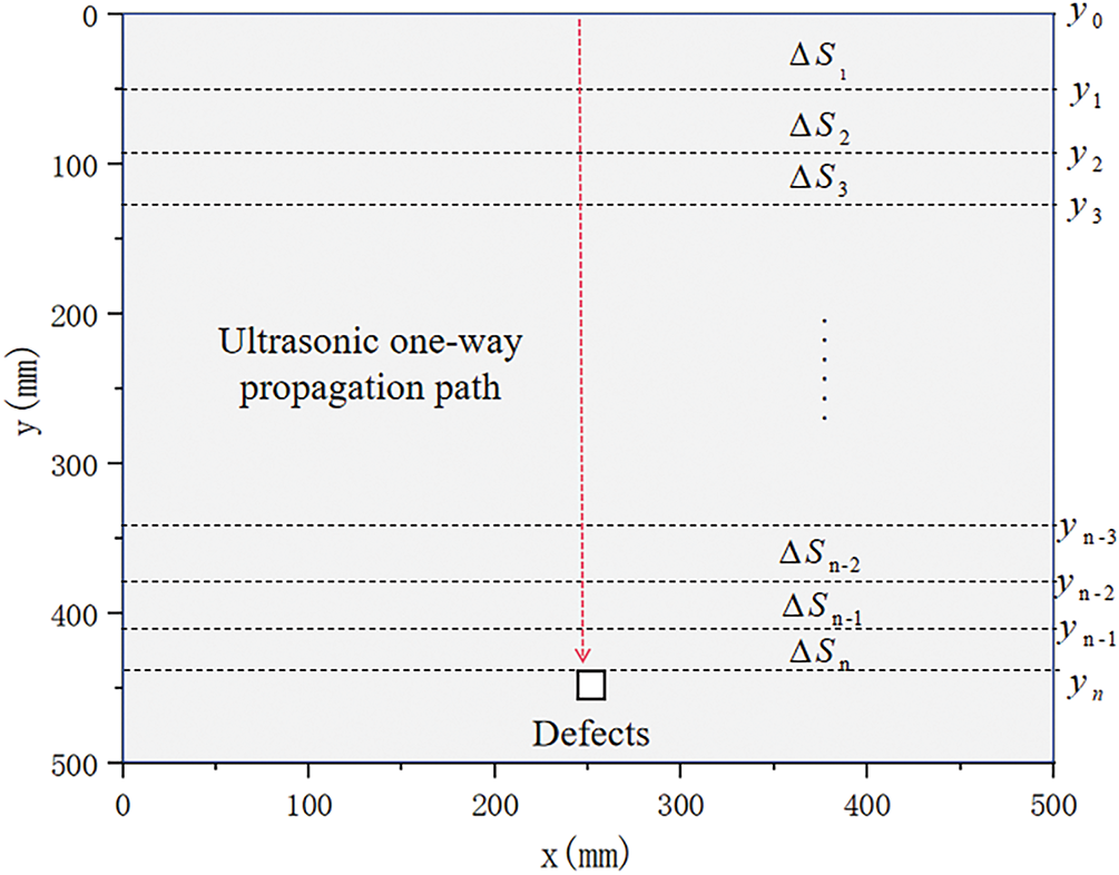
Figure 6: Differential element method

This leads to the correction formula for defect localization Eq. (12):

Sb2=∑i=1nΔSi=yn=yn−1+ΔSn(12)

here, Sb2 denotes the corrected defect location, while ∆Si represents the ultrasonic propagation distance corresponding to the i-th time increment. The coordinates yn and yn−1 refer to successive nodes along the y-axis, and ∆Sn corresponds to the propagation distance within the n-th time segment. When ∆t is sufficiently small, each segment ∆S1, ∆S2, . . . , ∆Sn can be approximated as a locally uniform temperature field. In this case, the ultrasonic wave is assumed to propagate uniformly within ∆Sn at a velocity c(yn−1) defined at node yn−1. Thus, the distance ∆Sn can be obtained from ∆t and c(yn−1), as expressed in Eq. (13):

ΔSn=c(yn−1)×Δt(13)

Substituting Eqs. (13) into (12) gives Eq. (14):

Sb2=yn=yn−1+c(yn−1)×Δt(14)

The initial conditions are further set and Eq. (14) is solved by iterative method as shown in Eq. (15):

{y1=y0+c(y0)×Δty2=y1+c(y1)×Δt…yn−1=yn−2+c(yn−2)×ΔtSb2=yn=yn−1+c(yn−1)×Δt(15)

Combine equations Eqs. (11) and (15), substitute the initial condition y0 = 0 and the corresponding echo time into the combined result, and the corrected defect location under the gradient temperature field can be obtained.

A one-dimensional steady-state heat transfer model was adopted here as a simplified assumption for numerical validation, because such temperature distributions are common in typical components, such as pipes and plates, and because it highlights the fundamental effect of temperature gradients on sound velocity and defect localization errors. Crucially, the proposed microelement integration correction algorithm is independent of the one-dimensional assumption: its only input is the local temperature along the ultrasonic propagation path [29]. Therefore, in practical scenarios with complex boundary conditions or irregular geometries generating two- or three-dimensional temperature fields, the algorithm remains applicable. By obtaining the temperature field via simulation or measurement, extracting temperatures along the ultrasonic path, and mapping them into the temperature-dependent sound velocity relation c = c(T), a corresponding velocity field can be derived. The microelement integration method can then be applied to perform cumulative calculations, enabling accurate defect localization correction under arbitrary temperature distributions.

3  Experimental Analysis

3.1 Sound Velocity-Temperature Relationship Modeling

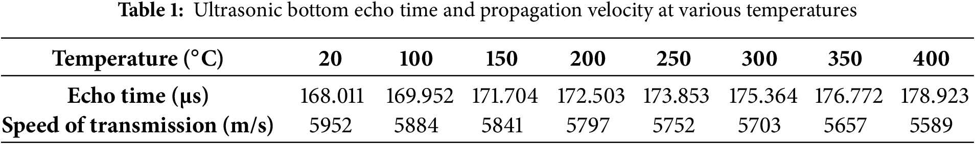
Simulations were conducted on ultrasonic wave propagation under eight uniform temperature fields: room temperature (20°C) and 100°C, 150°C, 200°C, 250°C, 300°C, 350°C, and 400°C. Probes were placed around the signal excitation point to capture pressure-vs.-time curves at each corresponding temperature. To enhance the contrast of bottom echo time data across different temperatures, the results were compiled into a stacked plot, as shown in Fig. 7. After subsequent processing, the bottom echo times were recorded, and the ultrasonic wave velocities in 1020 steel at each temperature were calculated using the ultrasonic velocity Eq. (4). The specific values are listed in Table 1. The data reveals that, with a model thickness of 0.5 m, the ultrasonic wave velocity decreases from 5952 m/s at 20°C to 5589 m/s at 400°C, a reduction of 6.1%. Concurrently, the bottom echo time progressively increases, demonstrating that ultrasonic wave propagation slows as temperature rises.

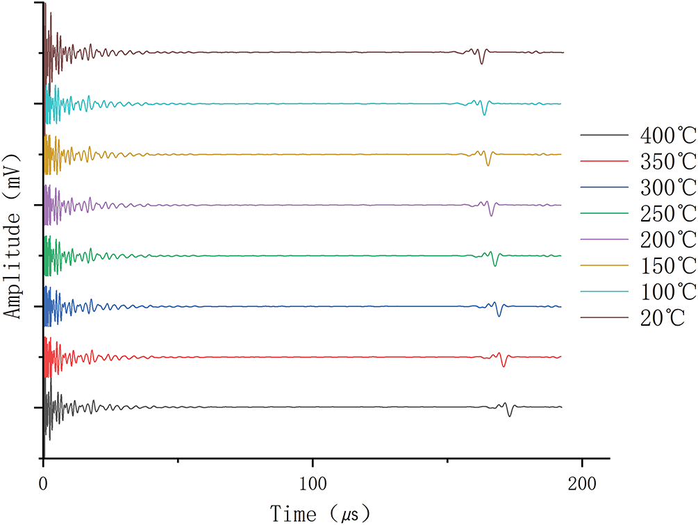
Figure 7: Echo waveform stack diagram

Based on Table 1, regression analysis was performed using the least squares method. The quantitative relationship between ultrasonic propagation velocity c and material temperature T was obtained Eq. (16):

c=−2.142×10−6⋅T3+0.0008702⋅T2−0.9559⋅T+5971(16)

here, c denotes the ultrasonic wave velocity and T the material temperature. The coefficient of determination R2 for the polynomial fitting reaches 0.9996, reflecting excellent agreement between the fitted model and the numerical data. As shown in Fig. 8, the velocity–temperature curve displays a distinctly nonlinear decreasing trend: within the investigated thermal range, ultrasonic velocity decreases progressively with increasing temperature, with the rate of reduction accelerating at higher temperatures. This behavior is fully consistent with classical thermodynamic theory and prior studies on temperature–velocity effects, thereby confirming the robustness of both the experimental procedure and the adopted fitting model.

Figure 8: Speed-temperature curve

3.2 Simulation of Defect Localization Correction under Uniform Temperature Field

A reference defect was embedded at a depth of 0.44 m (y = 0.44 m) from the specimen centerline for simulation analysis (Fig. 4). Uniform temperature fields ranging from 20°C to 400°C were configured, and the corresponding defect echo times were recorded under each condition. The detailed results are summarized in Table 2.

The initial defect location Sa1 was estimated using the room-temperature (20°C) ultrasonic velocity (c0 = 5952 m/s) together with the measured defect echo time tT1, producing the uncorrected localization results listed in Table 3. As temperature increases, the deviation between the calculated and actual defect positions progressively enlarges. This trend highlights the pronounced influence of the temperature–velocity effect on localization accuracy, underscoring the necessity of correction methods for high-temperature ultrasonic testing.

In order to eliminate the temperature effect, this study proposes a correction method based on the sound velocity-temperature relationship by substituting Eqs. (16) into (9) to obtain the following defect location correction Eq. (17):

Sb1=(−2.142×10−6T3+0.0008702T2−0.9559T+5971)tT12(17)

Sb1 represents the corrected defect position, T denotes the model temperature, and tT1 is the echo time at the defect location. By substituting the temperature T and corresponding echo time tT1 from Table 2 into equation Eq. (17), the corrected defect positioning values under different temperatures in a uniform temperature field are obtained, as listed in Table 4.

Under a uniform temperature field, the calculated defect locations with and without correction are compared in Fig. 9. Without correction, the apparent defect depth increases systematically with temperature, leading to a progressive divergence from the true location, with deviations reaching up to 6.5% at 400°C. By contrast, the corrected results remain essentially coincident with the actual defect positions across the full temperature range, with the maximum deviation limited to 0.05%. This demonstrates that the correction strategy effectively eliminates temperature-induced bias in ultrasonic measurements, thereby providing a robust pathway for reliable defect quantification in high-temperature environments.

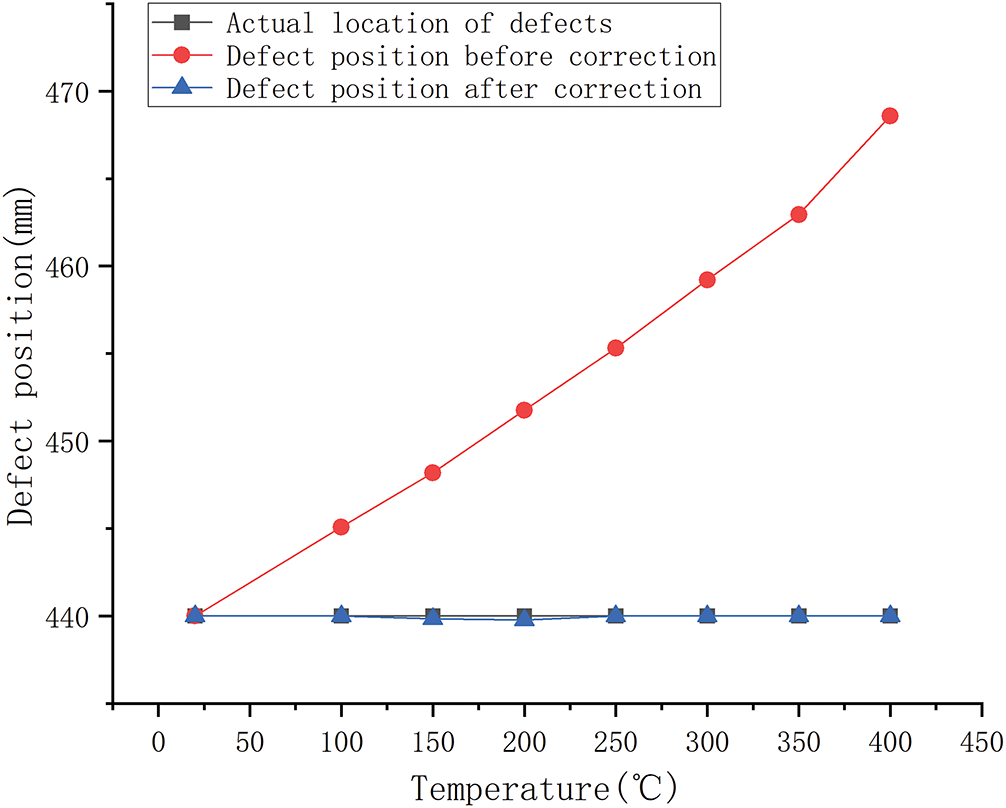
Figure 9: Uniform temperature field defect location

3.3 Simulation of Defect Localization Correction under Non-Uniform Temperature Field

As described in Section 2.5.2, the correction method for defect localization under a non-uniform temperature field was implemented by constructing a one-dimensional heat transfer model in COMSOL. The upper boundary was fixed at 20°C to simulate convective cooling, while the lower boundary was set to the maximum temperature Tmax. Seven high-temperature conditions ranging from 100°C to 400°C (increments of 50°C) were applied (Fig. 3). The temperature distribution was obtained by embedding the temperature-dependent thermal conductivity k(T) into the material properties and solving numerically. Temperature data along the y-axis were extracted and fitted with polynomial functions to yield the temperature–position relationships for each case (Table 5). The corresponding profiles are plotted in Fig. 10, showing that temperature increases monotonically with depth, with the slope of the curve steepening in deeper, hotter regions. This indicates that the temperature gradient is larger at high temperatures and smaller at low temperatures, consistent with the physical principle that the thermal conductivity of 1020 steel decreases with temperature. Reduced conductivity at elevated temperatures suppresses heat transport, thereby producing steeper local gradients.

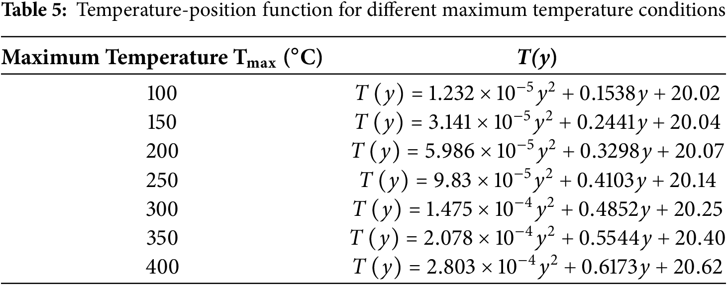
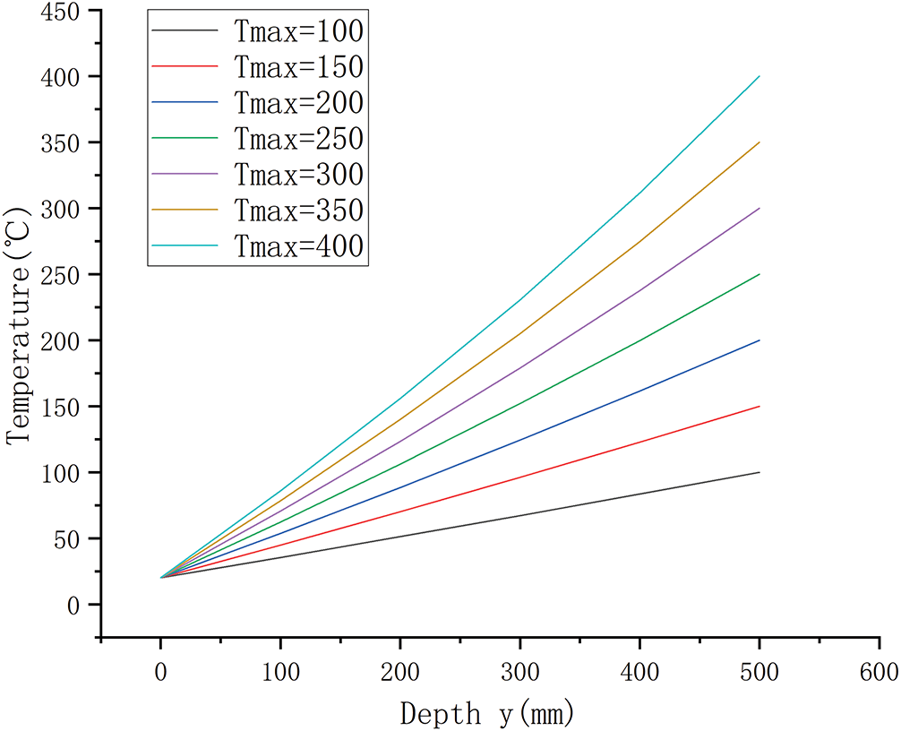
Figure 10: Temperature—depth curve

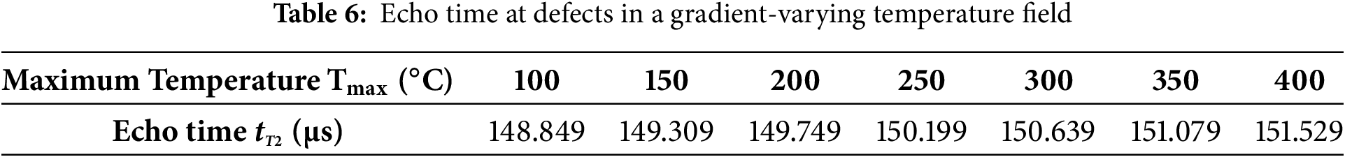
As shown in Fig. 3, a two-dimensional model of 1020 steel with an edge length of 0.5 m and a defect location at y = 0.44 m was used as the study object, and the ultrasonic echo time at the defect location was collected under seven sets of temperature fields, as shown in Table 6.

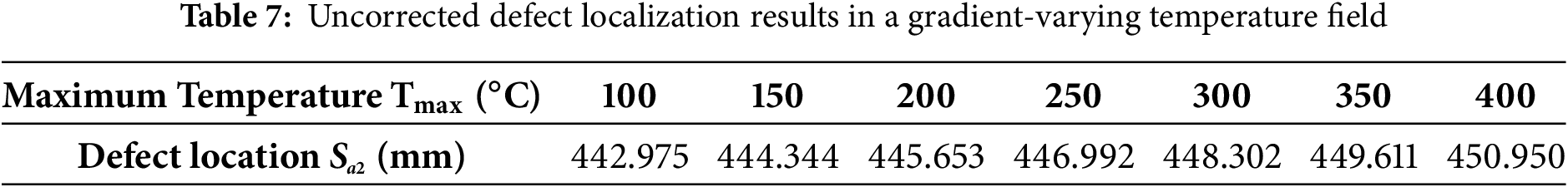
Defect localization was first evaluated using the conventional ultrasonic echo method [30,31]. The room-temperature sound velocity (c = 5952 m/s at 20°C) and the echo times tT2 from Table 6 were substituted into Eq. (9) to calculate uncorrected defect positions under seven gradient-varying temperature fields (Table 7). The results show a trend consistent with the single-temperature case (Table 3): deviations in defect position increase with rising temperature. Notably, however, the errors in gradient-varying fields are substantially smaller. This reduction can be attributed to the lower average temperature of the gradient-varying fields, which yields a higher effective sound velocity that more closely reflects room-temperature propagation conditions.

Substituting the temperature field functional T(y) from Table 5 into the sound velocity-temperature relation Eq. (16) yields the sound velocity field functional as shown in Eq. (18):

c(y)=−2.142×10−6[T(y)]3+0.0008702[T(y)]2−0.9559T(y)+5971(18)

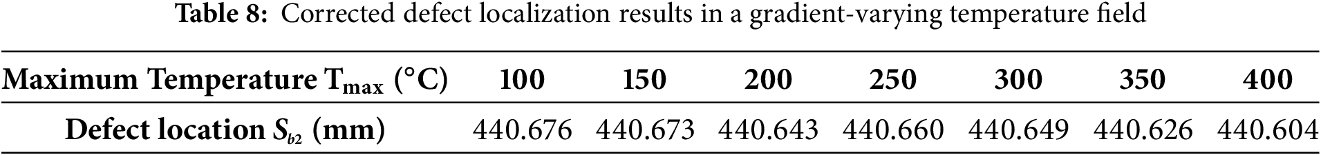
Next, the microelement method is utilized to calculate the defect location, as shown in Fig. 6, and associating Eqs. (11) and (15), and substituting the corresponding temperatures and echo times in the gradient-varying temperature field to obtain the corrected defect location under the gradient-varying temperature field, as shown in Table 8.

The defect localization results obtained under gradient-varying temperature fields, both uncorrected (Table 7) and corrected (Table 8), are compared in Fig. 11. The uncorrected results show a clear temperature dependence: localization deviations increase progressively with temperature, reaching a maximum of 2.5% at 400°C. In contrast, the corrected results nearly coincide with the true defect position across the entire temperature range, with deviations not exceeding 0.15%. This demonstrates that the correction method markedly enhances localization accuracy compared with conventional calculations.

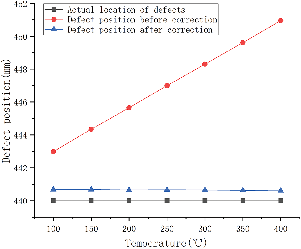
Figure 11: Defect location in non-uniform temperature fields

It should be noted that, for numerical validation, a two-dimensional test block with a side length of 0.5 m was used for systematic parameter analysis and algorithm verification. The primary purpose of this model was to confirm the methodology and assess numerical stability; it serves solely for validation. The results indicate that when the temperature gradient within the component is small, the proposed correction method has limited impact, whereas its effectiveness becomes pronounced under larger temperature gradients. In industrial applications, component sizes typically range from millimeters to meters. Smaller components generally exhibit minor internal temperature gradients, while larger components are prone to substantial gradients, amplifying the spatial modulation of sound velocity. Consequently, the temperature-field-based microelement integration correction method presented here is particularly suited for large-scale components in practical engineering scenarios.

4  Conclusions

This study proposes a defect localization correction method that integrates multi-physics coupled modeling with dynamic sound velocity tracking to address localization errors caused by non-uniform temperature fields in high-temperature ultrasonic inspection. By incorporating temperature-dependent material properties into a two-dimensional thermoacoustic model and discretizing the ultrasonic propagation process through a microelement integration approach, the method effectively reconstructs the sound velocity distribution and reduces localization deviations induced by thermal gradients. Compared with conventional uniform-temperature correction models, it demonstrates a significant improvement in accuracy, providing a high-precision tool for online ultrasonic inspection of industrial systems such as nuclear power pipelines and aero-engines. These findings lay the foundation for enhancing the accuracy and reliability of ultrasonic non-destructive testing under elevated temperatures.

The central focus of this method lies in correcting the influence of internal temperature fields within the inspected structure on sound velocity and defect localization. It should also be noted, however, that temperature not only affects ultrasonic propagation inside the specimen but also impacts the transducer and its measurement system (for instance, the sensitivity of piezoelectric materials decreases near their Curie temperature). Future work will integrate the proposed correction algorithm with established transducer temperature-adaptive strategies—such as waveguides or high-temperature wedges, active cooling designs, high-Curie-point piezoelectric materials, and, under extreme conditions, non-contact ultrasonic technologies—to further enhance the robustness and applicability of ultrasonic evaluation in harsh thermal environments.

Acknowledgement: This study was funded by the Non-Destructive Testing Research Group of the School of Mechanical Engineering, Inner Mongolia University of Science and Technology, and supported by the Inner Mongolia Special Equipment Inspection and Research Institute.

Funding Statement: This study was supported by the following projects: National Natural Science Foundation of China [U24A20135]; Science and Technology Program of the State Administration for Market Regulation [2024MK016]; Basic Scientific Research Fund Project for Higher Education Institutions of Inner Mongolia (2024YXXS057); Key Project of Natural Science Foundation of Inner Mongolia [2023ZD12]; 2023 Inner Mongolia Autonomous Region Key R&D and Achievement Transformation Program [2023YFHH0090]; Natural Science Foundation of Inner Mongolia [2022MS05006]; Talent Development Fund of Inner Mongolia Autonomous Region; Fundamental Research Funds for Universities [2023RCTD012]; Fundamental Research Funds for Universities [2023QNJS075]; Inner Mongolia Autonomous Region Postgraduate Research Innovation Project [KC2024053B]; Fundamental Research Funds for Universities [2024YXXS012]; Open Project of the National Key Laboratory of Special Vehicle Design and Manufacturing Integration Technology [GZ2023KF012].

Author Contributions: The authors confirm contribution to the paper as follows: Conceptualization, Jianhua Du and Shaofeng Wang; methodology, Jianhua Du; software, Ting Gao; validation, Jianhua Du, Huiwen Sun and Wenjing Liu; formal analysis, Shaofeng Wang; investigation, Ting Gao; resources, Huiwen Sun; data curation, Wenjing Liu; writing—original draft preparation, Jianhua Du; writing—review and editing, Shaofeng Wang; visualization, Wenjing Liu; supervision, Jianhua Du; project administration, Ting Gao; funding acquisition, Wenjing Liu. All authors reviewed the results and approved the final version of the manuscript.

Availability of Data and Materials: The data is included in the article.

Ethics Approval: Not applicable.

Conflicts of Interest: The authors declare no conflicts of interest to report regarding the present study.

References

1. Quaegebeur N, Masson P, Berry A, Ardin C, D’Anglade PM. Ultrasonic non-destructive testing of cardboard tubes using air-coupled transducers. NDT E Int. 2018;93:18–23. doi:10.1016/j.ndteint.2017.09.011. [Google Scholar] [CrossRef]

2. Hassani S, Dackermann U. A systematic review of advanced sensor technologies for non-destructive testing and structural health monitoring. Sensors. 2023;23(4):2204. doi:10.3390/s23042204. [Google Scholar] [PubMed] [CrossRef]

3. Kurashkin KV, Gonchar AV, Klyushnikov VA, Mishakin VV. Effect of microstructure on temperature dependence of ultrasonic velocity in aluminum. Acoust Phys. 2023;69(3):335–40. doi:10.1134/s1063771022600589. [Google Scholar] [CrossRef]

4. Chang RR, Shu CM, Chang MK, Chow NM. Prediction of error caused by temperature effects in ultrasonic thickness measurement. Mater Eval. 2004;62(1):69–72. [Google Scholar]

5. Wu Y, Han L, Gong H, Ahmad AS. A modified model for simulating the effect of temperature on ultrasonic attenuation in 7050 aluminum alloy. AIP Adv. 2018;8(8):085003. doi:10.1063/1.5045627. [Google Scholar] [CrossRef]

6. Van De Wyer N, Schram C, Van Dyck D, Dierckx M. The effect of non-uniform temperature and velocity fields on long range ultrasonic measurement systems in MYRRHA. IEEE Trans Nucl Sci. 2016;64(2):829–36. doi:10.1109/TNS.2016.2642342. [Google Scholar] [CrossRef]

7. Zhang Y, Ming T, Li J. Study on the influence of temperature on ultrasonic pressure measurement technology. J Phys Conf Ser. 2022;2174(1):12008. doi:10.1088/1742-6596/2174/1/012008. [Google Scholar] [CrossRef]

8. Stevenson T, Wang C. Velocity compensation and practical aspects for high-temperature ultrasonic testing. Insight-Non-Destr Test Cond Monit. 2021;63(11):641–7. doi:10.1784/insi.2021.63.11.641. [Google Scholar] [CrossRef]

9. Liu W, Hu J, Lv F, Tang Z. A new method for long-term temperature compensation of structural health monitoring by ultrasonic guided wave. Measurement. 2025;252:117310. doi:10.1016/j.measurement.2025.117310. [Google Scholar] [CrossRef]

10. Wei D, Yang X, Shi Y, Xiao G, Du Y, Gui Y. A method for reconstructing two-dimensional surface and internal temperature distributions in structures by ultrasonic measurements. Renew Energy. 2020;150:1108–17. doi:10.1016/j.renene.2019.10.081. [Google Scholar] [CrossRef]

11. Aslam M, Nagarajan P, Remanan M. Defect localization using nonlinear lamb wave mixing technique. J Nondestruct Eval. 2021;40(1):16. doi:10.1007/s10921-020-00747-5. [Google Scholar] [CrossRef]

12. Ho CY, Powell RW, Liley PE. Thermal conductivity of the elements. J Phys Chem Ref Data. 1972;1(2):279–421. doi:10.1063/1.3253100. [Google Scholar] [CrossRef]

13. Li W, Kou H, Zhang X, Ma J, Li Y, Geng P, et al. Temperature-dependent elastic modulus model for metallic bulk materials. Mech Mater. 2019;139:103194. doi:10.1016/j.mechmat.2019.103194. [Google Scholar] [CrossRef]

14. Li Q, Luo Z, Zhou S. Novel baseline-free ultrasonic Lamb wave defect location method based on path amplitude matching. Meas Sci Technol. 2024;35(6):65111. doi:10.1088/1361-6501/ad329a. [Google Scholar] [CrossRef]

15. Liu Y, Zhou X, Zhu J, Yu J, Dong C, He Z, et al. Sound waves tracing method in temperature-velocity coupling field of nuclear reactor. Appl Therm Eng. 2025;258:124658. doi:10.1016/j.applthermaleng.2024.124658. [Google Scholar] [CrossRef]

16. Yang Y, Dai K, Yin Q, Li C, Li H, Zhang H. Multiphysics coupling simulation of electromagnetic railgun based on the field-circuit coupled method. J Magn Magn Mater. 2024;607:172403. doi:10.1016/j.jmmm.2024.172403. [Google Scholar] [CrossRef]

17. Ramezani H, Jamali-Rad H, Leus G. Target localization and tracking for an isogradient sound speed profile. IEEE Trans Signal Process. 2013;61(6):1434–46. doi:10.1109/TSP.2012.2235432. [Google Scholar] [CrossRef]

18. Biagiotti SF. Effect of temperature on ultrasonic velocity in steel. In: Proceedings of the Corrosion 1997; 1997 Mar 9–14; New Orleans, LA, USA. p. 1–9. doi:10.5006/c1997-97259. [Google Scholar] [CrossRef]

19. Li L, Zheng H. Numerical simulation of ultrasonic heat meter by multiphysics coupling finite-element simulation software. Therm Sci. 2020;24(5B):3309–217. doi:10.2298/tsci191106122l. [Google Scholar] [CrossRef]

20. Cegla FB, Jarvis AJC, Davies JO. High temperature ultrasonic crack monitoring using SH waves. NDT E Int. 2011;44(8):669–79. doi:10.1016/j.ndteint.2011.07.003. [Google Scholar] [CrossRef]

21. Atkinson I, Gregory C, Kelly SP, Kirk KJ. Ultrasmart: developments in ultrasonic flaw detection and monitoring for high temperature plant applications. In: Proceedings of the ASME 2007 Pressure Vessels and Piping Conferencel; 2007 Jul 22–26; San Antonio, TX, USA. p. 573–85. doi:10.1115/CREEP2007-26411. [Google Scholar] [CrossRef]

22. Vajdi M, Moghanlou FS, Sharifianjazi F, Asl MS, Shokouhimehr M. A review on the comsol multiphysics studies of heat transfer in advanced ceramics. J Compos Compd. 2019;2(1):35–44. doi:10.29252/jcc.2.1.5. [Google Scholar] [CrossRef]

23. Bazargan M, Almqvist BSG, Motra HB, Broumand P, Schmiedel T, Hieronymus CF. Elastic wave propagation in a stainless-steel standard and verification of a COMSOL multiphysics numerical elastic wave toolbox. Resources. 2022;11(5):49. doi:10.3390/resources11050049. [Google Scholar] [CrossRef]

24. Ghose B, Balasubramaniam K, Krishnamurthy CV, Rao AS. COMSOL based 2D FEM model for ultrasonic guided wave propagation in symmetrically delaminated unidirectional multilayered composite structures. In: Proceedings of the National Seminar and Exhibition on Nondestructive Evaluation; 2011 Dec 8–10; Chennai, India. p. 45–9. [Google Scholar]

25. Cai J, Zhang H, Miao H. Excitation of unidirectional SH wave within a frequency range of 50 kHz by piezoelectric transducers without frequency-dependent time delay. Ultrasonics. 2022;118:106579. doi:10.1016/j.ultras.2021.106579. [Google Scholar] [PubMed] [CrossRef]

26. Du P, Chen W, Deng J, Zhang S, Zhang J, Liu Y. A critical review of piezoelectric ultrasonic transducers for ultrasonic-assisted precision machining. Ultrasonics. 2023;135:107145. doi:10.1016/j.ultras.2023.107145. [Google Scholar] [PubMed] [CrossRef]

27. Abimbola A, Bright S. Alternating-direction implicit finite-difference method for transient 2D heat transfer in a metal bar using finite difference method. Int J Sci Eng Res. 2015;6(6):105–8. doi:10.14299/ijser.2015.06.013. [Google Scholar] [CrossRef]

28. Lap-Arparat P, Tuchinda K. Development of temperature-strain prediction based on deformation-induced heating mechanism in SCM440 surface cracked shaft under ultrasonic excitation. Int J Eng. 2024;37(1):151–66. doi:10.5829/ije.2024.37.01a.14. [Google Scholar] [CrossRef]

29. Wu Y, Zhang W, Zhang T, Wu Y, Yang X. Study on ultrasonic propagation path in nonuniform temperature field. Russ J Nondestruct Test. 2021;57(11):968–75. doi:10.1134/s1061830921110115. [Google Scholar] [CrossRef]

30. Ivanchev I. Experimental determination of dynamic modulus of elasticity of concrete with ultrasonic pulse velocity method and ultrasonic pulse echo method. IOP Conf Ser Mater Sci Eng. 2022;1252(1):012018. doi:10.1088/1757-899x/1252/1/012018. [Google Scholar] [CrossRef]

31. Zheng S, Zhang S, Luo Y, Xu B, Hao W. Nondestructive analysis of debonding in composite/rubber/rubber structure using ultrasonic pulse-echo method. Nondestruct Test Eval. 2021;36(5):515–27. doi:10.1080/10589759.2020.1825707. [Google Scholar] [CrossRef]