Block-Wise Sliding Recursive Wavelet Transform and Its Application in Real-Time Vehicle-Induced Signal Separation

1  Introduction

In the daily use of bridges, the structures are exposed to various vertical loads, which can be generally divided into two categories: dynamic loads caused by the passage of vehicles and static loads induced by environmental factors. Individual vehicle loads produce spatially localized dynamic responses, resulting in a temporal “peaking” effect in the monitoring signal. The static load, mainly caused by environmental factors such as temperature, is reflected as a long-term overall variation in the monitoring signal. In the application of structural health monitoring (SHM) systems, the evaluation and diagnosis of bridge damage often require only the static load response (static signal), while vehicle weight identification uses only the vehicle-induced dynamic signal. However, during sensor sampling, these two types of signals are coupled, making the development of signal separation algorithms necessary. In recent years, with the development of structural monitoring technology, data analysis in many studies is no longer confined to a fixed segment of data but to a real-time data stream [1–3]. Therefore, the development of algorithms for the real-time separation of vehicle-induced and static signals has become a more important and urgent issue.

Approaches to separating vehicle-induced dynamics and static trends in SHM fall broadly into temperature-assisted and signal-only categories. In the temperature-assisted category, the static response is inferred from the correlation between temperature and strain—via, for example, Square-Root Slope Function (SRSF), Bayesian warping, nighttime correlation analysis, deep kernel regression, iterative regression, or spatiotemporal Dynamic Convolution Neural Network-Long Short-Term Memory (DCNN-LSTM) modeling—thereby achieving separation through prediction [4–8]. In the signal-only category, the total response is decomposed using time–frequency analysis or learning-based methods, including wavelet analysis, Empirical Mode Decomposition (EMD), LSTM-based extraction, Variational Mode Decomposition (VMD)/EMD for online separation [9–12], and online Kalman filtering [13,14].

Despite their utility, both families face limitations in achieving real-time separation of vehicle-induced responses. The temperature–strain correlation often exhibits temporal lag and site-dependent variability that are difficult to quantify, reducing prediction accuracy [15–18]. Within signal-only methods, linear filters are computationally efficient but often lack separation precision, whereas nonlinear iterative techniques (e.g., EMD, VMD) and online Kalman filtering incur high computational and memory costs and show strong dependence on model assumptions and parameter tuning, which limits their efficiency for high-frequency data streams [9–12]. These limitations highlight the need for a deterministic, model-free approach capable of processing streaming data with bounded latency and predictable computational demand [13,14].

The Discrete Wavelet Transform (DWT) provides lower computational complexity than Continuous Wavelet Transform (CWT) or VMD and is supported by a well-established theoretical foundation [19]. In the field of structural health monitoring, the application of DWT can be roughly divided into two categories [20]. The first category involves decomposing the original signal to extract time–frequency features, mainly for signal anomaly detection [21,22] and structural condition assessment [23,24]. The second category involves decomposition and reconstruction of the original signal to extract specific components, with applications including denoising of seismic waves [25], pavement sensor signal processing [26], extraction of transient structural responses [27], fatigue history editing [28], and vehicle-induced response extraction in bridges [29]. However, in all these studies, wavelet decomposition and reconstruction were performed on fixed-length datasets, rather than on real-time streaming signals.

Therefore, it is essential to develop a wavelet transform algorithm capable of operating efficiently in real-time streaming environments. Such an algorithm can not only improve the efficiency of vehicle-induced signal separation for real-time monitoring but also benefit other engineering fields requiring online signal processing. This paper proposes a Block-wise Sliding Wavelet Transform (BSWT) and its recursive variant (BSRWT) for streaming signal separation. We first outline the BSWT framework for streaming deployment, then present the recursive boundary-aware update scheme (BSRWT), and finally evaluate both approaches on simulated and field data. Compared with recursive EMD/VMD (which are iterative, parameter-sensitive, and computationally intensive) and online Kalman filtering (which is model-dependent and tuning-intensive for nonstationary multi-component mixtures), the proposed framework is deterministic, model-free, and resource-bounded, featuring an explicit latency control and a closed-form complexity behavior.

This work contributes three main innovations for streaming SHM. First, wavelet-based separation is reformulated into a block-wise sliding pipeline that produces continuous outputs under a fixed, user-controllable delay. Second, a recursive reuse mechanism is introduced across adjacent windows, so that the per-update cost scales with the decomposition depth and filter length rather than with the full window size, enabling strict real-time operation without iterative optimization. Third, a latency–accuracy analysis is presented, offering a practical delay selection strategy that mitigates sliding-window boundary distortions while maintaining bounded latency.

2  Block-Wise Sliding Wavelet Transform

2.1 Signal Extraction and Decomposition

2.1.1 Signal Separation within a Single Time Window

Vehicle-induced signal separation within a single time window requires first obtaining the static signal from the original signal using the Discrete Wavelet Transform (DWT), which consists of two main steps: decomposition and reconstruction. In the decomposition step, the original signal is divided into multiple layers, and at each layer, the signal is separated into a detail component and an approximation component. In the reconstruction step, only the approximation component from the highest layer is used to reconstruct the signal, while all detail components are discarded. The reconstructed signal represents the static component of the original signal. The vehicle-induced signal is then obtained by subtracting the static component from the original signal.

The flowchart of the algorithm is shown in Fig. 1 (an example of a three-layer DWT). “A” followed by a number denotes the approximation component at the corresponding layer, “D” denotes the detail component, and “R” denotes the reconstructed signal. Two parameters must be determined in this algorithm: the number of decomposition layers and the wavelet basis function. The wavelet basis function defines the coefficients of the high-pass and low-pass filters, as well as the reconstruction filters used in the process.

Figure 1: Flowchart of DWT

The process of decomposition and reconstruction mainly refers to the Mallet fast algorithm [30,31], which will be briefly reviewed in Sections 2.1.1 and 2.1.2. Some details in the convolution on the data boundary will also be elaborated.

2.1.2 Decomposition

In the decomposition step, the original signal (also denoted as the approximate signal of layer 0th) is firstly convolved with the high-pass filter, and the signal obtained after convolution is downsampled by half of its length to get the detailed signal of the 1st layer. The original signal is also convolved with the low-pass filter and downsampled by half of its length to get the approximate signal of the 1st layer. Then, the approximate signal of the 1st layer is convolved with the high-pass filter and the low-pass filter respectively and then downsampled to get the detail and approximate signal of the 2nd layer.

Let n be the number of decomposition layers. The process is shown in the following equation:

Aj+1(i)=∑k=1lL(k)Aj(2i−k)(1)

Dj+1(i)=∑k=1lH(k)Aj(2i−k)(2)

where 0≤j<n and j denotes the number of layers of the signal. i in the brackets represents the sequence number in the signal. The length of the signal of Aj+1 is half of that of Aj. l represents the length of the filter. L and H stand for the low-pass filter and high-pass filter, respectively.

It should be noted that the length of the series should remain the same after the convolution is done. Therefore, it is inevitable that a number of zeros need to be added to the beginning or end of the series during the convolution. Fig. 2 below shows the process of convolution when adding a number of zeros at the beginning of the previous signal during the process of calculating Aj+1 from Aj.

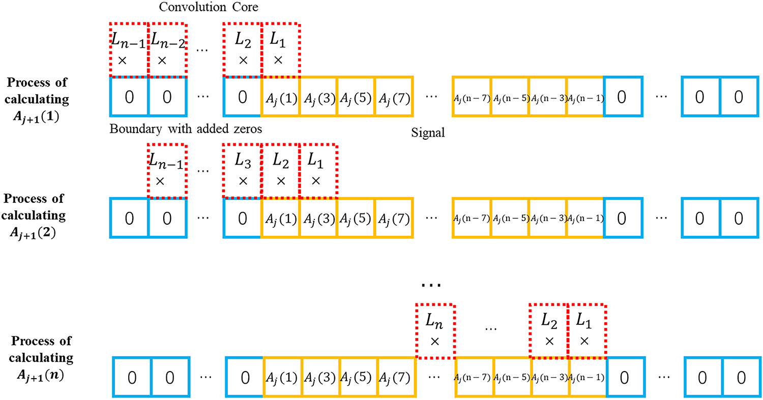
Figure 2: The convolution on the signal boundary in decomposition

In the process of wavelet decomposition, each layer of the detail signal contains the high-frequency information of the approximation signal from the previous layer. As the decomposition progresses, more high-frequency information is gradually removed, leaving only the lower-frequency content that represents the overall trend of the signal. When the original data undergoes multi-layer decomposition, the resulting approximation signal becomes progressively shorter in length. After several layers of decomposition, the final approximation signal obtained serves as the input for the reconstruction process.

2.1.3 Reconstruction

In this section, we describe how to reconstruct the approximate signal at the nth layer into a signal of the same length as the original input. Although wavelet reconstruction can incorporate multiple layers of detail and approximation information, in this study it is sufficient to use only the highest-level approximation signal, since the objective is to extract the static component of the signal.

During reconstruction, the approximate signal from the nth layer is first upsampled by inserting zeros between adjacent data points. For example, if the approximate signal from the previous layer is {1, 2, 3, 4, 5, 6}, the upsampled signal becomes {0, 1, 0, 2, 0, 3, 0, 4, 0, 5, 0, 6}. After upsampling, the sequence is convolved with the reconstruction filter to obtain the reconstructed signal for the previous layer. Unlike the decomposition process, zeros are appended to the end of the signal during convolution to ensure that the reconstructed signal maintains the same length as the input signal. This procedure forms the basis of the wavelet reconstruction process described in this study.

Rj~(i)={Rj+1(i2+1),nis even number0,nis odd number(3)

Rj(i)=∑k=1lF(k)Rj~(i−k)(4)

where F represents the reconstruction filter, j represents the number of the layer of reconstructed signal, 0≤j<n. The nth layer’s reconstructed signal is the An obtained in the decomposition process and the 0th layer is the static signal separated from the original signal. Therefore, the vehicle-induced signal can be obtained by subtracting the static signal from the original signal.

2.2 Real-Time Signal Stream Separation by Window Sliding

In the previous section, the process of separating vehicle-induced signals using the wavelet transform within a fixed time window was introduced. However, in real-time monitoring, the input to the algorithm is a continuously updating data stream rather than a fixed-length signal segment. To address this, a sliding-window approach is adopted, as illustrated in Fig. 3.

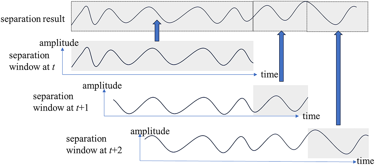
Figure 3: Sliding-window process of a real-time signal separation system

First, an initial window is defined, within which the wavelet transform is applied to perform signal separation. This window must be sufficiently large to ensure that the vehicle-induced response can be clearly distinguished from the static response. Afterward, whenever a new data point is received from the sensor, the extraction window shifts forward, and the same wavelet transform algorithm with identical parameters is applied to the updated window for signal separation. The end portion of the new separation result is then appended to the previous results. As the window continues to slide, the signal is separated in real time.

Through this mechanism, the Block-wise Sliding Wavelet Transform (BSWT) achieves real-time signal separation. However, two significant limitations remain. First, for adjacent windows, most computations are repeated, resulting in low computational efficiency. Second, because the final separated signal is formed by concatenating results at the window boundaries, it is subject to a strong boundary effect, which may reduce separation accuracy. To address these issues, the Block-wise Sliding Recursive Wavelet Transform (BSRWT) is proposed. This method utilizes data from adjacent windows to improve the efficiency of BSWT and introduces a controlled delay to enhance accuracy. Specifically, the recursive scheme reuses information from the previous window, allowing each update to process only the newly entered and soon-to-exit data points at each decomposition level. Consequently, the computational cost per update depends only on the number of decomposition levels and the filter length, rather than on the total window size.

3  Block-Wise Sliding Recursive Wavelet Transform

3.1 Recursive Wavelet Transform

As shown in Fig. 4, during the window-sliding process for data separation, the signal in each subsequent window is shifted forward by one sample relative to the previous window, and it terminates with a new data point received from the sensor. The recursive wavelet transform leverages this property in real-time signal transmission to reduce algorithmic complexity and enhance computational efficiency.

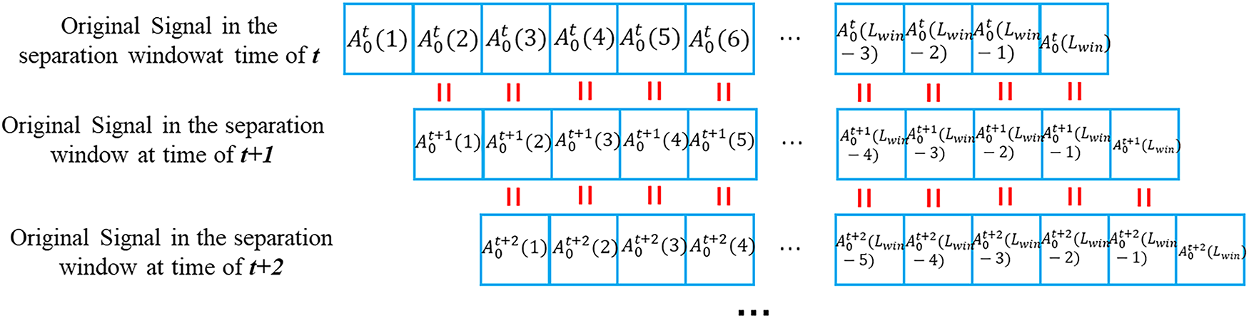
Figure 4: The feature of signal in adjacent sliding windows

In this section, superscripts of the letter symbols denote the time dimension, subscripts indicate the decomposition level in the wavelet transform, and numbers in brackets represent the index position within the data sequence.

3.1.1 Recursive Decomposition

The equivalent decomposition process is performed with reference to the stationary wavelet transform (SWT) method [32,33]. Unlike the commonly used discrete wavelet transform (DWT), the SWT does not downsample the data at each level when computing the next layer of wavelet coefficients; instead, it upsamples the convolution kernel at each stage.

Assume that the wavelet decomposition has n levels. The convolution kernel at the kth level is denoted as Gk, while G0 represents the convolution kernel applied directly to the original signal. G0 corresponds to the low-pass filter coefficients, which are determined solely by the selected wavelet basis function.

In the standard DWT, when calculating the approximation signal at the second level, the first-level convolved signal must be further convolved with the low-pass filter after downsampling. This process is equivalent to performing the convolution without downsampling, but using a modified convolution kernel in which zeros are inserted at regular intervals, followed by downsampling after the convolution is completed.

Therefore, the process of downsampling and convolution in DWT can be replaced by the following process: the original signal is convolved with G0, G1…Gn−1 to obtain the series A1, A2…An and after that An is downsampled (take 1 every 2n). G0 are the coefficients of the low-pass filter, G1 adds 1 zero to G0 in 1-term intervals, G2 adds 1 zero to G1 in 1-term intervals. Assuming that the coefficients of G0 are {g1,g2,…,gi), which is the coefficients of the low-pass filter. Then Gk will be {g1,0,0,…,0⏟2k−1zeros,g2,0,0,…,0⏟2k−1zeros,…,gi,0,0,…,0⏟2k−1zeros}.

Take a 3 layers’ HAAR wavelet (db1 wavelet) as an example. Its low-pass filter coefficients are 22×{1,1}. Suppose the original data is {1, 2, 3, 4, 5, 6, 7, 8, 9, 10, 11, 12, 13, 14, 15, 16}.

Using the method described above, G1, G2, G3 are 22×{1,0,1,0}, 22×{1,0,0,0,1,0,0,0}, 22×{1,0,0,0,0,0,0,0,1,0,0,0,0,0,0,0}, respectively. The result of the first convolution is 22 × {1, 3, 5, 7, 9, 11, 13, 15, 17, 19, 21, 23, 25, 27, 29, 31}. The result of the second convolution is 222× {1, 3, 6, 10, 14, 18, 22, 26, 30, 34, 38, 42, 46, 50, 54, 58}. The result of the third convolution is 223× {1, 3, 6, 10, 15, 21, 28, 36, 44, 52, 60, 68, 76, 84, 92, 100}. After downsampling (take 1 every 23), the result is 223× {1, 44}.

Use the traditional method introduced in Section 2. The result of the first convolution is also 22 × {1, 3, 5, 7, 9, 11, 13, 15, 17, 19, 21, 23, 25, 27, 29, 31} and the result of the first downsampling is 22 × {1, 5, 9, 13, 17, 21, 25, 29}. The result of the second convolution is 222× {1, 6, 14, 22, 30, 38, 46, 54} and the result of the second downsampling is 222× {1, 14, 30, 46}. The result of the third convolution is 223× {1, 15, 44, 76} and the result of the third downsampling is 223× {1, 44}, which is exactly the same with the result obtained by the method in this chapter.

In the scenario of real-time monitoring, the data in the latter window is changed only by adding the last term (newly input data) and deleting the first term compared to the data in the previous window. Therefore, when computing A1 at time t (denoted as A1t), most part of A1 at time t−1 (denoted as A1t−1) can be reused. Only the convolution computation that is related to the new input need to be performed and place the result at the end of the new series. Similarly, as is shown in Fig. 5, other layers in the time window can be calculated by taking layers at the previous time as references.

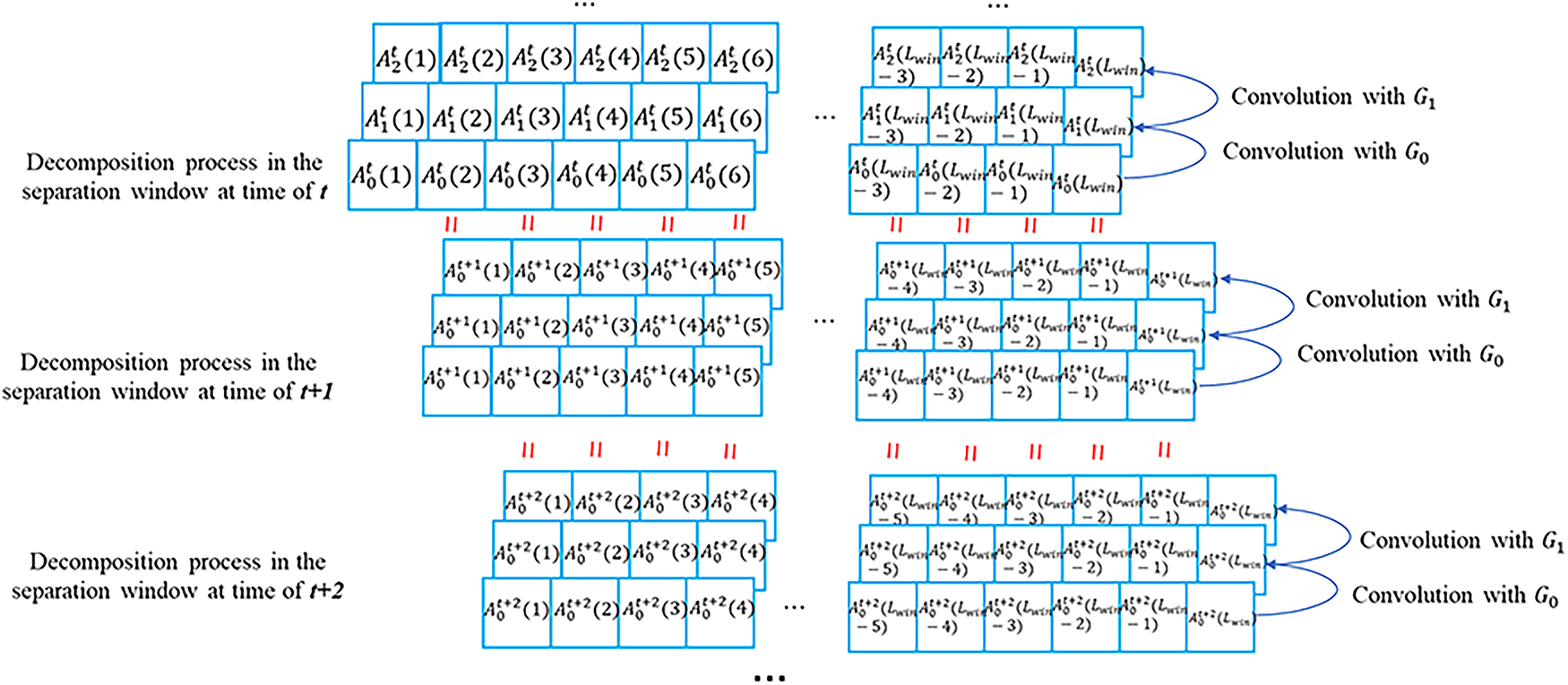
Figure 5: Process of recursive decomposition in real-time signal stream

3.1.2 Recursive Reconstruction

The nth layer of approximate signal can be obtained by downsampling (take 1 every 2n term, from the 1st term) An. In traditional DWT, each layer of reconstruction signal is convolved with the reconstruction filter after upsampling.

However, in recursive reconstruction, the first number in An and every 2n number thereafter (denoted as {a1,a2,…,ai}) are extracted to construct a new series Bn, Bn={0,0,…,0⏟2n−1zeros,a1,0,0,…,0⏟2n−1zeros,a2,…,0,0,…,0⏟2n−1zeros,ai}. Let G_o0={go1,go2,…,g_oi} (of length d), which denotes the reconstruction filter coefficient. A series of convolutional kernels G_ok (k=0,1,2,…,n−1) are constructed in the following way:

G_ok={0,0,…,0⏟2k−1zeros,go1,0,0,…,0⏟2k−1zeros,go2,…,0,0,…,0⏟2k−1zeros,g_oi},k=0,1,2,…,n−1(5)

Bn is of the same length as the original signal. Bn−1 is calculated by convolving Bn with G_on−1. Bn−2 is calculated by convolving Bn−1 with G_on−2, etc. After being downsampled by at interval of 2k, Bk is equal to the kth layer of reconstructed signal B0 is exactly the same with the reconstructed signal calculated in the Mallet algorithm.

Take the data in 3.1.1 as an example. The reconstruction filter coefficient of db1 wavelet is 22×{1,1}. So B3=223× {0, 0, 0, 0, 0, 0, 0, 1, 0, 0, 0, 0, 0, 0, 0, 44}, G_o2=22 × {0, 0, 0, 1, 0, 0, 0, 1}, G_o1=22 × {0, 1, 0, 1}, G_o0=22 × {1, 1}.

It can be calculated that B2 = 222× {0, 0, 0, 1, 0, 0, 0, 44, 0, 0, 0, 44}, B1 = 221× {0, 1, 0, 1, 0, 44, 0, 44, 0, 44, 0, 44}, B0 = {1, 1, 1, 1, 1, 44, 44, 44, 44, 44, 44, 44}, which is the same with the result calculated by the traditional method.

In real-time monitoring scenarios, from the previous section, it has been known that compared to Ant−1, Ant has the first term deleted and the rest of the terms shifted forward as a whole, adding the new input to the last term.

Since the non-zero portion of Bn consists of the integer multiples of 2nth terms in An, Bn at the time of t (denoted as Bnt) can be calculated based on Bn at the time of t−2n (denoted as Bnt−2n) by the following method: Delete the first 2n terms of Bnt−2n, add 2n−1 zeros and the last number of Ant at the end. The process is shown in Fig. 6.

Figure 6: Calculate Bnt based on Bnt−2n in real-time scenarios

In the process of calculate Bn−1t−2n from Bnt−2n, convolution is used (let the length of the convolution kernel be Lcor, Lcor=d×2n−1) and the convolution is done by adding zeros to the end of the sequence. When calculate Bn−1t from Bnt, these numbers are no longer in the end but in the middle of the sequence, causing boundary effect (will be further discussed in 3.2). So the Lcor numbers at the end of Bn−1t and the newly added 2n numbers must be recalculated, while the rest part of Bn−1t can be reused, as is shown in Fig. 7.

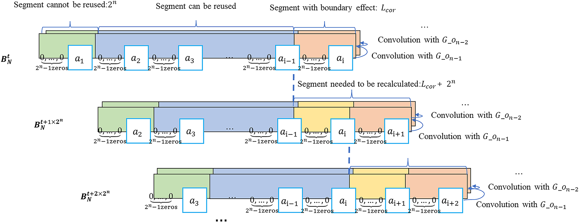
Figure 7: The reusable part of Bkt when calculating Bkt+2n

The process of getting Bn−2 from Bn−1 is similar with the method described above. It is notable that the length of the data that can be reused is still the length of the window minus Lcor+2n. B0 (the final reconstructed signal) can be calculated in this way.

Therefore, when using the recursive reconstruction method, it is necessary to use the traditional method to calculate Bn, Bn−1, …, B0 for the first 2n times. When calculating the reconstructed data when t=2n+1, refer to the data when t=1. When calculating the reconstructed data when t=2n+2, refer to the data when t=2, and so on.

So far, the framework of recursive reconstruction and the reusable part of the previous data when time forwards are clear. However, when calculating Bkt+2n based on Bkt, it is not necessary to do the convolution with G_ok. In the part that cannot be reused, only the non-zero numbers need to be figured out. Here is how the calculation can be further simplified by using a similar method in Mallet’s fast algorithm.

Firstly, the non-zero numbers to be calculated in the nth layer (the non-zero numbers in the last d×2n−1+2n numbers) are extracted (the length of these non-zero numbers is d×2n−1+2n2n=d2+1), and the zeros are inserted at interval to form a new sequence. Convolved this new sequence with the original low-pass reconfiguration filter to get the non-zero numbers to be calculated in the (n − 1)th layer. And so on until we get to layer 0, which is the final sequence of data required.

The advantage of this “pyramid” algorithm is that it uses upsampling to avoid long convolution kernel. As is shown in the figures below, the algorithm in Fig. 8 can be replaced by the one in Fig. 9. The square in the two figures represents a non-zero number and each row represents the part that needs to be recalculated in each layer.

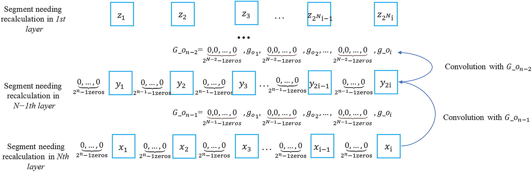
Figure 8: The original algorithm of calculating non-zero part

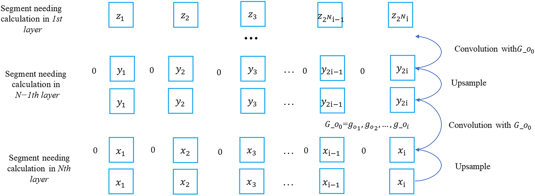
Figure 9: The improved algorithm for calculating the non-zero part

In conclusion, the flowchart of the proposed Block-wise Sliding Recursive Wavelet Transform (BSRWT) algorithm is shown in Fig. 10. The original signal is first downsampled and convolved to obtain the decomposed signal. Then, the decomposed signal is upsampled and convolved to reconstruct the separated signal. As the time window continuously slides, new segments of the original signal are input to achieve real-time signal separation. Meanwhile, data from adjacent time windows are reused to enhance the computational efficiency of the algorithm.

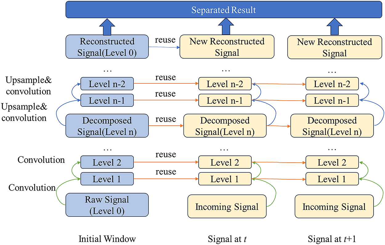
Figure 10: Flowchart of BSRWT

3.2 The Boundary Effect in Window Sliding and Its Solution

As is shown in Fig. 11, in the application of the algorithm above, the boundary of the window has a distortion effect.

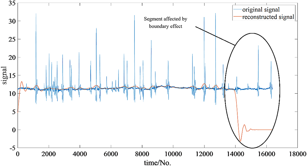
Figure 11: Boundary effect in a window

The main reasons for the boundary effect are as follows. In all the convolution processes, 0 is added to the boundary (at the start or the end of the original sequence) to ensure that the sequences before and after convolution remain of the same length. Therefore, in the process of each convolution, the way of calculation of the numbers at the beginning or the end differs from that of the numbers in the middle.

Moreover, within the section affected by the boundary effect, the degree of distortion varies. The closer to the data boundary, the more serious the distortion is. This is due to the fact that the closer to the boundary, the higher the proportion of zeros in the convolution calculation, and the greater the difference with the middle.

The main factors affecting the length of the boundary distortion are as follows. Since the distortion is caused by zeros added in the boundary in the convolution, the length of the distortion is related to the longest length of the convolution kernel used in all steps. Let the length of the decomposition and reconstruction filter be d, and the number of decomposition layers be n. In all steps of the previous methods, the longest convolution kernel is of length d×2n, so the theoretical distortion bound should be d×2n.

The boundary effect problem can generally be solved by methods like signal extension, mirroring, etc. But such methods are difficult to achieve in a scenario of real-time data stream, so in this paper a plain method is proposed as follows.

Since the boundary distortion exists at the end of each window, each time the number out of the boundary effect instead of the last number is taken as the final separation result. The cost of this is that this causes a delay of d×2n in the real-time monitoring.

3.3 Comparison between the Complexity of BSRWT and BSWT

Let the number of layers of the wavelet decomposition be n, the length of the window be Lwin=2N, and the length of the filter using the wavelet basis function be d.

When using BSWT, take a single sliding of the window as the object of study. During the decomposition process, the convolution operation of the first layer requires 2N×d multiplications, and the convolution operation of the second layer requires 2N−1×d multiplications and so on. The convolution operation of the Nth layer requires 2N−n+1×d multiplications. So a total of 2N−n+1(2n−1)×d multiplications are required to be performed in the decomposition. The wavelet reconstruction and the decomposition process require the same number of multiplication calculations. So a total of 2N−n+2(2n−1)×d multiplications are required for a single window sliding when using BSWT.

When using BSRWT, take a single sliding of the window as the object of study. During the decomposition process, d×(1+2+…+2n−1)=d×(2n−1) multiplications are required, and during the reconstruction process, d×(d2+1)×(1+2+…+2n−1)=d×(d2+1)×(2n−1) multiplications are required. So a total of d×(d2+2)×(2n−1) multiplications is required for a single window sliding when using BSRWT.

Dividing the number of multiplication calculations for the two methods yields

2N−n+2(2n−1)×dd×(d2+2)×(2n−1)=2N−n+2(d2+2)=4Lwin(d2+2)2n(6)

Overall, the computational effort of the baseline grows with the window length because each shift recomputes all convolutions inside the window, whereas the proposed method updates only boundary portions at each level; therefore, the effort per update mainly follows the number of decomposition layers and the filter length and is insensitive to the window length. Since Lwin must be strictly larger than 2n×d, BSRWT can simplify the computational complexity of BSWT in most situations, which is also well verified in the subsequent experiments.

4  Experiments and Results

4.1 Simulated Signal Experiment

The signal in the health monitoring environment is a fusion of multiple time-varying signals. In order to assess the accuracy of the above algorithms, a signal consisting of two time-varying sub-signals is simulated with reference to the previous scholars’ research [12]. BSWT and BSRWT are applied on this signal respectively to separate the time-varying sub-signals. The composition of the signal is as follows: the frequency is 50 Hz, sig1 and sig2 are both sub-signals with time-varying amplitude and frequency, sig1 is a low-frequency signal simulating non-vehicle-induced strains, and sig2 is a high-frequency signal appearing only in 25–30 s and 75–80 s, simulating vehicle-induced signals:

signal=sig1+sig2(7)

sig1=(6+0.02×sin(2πt))×cos(2πf1t)(8)

sig2=(6.3+1×sin(2πt))×cos(2πf2+π2)(9)

f1={1t<150.001×(t−30)2−225×0.001+115≤t≤451−0.001×(t−45)t>45(10)

f2={00≤t≤255×(t−30)+225≤t≤3006×(t−85)+2.5030≤t≤7575≤t≤8080≤t≤100(11)

The two signal components and the total signal after mixing are shown in Fig. 12:

Figure 12: Simulated signal for experiment

Figs. 13 and 14 show the comparison between the separation results using BSRWT and BSWT in the time and time-frequency domains under the parameter setting of db4 wavelet base and 5 decomposition layers. It can be found that the BSWT undergoes more obvious modal aliasing in the segment where the vehicle-caused signal appears, while the BSRWT gives a better result.

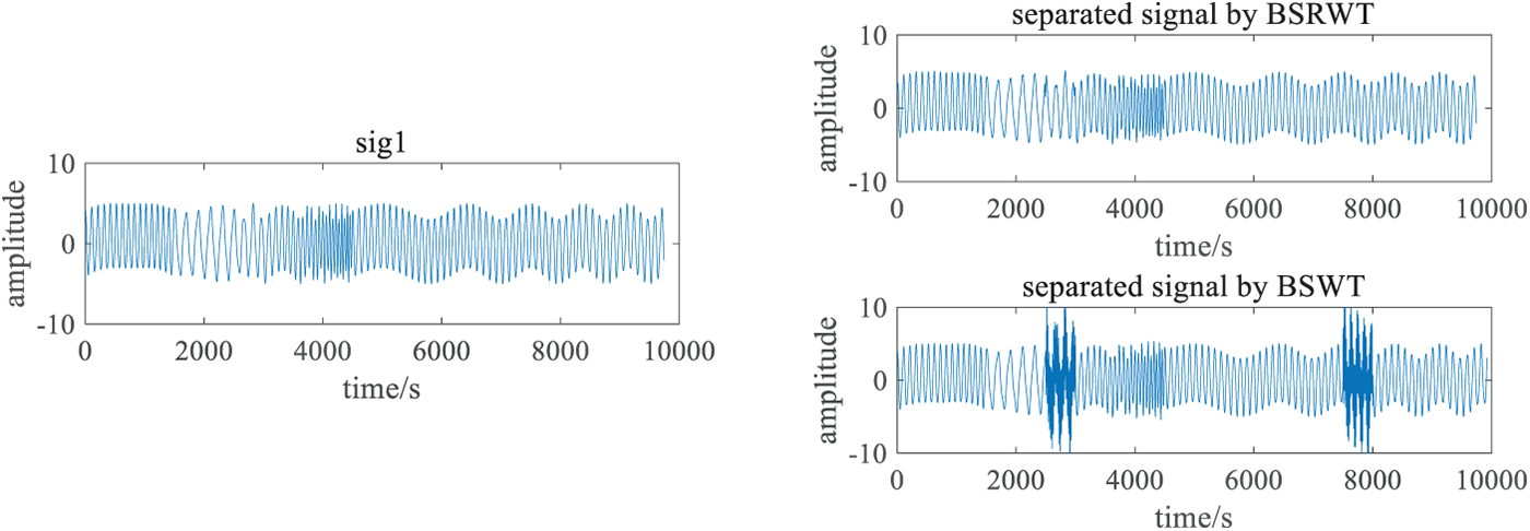
Figure 13: Time-amplitude results of BSWT and BSRWT under condition of db4, 5 layers

Figure 14: Time-frequency spectrogram of the results of BSWT and BSRWT under the condition of db4, 5 layers

To further evaluate the performance of BSWT and BSRWT under different configurations of decomposition layers, wavelet bases, and delay settings, experiments were conducted using various parameter combinations. Specifically, the number of decomposition layers was set from 1 to 5, and the wavelet basis functions were selected from ‘db2’, ‘db3’, ‘db4’, ‘db5’, and ‘db6’ for both BSWT and BSRWT to perform signal separation. For BSRWT, the delay was varied from 0 to twice the theoretical boundary length, sampled at 5-point intervals under each parameter configuration. In total, 412 sets of separation experiments were carried out using different parameter combinations.

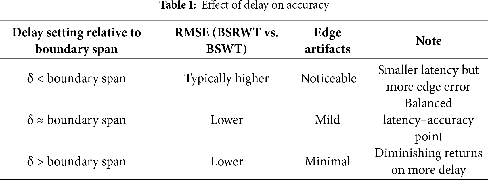
To compare the accuracy of BSRWT and BSWT under different delay settings, signal separation was performed using BSRWT with varying delays while keeping the number of decomposition layers and wavelet basis function constant. The results obtained by BSRWT were then compared with those of BSWT under the same configuration. The comparison results are presented in Fig. 15, where the horizontal axis represents the ratio of the BSRWT delay to the theoretical boundary length under the same parameter conditions, and the vertical axis represents the ratio of the RMSE of BSRWT to that of BSWT with the same decomposition layers and wavelet basis functions.

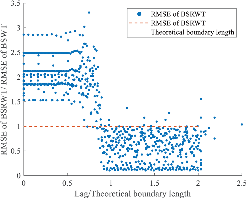
Figure 15: Result RMSE of BSRWT under different delays compared with BSWT

To investigate the accuracy of BSRWT and BSWT under different decomposition layers, the RMSE values of their separation results were calculated for each layer configuration. In the BSRWT experiments, all delay settings were chosen to be greater than the theoretical boundary length to ensure reliable separation performance. As shown in Fig. 16, samples with the same number of decomposition layers are represented by the same color. The left panel illustrates the RMSE distribution of BSRWT, while the right panel shows that of BSWT. It can be observed that, under identical decomposition layers, the RMSEs of BSRWT are consistently lower than those of BSWT, indicating that BSRWT achieves higher separation accuracy.

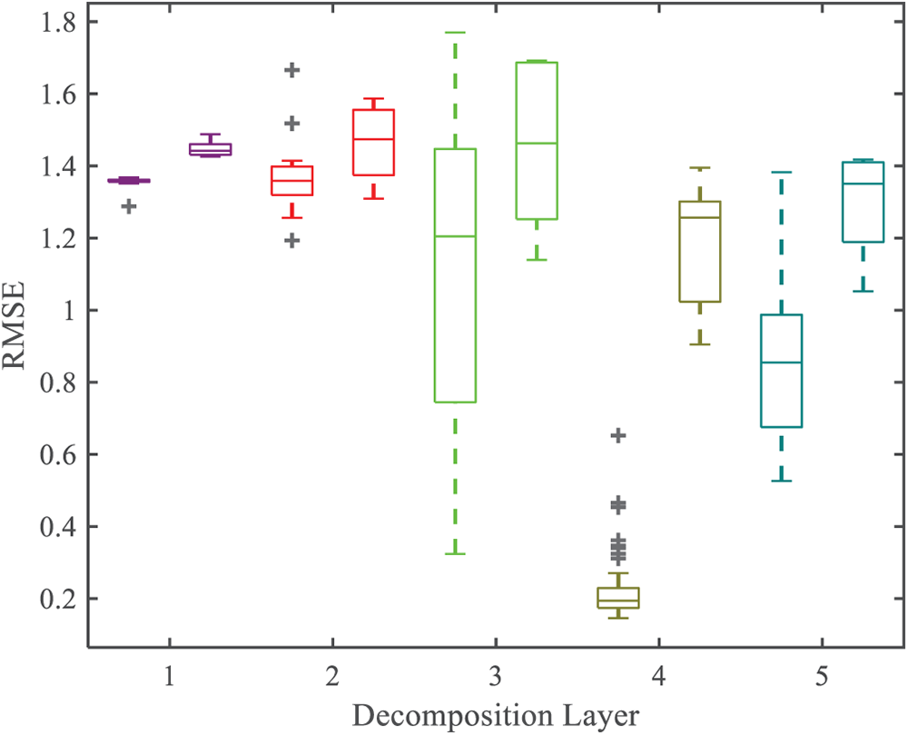
Figure 16: RMSE of BSRWT and BSWT with different decomposition layers

To examine the accuracy of BSRWT and BSWT under different wavelet bases, the RMSE values of their separation results were calculated for each wavelet basis. In the BSRWT experiments, all delay settings were greater than the theoretical boundary length to ensure consistent separation performance. As shown in Fig. 17, samples using the same wavelet basis are represented by the same color. The left panel illustrates the RMSE distribution of BSRWT, while the right panel shows that of BSWT. It can be observed that, under the same wavelet basis, the RMSEs of BSRWT are generally lower than those of BSWT, demonstrating the superior separation accuracy of BSRWT across different wavelet bases.

Figure 17: RMSE of BSRWT and BSWT with different wavelet bases

In summary, under different combinations of decomposition layers and wavelet basis functions, BSRWT demonstrates superior signal separation accuracy compared to BSWT, provided that the delay setting of BSRWT exceeds the theoretical boundary length. One possible explanation is that, although BSWT applies signal extension at the convolution boundaries to partially mitigate boundary effects, during the window-sliding process most of the separated results originate from the edge regions of the window, where signal extension still introduces residual boundary distortions, thereby reducing accuracy. In contrast, BSRWT achieves higher separation precision by incorporating information from adjacent windows, albeit at the expense of a certain processing delay.

To compare the computational complexity of the two algorithms, the elapsed time required by each method to perform signal separation under the same hardware environment and with different numbers of decomposition layers was recorded. The results are presented in Fig. 18.

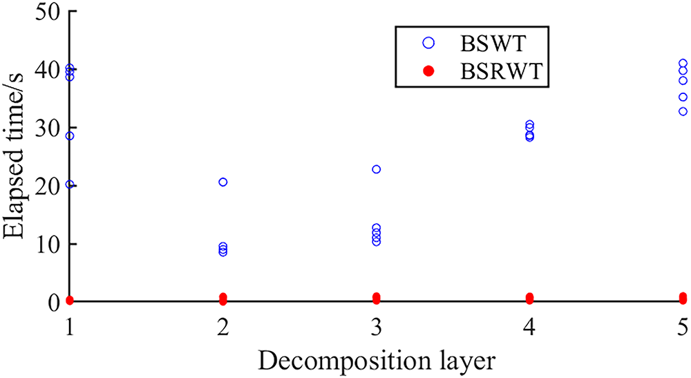
Figure 18: Elapsed time of BSWT and BSRWT under different decomposition layers

Under the same decomposition layers and wavelet basis functions, the average elapsed time of BSRWT is only 0.0249 times that of BSWT under matched settings. This provides strong evidence that BSRWT is significantly more efficient than BSWT when operating under identical parameters in real-time monitoring scenarios. In practical applications, the per-sample separation time must be shorter than the sampling period. In our field evaluation, this requirement was satisfied across all effective sampling rates listed in Table 1 (2, 4, 10, and 20 Hz), including the maximum available rate of 20 Hz.

The experimental results demonstrate that the streamlined computational complexity of the BSRWT algorithm greatly enhances the feasibility of real-time separation for high-frequency data. At the same time, BSRWT achieves substantial improvements in separation accuracy at the cost of a moderate, controllable delay. These advantages arise from a structural innovation—specifically, reusing inter-window computations and linking accuracy to a bounded, user-controlled delay—rather than from a simple implementation adjustment.

4.2 Real Strain Signal Experiment

The Lie Shi River Bridge is located on the Jiangsu Coastal Highway (Yancheng–Nantong section), crossing the Lie Shi River in Rugao City, as shown in the on-site photo in Figs. 19 and 20. The bridge superstructure consists of partially simply supported and partially continuous prestressed concrete box girders. The girder system is divided into 12 groups, each containing six spans, with a total bridge length of 2168.20 m and an average girder height of approximately 1.5 m. The bridge deck is composed of a 5 cm waterproof concrete layer overlaid with 9 cm of asphalt concrete. The health monitoring system of the Lie Shi River Bridge was commissioned in November 2015, with 56 sensors installed across key structural locations. In this study, the vertical strain signal recorded at the mid-span of the fifth span on a day in August 2018 was selected as the experimental dataset. The strain data were sampled at 20 Hz, yielding a total of 1,692,000 data points over a 24-h period.

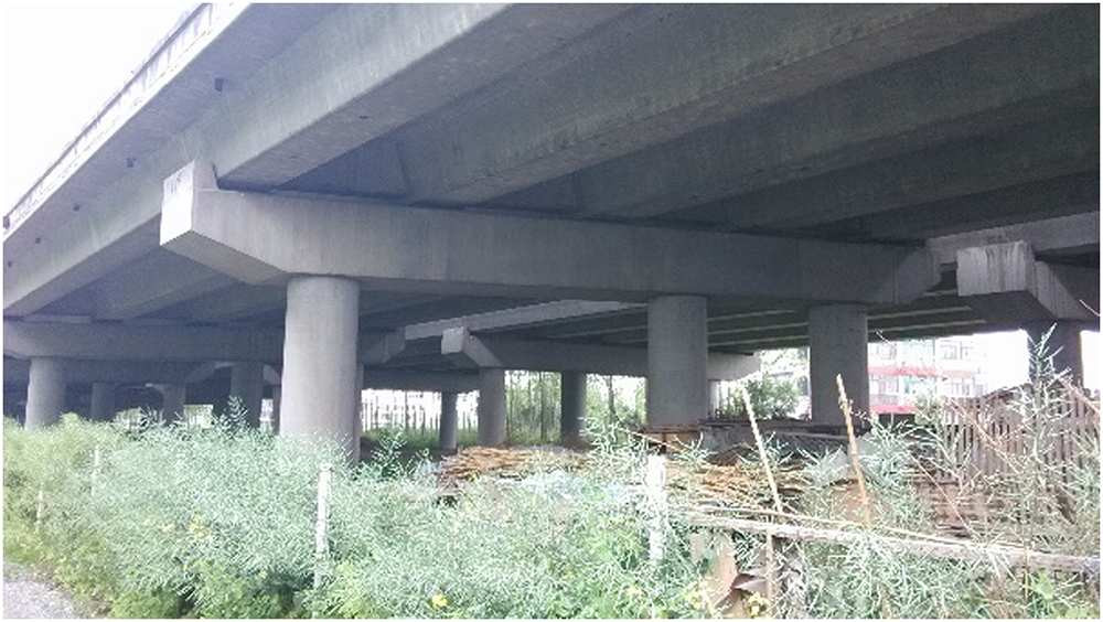
Figure 19: Field scenes of Lie Shi River Bridge

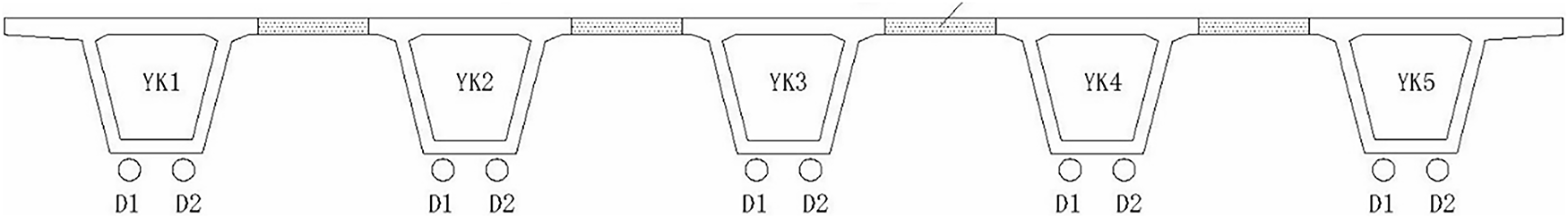
Figure 20: The section of the girder

This continuous record encompasses a wide range of typical operational conditions for long-span prestressed concrete box-girder bridges, including: (i) daily thermal cycles that drive slow drifts; (ii) mixed traffic with multi-axle trucks and time-of-day variations (nighttime low traffic vs. rush-hour high traffic), producing transient peaks with diverse amplitudes and spacings; and (iii) sensor drift and ambient disturbances. These factors jointly create the low-frequency trend plus peak-shaped transients that motivate streaming separation. The sensor is placed at the mid-span of the fifth span, a standard location for capturing vehicle-induced responses while being sensitive to thermal trends, making the case typical rather than exceptional for SHM deployments.

In separating the vehicle-induced strain from the total signal, it is necessary to remove the long-term static trend and retain the vehicle-induced component. Accordingly, separation quality can be evaluated along two dimensions: (i) the separated vehicle-induced strain should not contain long-period components, and (ii) local details of the vehicular strain should remain undistorted relative to the original signal.

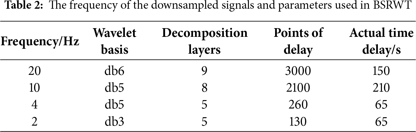
To verify the performance of BSRWT under different sampling frequencies, the original signal was downsampled to multiple target rates and processed with appropriate parameter settings. The post-downsampling frequencies and algorithm parameters are listed in Table 2. The number of decomposition layers was reduced as the sampling frequency decreased to achieve better separation, and the delay was set slightly longer than the theoretical boundary length to mitigate boundary effects.

The downsampled signals were processed using the BSRWT algorithm to obtain the long-period static strain components, which were then subtracted from the original signals to extract the vehicle-induced strain components. The separated vehicle-induced signals are presented in the following figures. Fig. 21 illustrates the original (unseparated) strain signal and its local details, while Fig. 22 displays the separated vehicle-induced signals and corresponding details under different downsampling rates. Across these sampling rates, the proposed method consistently eliminates long-period drift while preserving the peak shapes and temporal characteristics of the vehicle-induced strain. This indicates that the separation behavior remains stable and robust under varying effective sampling intervals and noise conditions within the same 24-h dataset. These findings—namely, the ability to remove slow-varying trends while maintaining transient peak integrity with bounded per-sample latency—align with the requirements of other real-time streaming signal applications such as seismic transient detection, biomedical waveform analysis, and edge IoT sensing, suggesting that the proposed approach is task-general rather than bridge-specific.

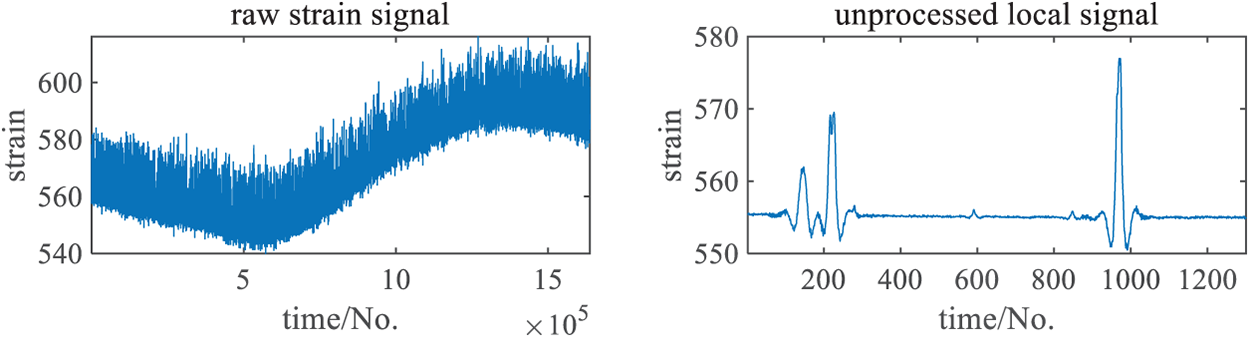
Figure 21: Unseparated signal and its local detail

Figure 22: Separated signal and its local detail at different downsampling rates

It can be observed that the unseparated signal exhibits pronounced long-period fluctuations throughout the day, primarily caused by environmental factors such as temperature variation. In contrast, this low-frequency component is effectively removed in the separated signals. A comparison of the local details between the unseparated and separated signals shows that their amplitudes and waveforms remain nearly identical, indicating that the separation process introduces no noticeable distortion to the vehicle-induced strain components.

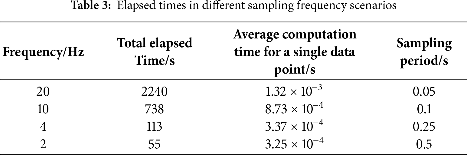
The elapsed times for the four experimental cases are presented in Table 3. In all cases, the average computation time per data point is shorter than the signal sampling period, thereby satisfying the real-time processing requirement for continuous monitoring applications.

5  Conclusion and Outlook

In this paper, a real-time vehicle-induced signal separation framework based on sliding-window wavelet decomposition is proposed and refined. The main contributions are summarized as follows:

(1) A Block-wise Sliding Wavelet Transform (BSWT) is developed for real-time signal separation. It achieves continuous separation through a sliding-window mechanism. However, its computational efficiency is limited due to redundant calculations between adjacent windows, and its accuracy is affected by boundary effects.

(2) To address these limitations, an enhanced algorithm—Block-wise Sliding Recursive Wavelet Transform (BSRWT)—is proposed. This method fully utilizes the overlapping information between adjacent windows, thereby reducing computational complexity. Meanwhile, it analyzes the origin of boundary effects and introduces an effective delay strategy to improve separation accuracy.

(3) Experiments on simulated signals demonstrate that, compared with BSWT, the improved BSRWT achieves higher separation accuracy and significantly shorter computation time, with only a minor delay introduced.

(4) Field experiments on bridge strain data further validate that the proposed method can effectively separate vehicle-induced strain from total strain, successfully removing long-term static components while preserving local waveform integrity of the vehicle-induced response.

In future work, the proposed algorithm will be further developed in the following directions. First, we plan to relax the current power-of-two window constraint, enabling support for arbitrary integer window lengths while maintaining real-time streaming capability. Second, the selection of decomposition layers and wavelet bases currently relies on empirical tuning without a theoretical foundation. We aim to establish an adaptive, data-driven selection mechanism by integrating lightweight online optimization or machine-learning–assisted strategies under bounded per-sample computational and memory costs. In parallel, we will formalize the delay–accuracy trade-off for practical applications by developing guidelines for delay adjustment in real deployments—specifically, methods for determining default delay values and strategies for increasing or decreasing the delay as noise levels or traffic conditions vary. Third, the proposed streaming framework has potential applications beyond structural health monitoring (SHM). Its deterministic updates and bounded per-sample computational complexity make it suitable for seismic monitoring (separating transient arrivals from long-period drifts under strict latency requirements), biomedical signal processing such as Electrocardiogram (ECG)/Photoplethysmography (PPG) denoising (preserving waveform morphology in on-device streaming), and Internet of Things (IoT)-based edge sensing (maintaining stable compute and memory footprints under variable sampling rates). Future studies will focus on domain-specific adaptations of layer depth and wavelet selection, followed by short-term field trials to validate the generality of the approach across different environments and sensor platforms.

Acknowledgement: The authors would like to thank all individuals and organizations that contributed to this study through administrative and technical assistance, as well as material or equipment support. Their contributions were essential to the successful completion of this research.

Funding Statement: The authors acknowledge the support of the Major Science and Technology Project of Yunnan Province, China (Grant No. 202502AD080007), and the National Natural Science Foundation of China (Grant No. 52378288).

Author Contributions: Jie Li: Writing—original draft, Visualization, Validation. Nan An: Methodology, Formal analysis, Data curation, Conceptualization. Youliang Ding: Supervision, Software, Resources. All authors reviewed the results and approved the final version of the manuscript.

Availability of Data and Materials: Data available on request from the authors.

Ethics Approval: This study involves the separation, application, and validation of bridge monitoring data. It does not involve human or animal experiments, nor the use of any sensitive materials. Therefore, formal ethical approval was not required. All experiments were conducted in accordance with standard engineering practices and safety regulations.

Conflicts of Interest: The authors declare that there is no conflict of interests in this paper.

References

1. Jayasinghe S, Mahmoodian M, Sidiq A, Nanayakkara T, Alavi A, Mazaheri S, et al. Innovative digital twin with artificial neural networks for real-time monitoring of structural response: a port structure case study. Ocean Eng. 2024;312:119187. doi:10.1016/j.oceaneng.2024.119187. [Google Scholar] [CrossRef]

2. Di Trapani F, Oddo MC, Sberna AP, La Mendola L. Structural health monitoring of masonry structures using stress sensors: experimental induced damage tests and proposed approach for real-time monitoring. Constr Build Mater. 2024;449(3):138077. doi:10.1016/j.conbuildmat.2024.138077. [Google Scholar] [CrossRef]

3. Kang G-H, Jang J, Cho G, Lee IY, Park Y-B. Real-time structural health monitoring of carbon fiber-reinforced plastic sandwich structures with carbon nanotube-dispersed core using electromechanical behavior data. Polym Test. 2024;136(1–2):108471. doi:10.1016/j.polymertesting.2024.108471. [Google Scholar] [CrossRef]

4. Jiang H, Wan C, Yang K, Ding Y, Xue S. Modeling relationships for field strain data under thermal effects using functional data analysis. Measurement. 2021;177(10):109279. doi:10.1016/j.measurement.2021.109279. [Google Scholar] [CrossRef]

5. Yang K, Ding Y, Sun P, Zhao H, Geng F. Modeling of temperature time-lag effect for concrete box-girder bridges. Appl Sci. 2019;9(16):3255. doi:10.3390/app9163255. [Google Scholar] [CrossRef]

6. Xu B, Liu C. A deep kernel regression-based forecasting framework for temperature-induced strain in large-span bridges. Eng Struct. 2025;323:119259. doi:10.1016/j.engstruct.2024.119259. [Google Scholar] [CrossRef]

7. Glashier T, Kromanis R, Buchanan C. An iterative regression-based thermal response prediction methodology for instrumented civil infrastructure. Adv Eng Inform. 2024;60(1851):102347. doi:10.1016/j.aei.2023.102347. [Google Scholar] [CrossRef]

8. Huang M, Zhang J, Hu J, Ye Z, Deng Z, Wan N. Nonlinear modeling of temperature-induced bearing displacement of long-span single-pier rigid frame bridge based on DCNN-LSTM. Case Stud Therm Eng. 2024;53(8):103897. doi:10.1016/j.csite.2023.103897. [Google Scholar] [CrossRef]

9. Wei S, Zhang Z, Li S, Li H. Strain features and condition assessment of orthotropic steel deck cable-supported bridges subjected to vehicle loads by using dense FBG strain sensors. Smart Mater Struct. 2017;26(10):104007. doi:10.1088/1361-665x/aa7600. [Google Scholar] [CrossRef]

10. Zhou Y, Sun LM, Min ZH. Girder strain analysis of a cable-stayed bridge. Zhendong Yu Chongji/J Vib Shock. 2011;30(4):230–5. [Google Scholar]

11. Zhao H, Ding Y, Li A, Ren Z, Yang K. Live-load strain evaluation of the prestressed concrete box-girder bridge using deep learning and clustering. Struct Health Monit. 2020;19(4):1051–63. doi:10.1177/1475921719875630. [Google Scholar] [CrossRef]

12. Dan D, Zeng G, Pan R, Yin P. Block-wise recursive sliding variational mode decomposition method and its application on online separating of bridge vehicle-induced strain monitoring signals. Mech Syst Signal Process. 2023;198(10):110389. doi:10.1016/j.ymssp.2023.110389. [Google Scholar] [CrossRef]

13. Dan D, Wang C, Pan R, Cao Y. Online sifting technique for structural health monitoring data based on recursive EMD processing framework. Buildings. 2022;12(9):1312. doi:10.3390/buildings12091312. [Google Scholar] [CrossRef]

14. Abrecht DG, Schwantes JM, Kukkadapu RK, McDonald BS, Eiden GC, Sweet LE. Real-time noise reduction for Mössbauer spectroscopy through online implementation of a modified Kalman filter. Nucl Instrum Methods Phys Res Sect A Accel Spectrometers Detect Assoc Equip. 2015;773:66–71. doi:10.1016/j.nima.2014.10.053. [Google Scholar] [CrossRef]

15. Ju H, Zhai W, Deng Y, Chen M, Li A. Temperature time-lag effect elimination method of structural deformation monitoring data for cable-stayed bridges. Case Stud Therm Eng. 2023;42:102696. doi:10.1016/j.csite.2023.102696. [Google Scholar] [CrossRef]

16. Wang Y, Zhang G, Wang H, Liu L, Wang X, Zheng S, et al. Investigation of temperature effects on wide steel box girder of suspension bridge based on long-term monitoring data. Sci Rep. 2024;14(1):9691. doi:10.21203/rs.3.rs-3820692/v1. [Google Scholar] [CrossRef]

17. Wang G-X, Ding Y-L, Sun P, Wu L-L, Yue Q. Assessing static performance of the dashengguan yangtze bridge by monitoring the correlation between temperature field and its static strains. Math Probl Eng. 2015;2015:1–12. [Google Scholar]

18. Chen C, Wang Z, Wang Y, Wang T, Luo Z. Reliability assessment for PSC box-girder bridges based on SHM strain measurements. J Sensors. 2017;2017(5):1–13. doi:10.1155/2017/8613659. [Google Scholar] [CrossRef]

19. Barelli L, Barluzzi E, Bidini G, Bonucci F. Cylinders diagnosis system of a 1 MW internal combustion engine through vibrational signal processing using DWT technique. Appl Energy. 2012;92:44–50. doi:10.1016/j.apenergy.2011.09.040. [Google Scholar] [CrossRef]

20. Chin C, Abdullah S, Ariffin A, Singh S, Arifin A. A review of the wavelet transform for durability and structural health monitoring in automotive applications. Alex Eng J. 2024;99:204–16. doi:10.1016/j.aej.2024.04.069. [Google Scholar] [CrossRef]

21. Chen B, Zhang Z, Sun C, Li B, Zi Y, He Z. Fault feature extraction of gearbox by using overcomplete rational dilation discrete wavelet transform on signals measured from vibration sensors. Mech Syst Signal Process. 2012;33(3):275–98. doi:10.1016/j.ymssp.2012.07.007. [Google Scholar] [CrossRef]

22. Hashim M, Nasef MH, Kabeel AE, Ghazaly NM. Combustion fault detection technique of spark ignition engine based on wavelet packet transform and artificial neural network. Alex Eng J. 2020;59(5):3687–97. doi:10.1016/j.aej.2020.06.023. [Google Scholar] [CrossRef]

23. Liu Z, Jiang B, Tang L, Liu Y, Zhang C, Li Y. Features of long-term health monitored strains of a bridge with wavelet analysis. Theor Appl Mech Lett. 2011;1(5):051006. doi:10.1063/2.1105106. [Google Scholar] [CrossRef]

24. Liu J-L, Wang S-F, Li Y-Z, Yu A-H. Time-varying damage detection in beam structures using variational mode decomposition and continuous wavelet transform. Constr Build Mater. 2024;411(4):134416. doi:10.1016/j.conbuildmat.2023.134416. [Google Scholar] [CrossRef]

25. Geetha K, Hota MK, Karras DA. A novel approach for seismic signal denoising using optimized discrete wavelet transform via honey badger optimization algorithm. J Appl Geophys. 2023;219(6):105236. doi:10.1016/j.jappgeo.2023.105236. [Google Scholar] [CrossRef]

26. Golmohammadi A, Hasheminejad N, Hernando D, Vanlanduit S, Bergh WVD. Performance assessment of discrete wavelet transform for de-noising of FBG sensors signals embedded in asphalt pavement. Opt Fiber Technol. 2024;82:103596. doi:10.1016/j.yofte.2023.103596. [Google Scholar] [CrossRef]

27. Xia Y-X, Cheng Y-F, Ni Y-Q, Jin Z-Q. A data-driven wavelet filter for separating peak-shaped waveforms in SHM signals of civil structures. Mech Syst Signal Process. 2024;219(9):111588. doi:10.1016/j.ymssp.2024.111588. [Google Scholar] [CrossRef]

28. Oh C. Application of wavelet transform in fatigue history editing. Int J Fatigue. 2001;23(3):241–50. doi:10.1016/s0142-1123(00)00091-8. [Google Scholar] [CrossRef]

29. Li S, Xu H, Zhang X, Cao M, Sumarac D, Novák D. Automatic uncoupling of massive dynamic strains induced by vehicle- and temperature-loads for monitoring of operating bridges. Mech Syst Signal Process. 2022;166(3):108332. doi:10.1016/j.ymssp.2021.108332. [Google Scholar] [CrossRef]

30. Cano A, Arévalo P, Benavides D, Jurado F. Integrating discrete wavelet transform with neural networks and machine learning for fault detection in microgrids. Int J Electr Power Energy Syst. 2024;155(3):109616. doi:10.1016/j.ijepes.2023.109616. [Google Scholar] [CrossRef]

31. de Vel O, Mallet Y, Coomans D. Chapter 4—the discrete wavelet transform in practice. In: Walczak B, editor. Data handling in science and technology. Amsterdam, The Netherlands: Elsevier; 2000. p. 85–118. doi:10.1016/s0922-3487(00)80029-5. [Google Scholar] [CrossRef]

32. Fantini D, Silva Siqueira M, Pinto M, Guimarães M, Brasil M. Wind speed short-term prediction using recurrent neural network GRU model and stationary wavelet transform GRU hybrid model. Energy Convers Manag. 2024;308(4):118333. doi:10.1016/j.enconman.2024.118333. [Google Scholar] [CrossRef]

33. Leal MM, Costa FB, Campos JTLS. Improved traditional directional protection by using the stationary wavelet transform. Int J Electr Power Energy Syst. 2019;105(9):59–69. doi:10.1016/j.ijepes.2018.08.005. [Google Scholar] [CrossRef]