Dynamic Performance of Long-Span Continuous Beam Bridges under Autonomous Truck Platooning

1  Introduction

With the rapid advancement of autonomous driving technology, autonomous truck platooning is increasingly becoming a practical reality. As an emerging transportation paradigm, platoons maintain tight formation control through vehicle-to-vehicle wireless communication, thereby reducing aerodynamic drag, improving fuel efficiency, and lowering transportation costs. Such platoons are characterized by high density, strong uniformity, and synchronized motion. When crossing bridges, these features may trigger synchronous excitation and amplify structural vibrations, potentially affecting the dynamic performance of the bridge system [1]. Compared with medium- and short-span bridges, long-span bridges can accommodate longer platoons and larger platoon sizes, leading to more complex loading scenarios. Therefore, investigating the dynamic effects of autonomous truck platooning on long-span bridges is essential for optimizing bridge design, ensuring structural safety, and prolonging service life.

Numerous scholars at home and abroad have analyzed bridge dynamic performance. According to different research methods, the literature can be divided into three main categories: finite element model analysis, experimental research, and mathematical model analysis.

Finite element models, as powerful numerical tools, are widely used to predict and analyze bridge behavior under dynamic loads. Liu et al. [2] comprehensively evaluated the static and dynamic performance of bridges by comparing static and dynamic load test results with finite element model simulation results. Li et al. [3] evaluated the dynamic response of bridges by simulating the operation of a 38-t standard truck in finite element models. Lu et al. [4] developed a finite element analysis framework based on ABAQUS for modeling dynamic vehicle–bridge interaction systems, enabling accurate evaluation of bridge dynamic performance under moving vehicle loads. Zhao et al. [5] investigated mixed traffic loading on long-span bridges using a multi-lane clustering model and found that mixed traffic flow produces significantly higher load effects than uniform traffic conditions. Tan et al. [6] conducted vehicle–bridge coupled vibration analysis to evaluate the dynamic characteristics of an arch bridge, demonstrating the effectiveness of finite element modeling in capturing bridge dynamic behavior. Ling et al. [7] investigated the influence of autonomous truck platoon loads on the dynamic amplification factor of small- and medium-span bridges. Their results indicate that such platoon loads can significantly increase the bridge’s dynamic amplification, with small-span bridges being prone to steady-state resonance, while large-span bridges are more susceptible to transient resonance.

Experimental research is key to validating the accuracy of theoretical analysis and numerical models. Song et al. [8] used support vector machine methods combined with measured data of vehicles operating on bridges to establish a system for predicting bridge dynamic performance. Li et al. [9] studied the effects of factors such as vehicle speed, lane position, and weight on bridge dynamic response through field experiments, providing empirical data for understanding bridge behavior under actual traffic loads. Kaloop et al. [10] used short-term non-destructive structural health monitoring systems to conduct real-time evaluation of bridge dynamic performance by changing truck position and speed. These monitoring data are valuable for revealing the dynamic characteristics of bridges in actual operation. Yang et al. [11] analyzed the impact of single vehicles in non-moving and moving states on bridges through bridge simulation experiments.

With the development of computational technology, establishing mathematical models to understand the interaction between vehicle loads and bridge dynamic response has also become a new approach. Obrien et al. [12] obtained various vehicle parameter information using WIM systems and provided new perspectives for solving the dynamic response of highway bridges under single vehicle loads through statistical analysis of these parameters. Mo et al.’s [13] research advanced the dynamic analysis of vehicle–bridge interaction systems by incorporating coherent road roughness, multiple-lane excitation, and time-varying interpolation effects. Zhang et al. [14] analyzed vehicle ride comfort based on a vehicle–bridge coupled vibration model, further demonstrating the applicability of coupled dynamic analysis for evaluating bridge–vehicle interaction responses. Generally, road roughness [15], bridge structure type, vehicle speed, axle load, wheelbase, and vehicle suspension parameters affect the bridge’s dynamic performance [16–18]. Ma et al. [19] developed a dynamic analysis model of vehicle platoons and continuous beam bridges through numerical simulations, and systematically investigated the effects of factors such as vehicle speed and vehicle spacing on the bridge’s dynamic amplification factor.

In summary, although studies on the dynamic response of bridges under vehicular loading are relatively well established, existing research has predominantly focused on single-vehicle loads or stochastic traffic flows. Systematic investigations of autonomous truck platoon loading, particularly considering their inherently high synchrony, are still notably lacking. Autonomous truck platoons impose highly clustered, synchronized, and strongly time-varying excitations on bridges, exhibiting dynamic characteristics that differ substantially from those of conventional traffic loads and potentially inducing complex coupled vibration effects. Moreover, most existing studies emphasize single-factor sensitivity analyses, lacking a comprehensive quantitative evaluation of the interactions among key variables such as vehicle speed, number of formations, vehicle spacing, and vehicle weight. These research gaps are particularly pronounced for long-span continuous beam bridges.

To address the above research gaps, this study investigates a large-span continuous beam bridge by establishing a vehicle–bridge coupled dynamic model and employing a mixed-level orthogonal experimental design. The effects of vehicle speed, number of formations, vehicle spacing, and vehicle weight—as well as their interactions—on mid-span deflection and dynamic amplification factors are systematically analyzed. The objective is to elucidate the dynamic response mechanisms under multi-factor coupling, identify the critical parameter combinations that lead to amplified dynamic effects, and propose operational control recommendations for truck platoons on large-span bridges. The findings provide a theoretical basis for parameter optimization of autonomous truck platoons, bridge operational safety assessment, and future enhancements to design specifications.

2  Formation Load Form

Formation load is a unique type of bridge load that involves a group of vehicles moving across the bridge. Researchers have investigated the impact of these vehicle groups on bridges. Hulaseedharan and Yarnold [20] examined 24 different truck platoon scenarios to assess their effects on bridge load levels. He simulated various vehicle spacing and formation sizes and found that the load level increases with the span length. Tohme and Yarnold [21] used the FDOT C5 truck model to study how different formation sizes and vehicle spacing affect bridges. He also evaluated the performance of bridges designed according to the AASHTO HL-93 standard. Ling et al. [22] analyzed the load effects of automated truck platooning on highway bridges and demonstrated that vehicle spacing, platoon size, and platoon configuration significantly affect bridge load demands.

Based on the literature review, the standard vehicle adopted in this study is the three-axle truck specified in the American vehicle load specification [23]. The axle loads of the three axles are 35, 145, and 145 kN, respectively, with a total gross weight of 325 kN. The configuration of the selected standard three-axle truck is illustrated in Fig. 1.

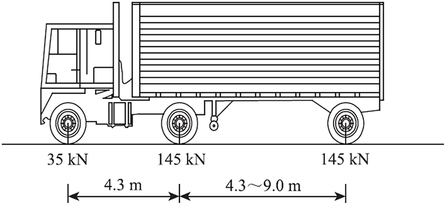
Figure 1: Standard vehicle model diagram

To simulate the dynamic interaction during vehicle passage over the bridge, this study adopts a lumped mass–spring–damper model to construct the dynamic system of a three-axle vehicle. The vehicle body mass, axle masses, and suspension system are respectively represented by equivalent mass blocks and spring–damper elements. The vehicle–bridge interaction is realized through contact elements between the wheel nodes and the bridge deck nodes, while the vertical wheel loads are applied as time-varying, multi-axle concentrated forces moving along the bridge surface. This modeling approach effectively captures the influence of axle loads, suspension stiffness, and damping parameters on the bridge’s dynamic response, while maintaining high computational efficiency, making it suitable for dynamic analysis of synchronized multi-vehicle platoons.

In the dynamic analysis, the vehicles are assumed to travel along the bridge deck at a constant speed, while the longitudinal flexibility and pitching degrees of freedom of the vehicle body are neglected. Under this assumption, the vehicle loads acting on the bridge can be simplified as a time-varying sequence of vertical wheel loads. The suspension system is modeled using linear spring–damper elements, and the contact stiffness between the tires and the bridge deck is set to 4.87 × 106 N/m [24], a commonly adopted parameter in vehicle–bridge coupled dynamic analyses. This simplified model maintains the required computational accuracy while significantly improving computational efficiency, making it particularly suitable for high-frequency loading scenarios involving multi-vehicle platoons.

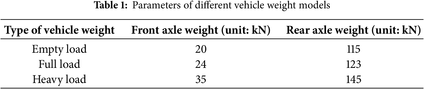
According to the provisions of the Limits of Dimensions, Axle Load and Masses for Motor Vehicles (GB 1589-2016) [25], the maximum allowable gross mass for a three-axle truck is 25–27 t (approximately 250–270 kN). This limit is intended to ensure that the load imposed by vehicles does not exceed the design load-carrying capacity specified in the Specifications for Design of Highway Reinforced Concrete and Prestressed Concrete Bridges and Culverts (JTG 3362-2018) [26]. By restricting excessive axle loads, the code aims to prevent excessive deflection, cumulative structural fatigue, and potential safety risks, thereby ensuring the structural safety and durability of bridges during service. Considering the weight ranges of three-axle trucks specified in Chinese and U.S. standards, as well as commonly adopted settings in platoon-load studies, this study classifies vehicle loading conditions into three categories—empty load, full load, and heavy load. The corresponding axle load configurations are listed in Table 1.

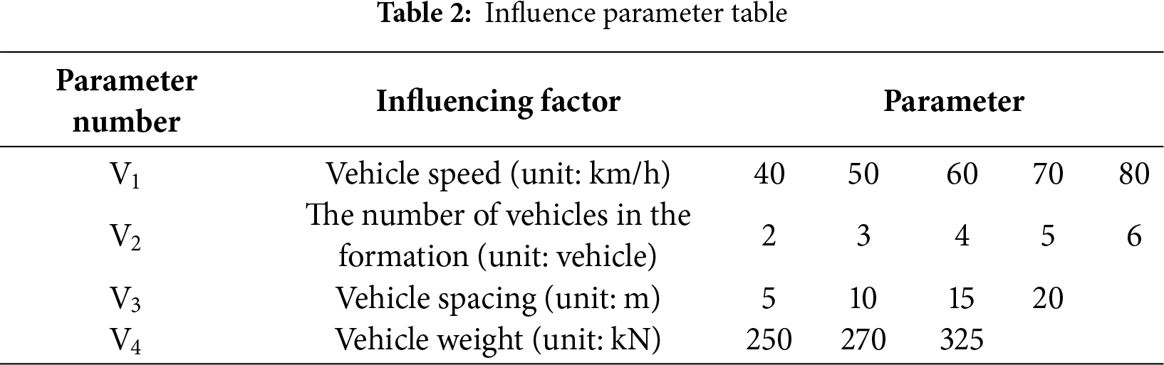
In autonomous truck platoon operations, vehicles maintain tightly coordinated motion through wireless communication and onboard sensing technologies, enabling stable and precise short vehicle spacing even at relatively high speeds. As a result, vehicle speed, number of formations, vehicle spacing, and vehicle weight constitute the four primary parameters governing platoon-induced dynamic loads on bridges. To ensure that the parameter ranges adopted in this study are both representative of realistic operating scenarios and consistent with relevant regulatory and technical constraints, the parameter selections were determined based on typical highway operating conditions, the functional capabilities of current autonomous platoon systems, and applicable national and international standards.

Specifically, the vehicle speed is set to 40–80 km/h, a range that encompasses medium-speed conditions frequently encountered on climbing sections, congested segments, and bridge approaches, as well as the upper speed limit for heavy trucks prescribed in China and many other jurisdictions. This choice allows the study to capture the transition of bridge dynamic responses from moderate to high-speed excitation. The number of formations is defined as 2–6 vehicles. The lower bound corresponds to the minimum requirement for forming a platoon, while the upper bound reflects the scale commonly adopted in current autonomous platooning pilot programs, considering constraints related to communication latency, traffic interaction, and platoon management safety.

The vehicle spacing is set to 5–20 m, covering high-density spacing achievable by advanced Cooperative Adaptive Cruise Control systems (approximately 5 m), as well as more conservative or degraded-mode spacing (approximately 20 m) that provides a practical baseline for comparison. Vehicle weight is classified into empty-load (≈250 kN), full-load (≈270 kN), and heavy-load (≈325 kN) categories. The empty- and full-load classes correspond to the maximum allowable gross mass (25–27 t) for three-axle trucks specified in the Limits of Dimensions, Axle Load and Masses for Motor Vehicles (GB 1589-2016), while the heavy-load class corresponds to the standard design truck adopted in the AASHTO specifications, enabling evaluation of bridge safety margins under heavy-duty conditions.

Overall, these parameter ranges comprehensively represent the major operational scenarios of autonomous truck platoons and provide a robust basis for investigating the multi-factor effects on bridge dynamic responses. To improve the clarity and consistency of subsequent analyses, the four influencing factors listed in Table 2 are uniformly denoted as standardized variables V1–V4. This notation facilitates concise presentation in later sections.

To illustrate how vehicle loads are applied in the model, Fig. 2 presents an example of the axial load distribution for a platoon consisting of three heavy-load trucks with a 10 m inter-vehicle spacing traveling along the longitudinal centerline of the bridge deck. This figure demonstrates the movement of multi-axle wheel loads along the bridge over time, providing an intuitive basis for the subsequent transient dynamic analysis.

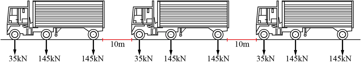
Figure 2: Truck formation load diagram

3  Dynamic Model

3.1 Analysis Principle of Dynamic Model

This study employs a transient dynamic analysis to evaluate the bridge’s dynamic response under autonomous truck platoon loading. Transient dynamics can fully capture the structural response throughout the entire process of time-varying and non-periodic moving loads, making it particularly suitable for scenarios involving the highly synchronized, multi-axle continuous excitations and strong temporal variability characteristic of autonomous truck platoons. Compared with steady-state or modal superposition methods, transient analysis provides a more accurate representation of short-duration impact effects and peak responses arising from vehicle–bridge interactions; therefore, it is adopted as the dynamic solution method in this study.

The equation of motion of the structure under dynamic loading can be expressed as the standard second-order vector differential form, as shown in Eq. (1):

Mu⋅⋅(t)+Cu⋅(t)+Ku(t)=F(t),(1)

where M is the mass matrix, C is the damping matrix, K is the stiffness matrix, u is the nodal displacement vector, u⋅ is the nodal velocity vector, u⋅⋅ is the nodal acceleration vector, and F(t) is the time-dependent external load vector.

In finite element software environments, transient dynamic analysis can be implemented using various approaches, including the direct method, modal superposition method, and reduction techniques, each characterized by distinct theoretical foundations and applicability. The direct method solves the structural dynamic equilibrium equations while retaining all degrees of freedom, and obtains the full time-history responses of displacement, velocity, and acceleration through implicit integration schemes such as the Newmark−β method. This approach simultaneously accounts for the coupled effects of the mass, damping, and stiffness matrices, offering the highest accuracy and applicability under strongly nonlinear behavior, broadband excitation, and time-varying loads. It is therefore the most comprehensive and reliable solution strategy for transient dynamic analysis. The modal superposition method extracts the dominant lower-order modes of the structure and solves the dynamic response in modal coordinates, thereby significantly reducing computational effort. However, this method relies on the assumption of system linearity and fails to accurately capture structural time-history responses when subjected to multi-vehicle platoon loading, broadband excitation, or conditions where higher-order modes contribute significantly. Reduction techniques further decrease the computational scale by condensing the degrees of freedom, but at the cost of suppressing higher-order modes and local dynamic behaviors. As a result, they are unsuitable for complex loading scenarios such as truck platoon excitations, which involve high-frequency components and strong temporal variability.

Considering that platoon loading is characterized by high-density axle loads, broadband excitation, and strong synchrony, the direct method is adopted in this study to perform the transient dynamic analysis in order to achieve higher computational accuracy.

Time integration is carried out using the Newmark−β implicit integration algorithm, in which the parameters γ and β are introduced to approximate acceleration and velocity within each time step. The velocity and displacement update formulas are given in Eqs. (2) and (3):

un+1=un+Δtun⋅+Δt2((12−β)un⋅⋅+βun+1⋅⋅),(2)

un+1⋅=un⋅+Δt((1−γ)un⋅⋅+γun+1⋅⋅),(3)

In these equations, un represents the displacement at time step n, and un+1 represents the displacement at time step n+1. Similarly, un⋅ and un+1⋅ denote the velocities at time steps n and n+1, respectively, while un⋅⋅ and un+1⋅⋅ correspond to the accelerations at time steps n and n+1. Term Δt denotes the time increment Δt between two successive time steps. The parameter β controls the weight of the acceleration term in the displacement update, and γ controls the contribution of the acceleration term in the velocity update. Setting γ=0.5 and β=0.25 ensures numerical stability under the high-frequency excitations induced by vehicle platoons. A time step of 0.001 s is adopted in this study to accurately capture the rapid response variations as each axle group traverses the bridge. All computations are conducted in the ANSYS Mechanical 2024R1 environment to ensure consistency in solver settings and modeling procedures.

The bridge structure is modeled using SOLID185 three-dimensional solid elements to establish a finite element model of a three-span continuous box girder with spans of 75 m + 120 m + 75 m. Material parameters are assigned according to the Specifications for Design of Highway Reinforced Concrete and Prestressed Concrete Bridges and Culverts (JTG 3362-2018), assuming that the concrete follows a linear elastic constitutive relationship. The vehicles are represented by a lumped mass–spring–damper model for three-axle trucks, with the axle loads applied through contact elements connected to the bridge deck nodes, thereby enabling dynamic coupling between the vehicles and the bridge. The vehicles move at a prescribed constant speed along the centerline of the bridge deck, and the multi-axle wheel loads act sequentially on the deck nodes as functions of time, forming a continuous moving load.

3.2 Dynamic Analysis Process

The workflow for transient dynamics analysis typically consists of three stages: preprocessing, solving, and postprocessing.

In the preprocessing stage, the establishment of geometric models, definition of material properties, and construction of finite element models are key steps, whose accuracy has a decisive impact on the accuracy of subsequent analysis results. In this stage, we first establish the geometric model of the bridge, including the shape and dimensions of the main beam, ensuring consistency with the actual structure. Then, we define the mechanical properties of materials for the bridge, such as elastic modulus and density, which directly affect the structural response. Next, we apply boundary conditions, including the positions of supports and constraints, to simulate actual working conditions. Finally, we perform mesh generation to create discrete elements for numerical analysis, where mesh quality directly affects the accuracy of numerical analysis. During the mesh generation process, special attention must be paid to mesh density in critical areas to ensure the accuracy of numerical simulation.

The solution phase involves applying displacement and load boundary conditions, setting solution parameters, and selecting appropriate numerical integration methods. In this phase, the solution type was configured for transient dynamic analysis with relevant parameters. Displacement boundary conditions were applied to the structure. Subsequently, vehicle loads were applied at specific locations on the structure, including vehicle speed, vehicle spacing, weight, and number of formations, to simulate the effects of vehicle loads on the bridge. Finally, numerical integration calculations were performed to obtain the bridge response under load action.

The post-processing phase focuses on analyzing computational results to ensure their reliability and validity. In this phase, we primarily analyzed the deformation conditions at the mid-span of the bridge’s middle span and the most unfavorable deformation conditions of the side spans, and evaluated whether the deformation distribution met expectations. The workflow of the transient dynamic analysis is illustrated in Fig. 3.

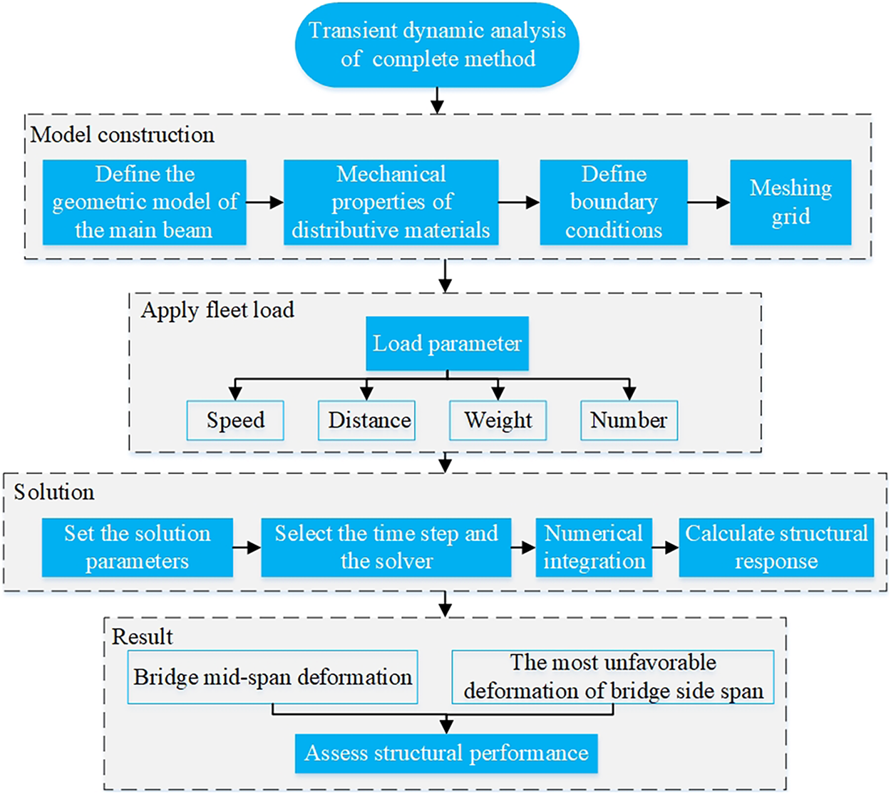
Figure 3: Transient dynamic analysis flow chart

Through this analysis process, this study deeply reveals the response characteristics of bridge structures under dynamic loads, and provides a solid scientific basis for bridge design and performance evaluation.

4  Case Analysis

4.1 Engineering Background

In this paper, a continuous box girder bridge on a highway is selected as the research object to construct the model. The bridge is a prestressed concrete continuous box girder with variable height, and the span combination is 75 m + 120 m + 75 m. The central beam height of the box girder at the middle fulcrum is 6.7 m, and the central beam height of the mid-span box girder is 2.8 m. The transition section of the beam height is adjusted by the height of the inner and outer webs of the box girder, and the beam height changes with a quadratic parabola. In this study, the prestressed concrete box girder structure adopted has the characteristics of single box and single room section. The specific geometric parameters are as follows: the bottom width of the box girder is 7 m, and the total width is 13.5 m. The thickness of the roof is 0.28 m, the thickness of the end of the cantilever plate is 0.18 m, and the thickness of the root is 0.8 m. The thickness of the web varies from 0.45 to 0.70 m, and the thickness of the bottom plate varies from 0.28 to 0.85 m. The diaphragms are set at the middle fulcrum, the side fulcrum and the middle span of the middle span, and their thicknesses are 1.6, 1.9 and 0.5 m, respectively. The concrete design strength of the prestressed concrete box girder structure is 50 MPa.

The prestressed steel strand is selected according to ASTM A416-97 standard, and its standard strength grade is 1860 MPa. The elastic modulus of steel strand is 1.95 × 105 MPa. In the process of prestressed tension, the control stress σK under the anchor is calculated according to 0.72 times the allowable stress R, and the value is 1339.2 MPa to ensure the safety and functionality of the structure. The elevation of the continuous box girder bridge is shown in Fig. 4, while the cross-sections of the box girder are illustrated in Fig. 5a,b.

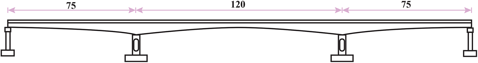
Figure 4: Elevation drawing of a 75 + 120 + 75 m prestressed concrete continuous box girder bridge (unit: m)

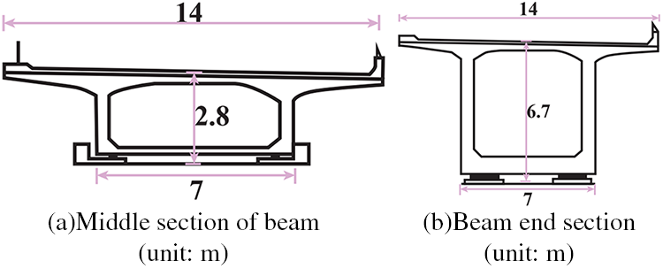
Figure 5: Section drawing of a 75 + 120 + 75 m prestressed concrete continuous box girder bridge

4.2 Dynamic Model Establishment

According to the parameters of the engineering background bridge, the solid element model can be constructed in the finite element software. The element type is SOLID185, the number of elements is 18,254, the number of nodes is 30,849, and the material property is set to C50 concrete. The 1:1 concrete continuous box girder bridge model is shown in Fig. 6.

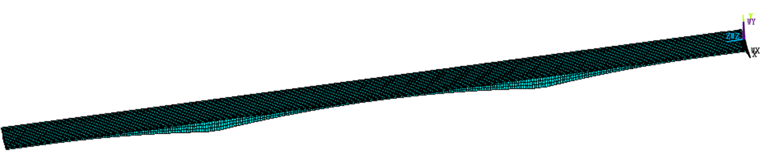
Figure 6: Bridge finite element model

To verify the reliability of the model, this study compares the theoretical mid-span deflection under code-specified loading conditions with the numerical results obtained from the finite element model. For a three-span continuous beam, the theoretical mid-span deflection under the combined uniformly distributed load and concentrated load is calculated using Eq. (4):

Δ=qkL4K1EI+PkL3K2EI,(4)

where qk represents the uniformly distributed load, Pk the concentrated load, L the span length, K1 and K2 the deflection coefficients for continuous beams, E the elastic modulus of concrete, and I the equivalent moment of inertia of the mid-span cross-section.

According to the General Specifications for Design of Highway Bridges and Culverts (JTG D60-2015) [27], the values of qK=10.5 kN/m and PK=360 kN can be obtained, and the calculated mid-span deflection is 4.74 cm. The finite-element simulation yields a deflection of 4.72 cm, which falls within the allowable engineering error range; therefore, the model is considered reliable for subsequent analyses.

4.3 Orthogonal Test

Orthogonal experimental design is a statistical method widely used in multi-factor studies. By constructing carefully arranged test schemes, it enables a systematic investigation of the combined effects of multiple factors and their different levels on the response of interest. The key advantage of this method lies in its ability to comprehensively evaluate the overall influence of several factors and to reveal potential interactions among them with a relatively small number of test runs.

According to the principles of orthogonal design and the variables considered in this study, vehicle speed is set at five levels, number of formations at five levels, vehicle spacing at four levels, and vehicle weight at three levels. The specific factor levels used in the orthogonal design are summarized in Table 3.

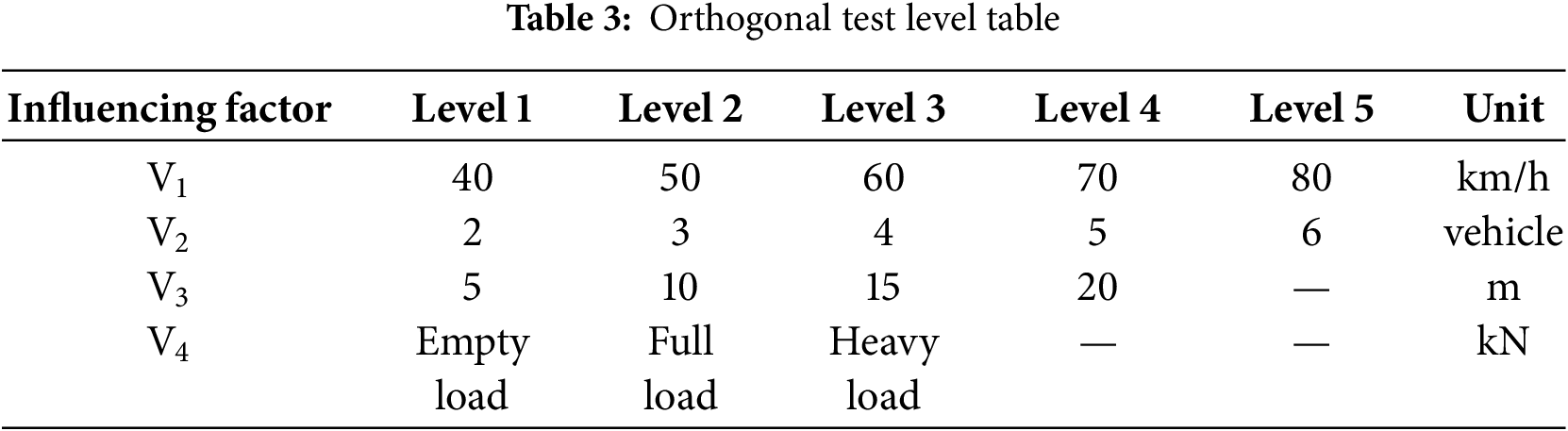
Considering the number of levels for vehicle speed and number of formations, the L25(5^5) orthogonal table can be selected, which can accommodate 5 five-level factors. However, since the levels of vehicle spacing and vehicle weight are not 5, the selection of orthogonal table needs to be adjusted.

According to the basic theory of mixed orthogonal arrays, an orthogonal array with mixed levels can be selected. When constructing an orthogonal design suitable for mixed multi-level factors, the test matrix must be systematically designed based on the characteristics of the variables and the underlying mathematical principles. For the asymmetric multi-level system composed of vehicle speed (five levels), number of formations (five levels), vehicle spacing (four levels), and vehicle weight (three levels), according to the degrees-of-freedom requirement in orthogonal experimental design, the minimum number of required tests can be determined using Eq. (5):

∑i=14(mi−1)=2×(5−1)+(4−1)+(3−1)=13(total degrees of freedom),(5)

Accordingly, the lower bound of the required number of tests is derived as N ≥ 14. Based on an adaptability analysis of available orthogonal arrays, several conventional schemes are excluded, including L25(56) (non-mixed structure), L36(3¹² × 2¹²) (level-dimension mismatch), and L50(5¹0 × 25) (excessive proportion of two-level columns).

To address the coexistence of the three-level factor (vehicle weight) and the four-level factor (vehicle spacing), the pseudo-level technique proposed by Hu [28] is employed for column reconstruction. Specifically, the three original levels {1, 2, 3} of vehicle weight are expanded into a four-level column {1, 2, 3, 3} through a level-overlay strategy. This operation satisfies the E(s²) minimization principle (variance inflation factor VIF = 1.18, p > 0.05), while preserving the native four-level structure of the vehicle spacing factor. Following a search of international orthogonal array libraries and verification of orthogonality, the array L44(44 × 54) is identified as the optimal solution.

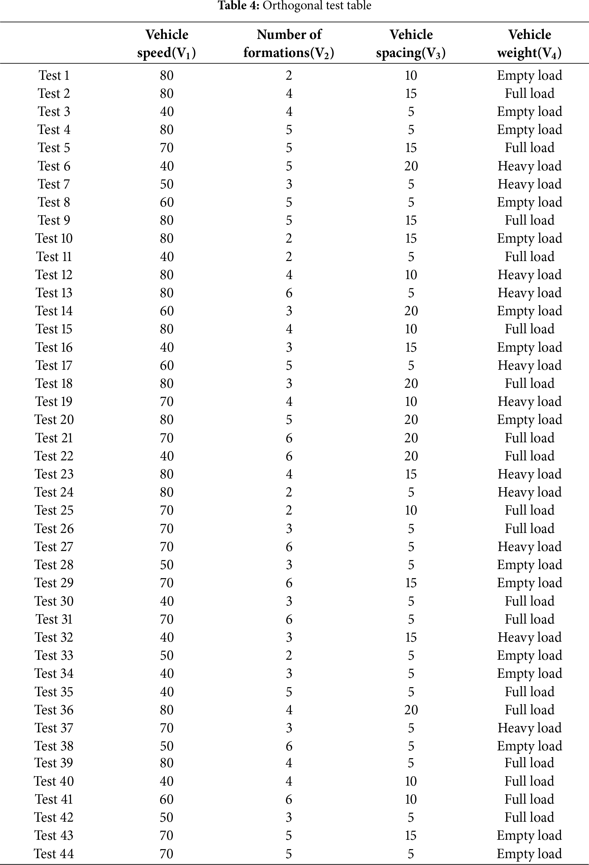
Based on the principles of orthogonal experimental design, the final orthogonal test matrix for the target variables is constructed as shown in Table 4.

4.4 Experiment Results and Analyses

According to the content of the orthogonal test table, the deformation and dynamic coefficient of the bridge span are obtained, see Table 5. The dynamic coefficient is the ratio of the maximum response of the structure under dynamic load to the maximum response of the structure under the same load static action.

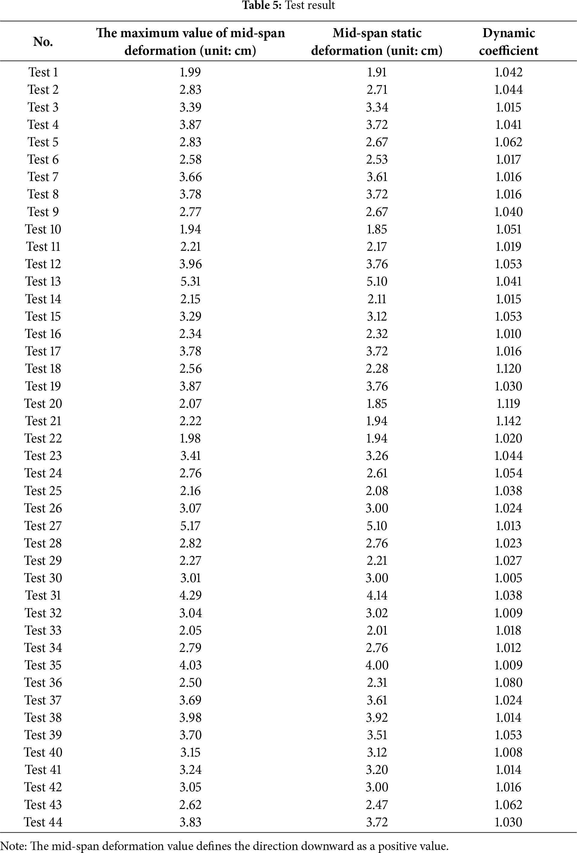
The experimental results in Table 5 show that the bridge dynamic amplification factors range from 1.01 to 1.14. To systematically reveal the influence patterns of the various factors and their interactions on the dynamic amplification factor, this study first conducts a correlation analysis, followed by interaction plots to examine significance trends, and finally performs an analysis of variance (ANOVA) to quantitatively investigate the underlying interaction mechanisms.

(1) The correlation between different influencing factors and the dynamic performance of the bridge.

Firstly, the correlation analysis between different influencing factors and the dynamic performance of the bridge is carried out. Considering the non-linear and non-normal distribution characteristics of each group of test data and the limited number of test samples, we used Spearman correlation coefficient to analyze the relationship between the data. The results of correlation analysis are shown in Fig. 7. The analysis results intuitively reveal the correlation intensity and direction between different elements.

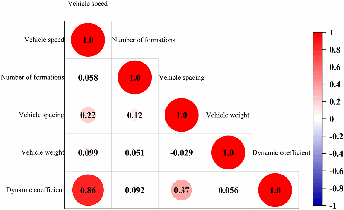
Figure 7: Spearman correlation coefficient diagram between elements

According to Fig. 7, the correlation coefficients between vehicle speed and vehicle spacing with the bridge dynamic coefficient are 0.86 and 0.37, respectively, indicating significant positive correlations for both factors, with vehicle speed exerting a particularly strong influence. In contrast, the correlation coefficients for the number of formations and vehicle weight are only 0.092 and 0.056, suggesting that these two factors have relatively minor impacts on the dynamic coefficient. To further reveal the potential nonlinear coupling relationship among vehicle speed, vehicle spacing, and dynamic coefficient, we constructed a three-dimensional bubble chart where the number of formations represents bubble size and vehicle weight class is color-coded. Additionally, we created schematic diagrams illustrating the impact points on bridges for vehicle formations at different vehicle spacing. These visualizations are presented in Figs. 8 and 9.

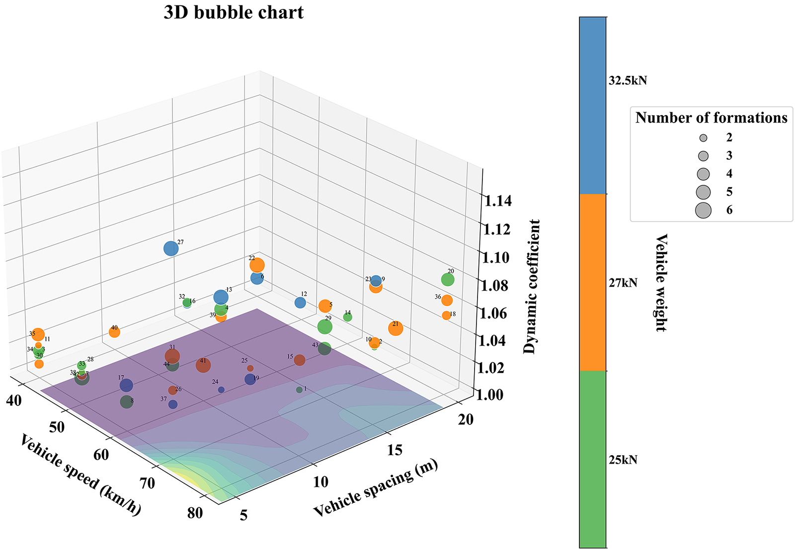
Figure 8: Three-dimensional bubble chart of vehicle speed, vehicle spacing, and dynamic coefficient

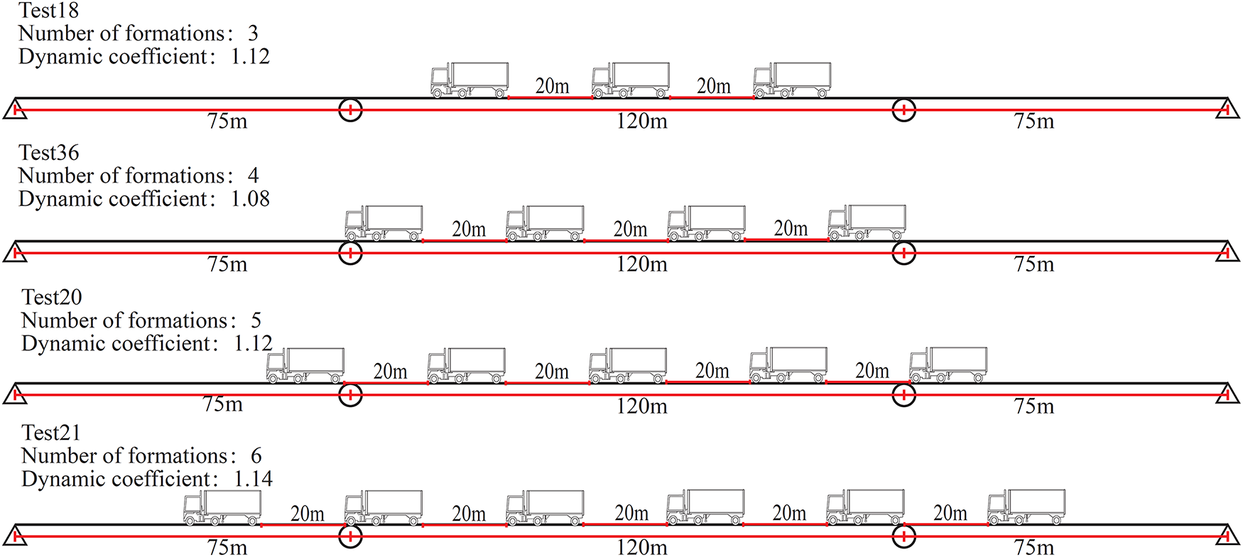
Figure 9: The schematic diagram of the influence point of vehicle formation on the bridge under different vehicle spacings

Observing Fig. 8, it can be found that under most operating conditions, the influence range of vehicle speed and vehicle spacing on the dynamic coefficient is between 1.01 and 1.06. However, when vehicle speed is high, the dynamic coefficient generally exceeds 1.06, indicating that vehicle speed is the primary factor affecting the dynamic coefficient. Furthermore, as the number of vehicles in the platoon increases, the mid-span deformation of the bridge shows an overall upward trend and is generally higher than conditions with fewer vehicles in the platoon. However, under certain conditions, such as when vehicle spacing is small, the influence of increased number of formations on mid-span deformation weakens, and deformation values are relatively reduced. This indicates that the reduction in maximum mid-span deformation exceeds the static deformation at mid-span, resulting in a decrease in the dynamic coefficient [29]. Particularly, under conditions of 50 km/h vehicle speed with 5 m spacing, and 60 km/h vehicle speed with 5 m spacing, the dynamic coefficient shows a trend of first decreasing then increasing as number of formations increases. The mechanism can be explained as follows: when number of formations is small, the vehicle platoon forms a significant concentrated load distribution, leading to increased mid-span deformation and dynamic coefficient; as number of formations increases, load distribution tends to become dispersed, the concentration effect in the mid-span region weakens, and the maximum deformation and dynamic coefficient correspondingly decrease. This phenomenon indicates that the combined effect of number of formations and load distribution patterns, under certain conditions, can have non-monotonic impacts on structural dynamic response. For example, in Tests 4 and 20, despite having the same vehicle speed and number of formations (both 5 vehicles), the increased vehicle spacing leads to platoon dispersion, which reduces the concentrated loading effect on the bridge, resulting in a decreased bridge dynamic coefficient. Fig. 9 shows a schematic diagram of the influence of vehicle spacing on the bridge.

(2) Main effect analysis of influencing factors

Based on the results of the preliminary analysis described above, we further conducted main effects analysis for various influencing factors. The corresponding results are shown in Figs. 10–12. Interaction plots illustrate the variation trends of the dynamic amplification factor under different combinations of factor levels, allowing the strength and nature of interaction effects to be assessed. In general, pronounced crossings of the factor-level lines in the plots indicate significant interaction effects [30]. This analytical method helps us better understand how various factors collectively influence changes in bridge dynamic coefficients under different conditions.

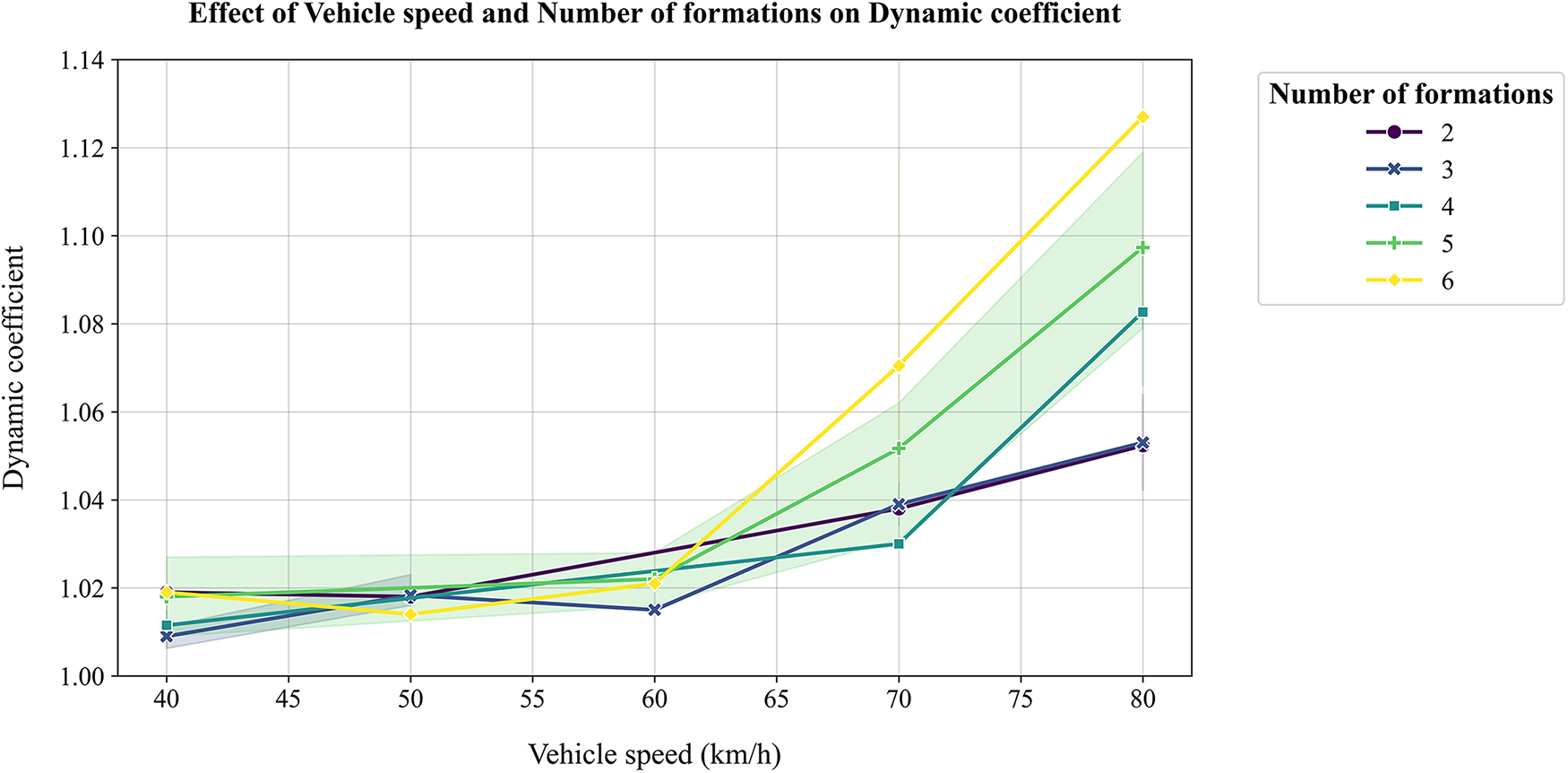
Figure 10: Interaction diagram of vehicle speed and number of formations

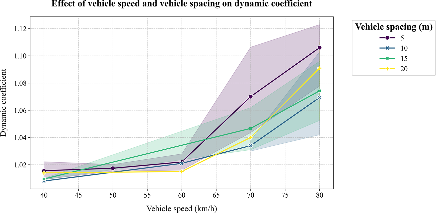
Figure 11: Interaction diagram of vehicle speed and vehicle spacing

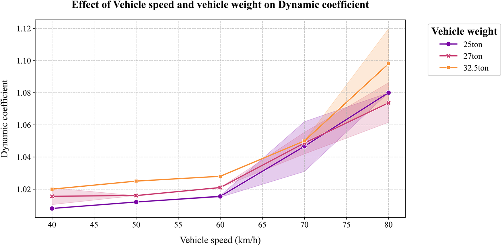
Figure 12: Interaction diagram of vehicle speed and vehicle weight

By analyzing the interaction between the speed and the number of formations, the interaction diagram shown in Fig. 10 below can be obtained.

The analysis results in Fig. 10 reveal differences in the interaction between vehicle speed and the number of formations across various speed ranges. When vehicle speed falls within the medium-speed range (50–60 km/h), the power coefficient curves for different numbers of formations show no significant overlap, indicating that the interaction between speed and the number of formations is negligible within this range. However, when vehicle speeds fall within the 40–50 km/h range or exceed 60 km/h, the power coefficients for different numbers of formations exhibit distinct linear intersections with overlapping value ranges. This indicates a significant interaction between vehicle speed and the number of formations within these speed ranges. Specifically, the dynamic coefficient for the 6-formation condition significantly increases to 1.1–1.14. Meanwhile, the dynamic coefficients for other formation conditions remain within 1.04–1.08, with their confidence intervals persistently overlapping. The results indicate that at both low and high-speed ranges, increasing the number of formations significantly exacerbates dynamic responses. A larger number of formations exerts a statistically significant adverse effect on bridge dynamic performance compared to a smaller number of formations. Differences in dynamic response patterns across speed ranges further indicate that the interaction effect between speed and the number of formations is modulated by speed level, with weaker interaction at moderate speeds. This implies that when designing and evaluating bridge structures, particular attention must be paid to the impact of vehicle traffic on bridge dynamic response within these specific speed ranges. The interaction analysis of vehicle speed and vehicle spacing can be obtained as shown in Fig. 11.

Analysis of the speed-to-spacing interaction in Fig. 11 reveals that the influence of vehicle spacing on the dynamic coefficient exhibits significant speed dependency. When speeds fall within the 40–50 km/h range or exceed 60 km/h, the dynamic coefficient curves for different vehicle spacings intersect distinctly, indicating a pronounced interaction between speed and spacing within these speed ranges. However, at 50–60 km/h, the linear intersections of the dynamic coefficients for different vehicle spacings are less pronounced. Their values range from 1.00 to 1.05, with extensive overlap in the confidence intervals, indicating that the interaction between speed and vehicle spacing is insignificant within this speed range. Notably, in the high-speed range (70–80 km/h), due to the concentrated load distribution of vehicle formations, the effects of vehicle spacing begin to diverge: the dynamic coefficient significantly increases to 1.10–1.12 at a 5-m vehicle spacing, and to 1.08–1.10 at a 20-m vehicle spacing. In contrast, the dynamic coefficient remains at 1.06–1.08 for 10-m and 15-m vehicle spacings. This indicates that both shorter and longer vehicle spacings significantly exacerbate dynamic response at high speeds.

As shown in the analysis results of the interaction between vehicle speed and vehicle weight in Fig. 12, when the speed is within the 40–70 km/h range, the power coefficient curves for different vehicle weights do not intersect. This indicates that the interaction between speed and weight is not significant within this speed range. However, when vehicle speed increases to the high-speed range of 70–80 km/h, the dynamic coefficient curves for different vehicle weights intersect distinctly. The regulatory effect of vehicle weight significantly intensifies, with the dynamic coefficient exhibiting a pronounced upward trend as vehicle weight increases. These results indicate that at higher speeds, heavier vehicle loads exert a more pronounced dynamic excitation effect on bridge structures.

To quantitatively evaluate the contributions of each influencing factor and their interactions to the bridge’s dynamic amplification factor, a general linear model is constructed based on the 44 simulation cases of platoon loading. Vehicle speed, number of formations, vehicle spacing, and vehicle weight are included as independent variables, together with all pairwise interaction terms. Analysis of variance (ANOVA) is then performed to examine the statistical significance of each effect. The results are presented in Table 6.

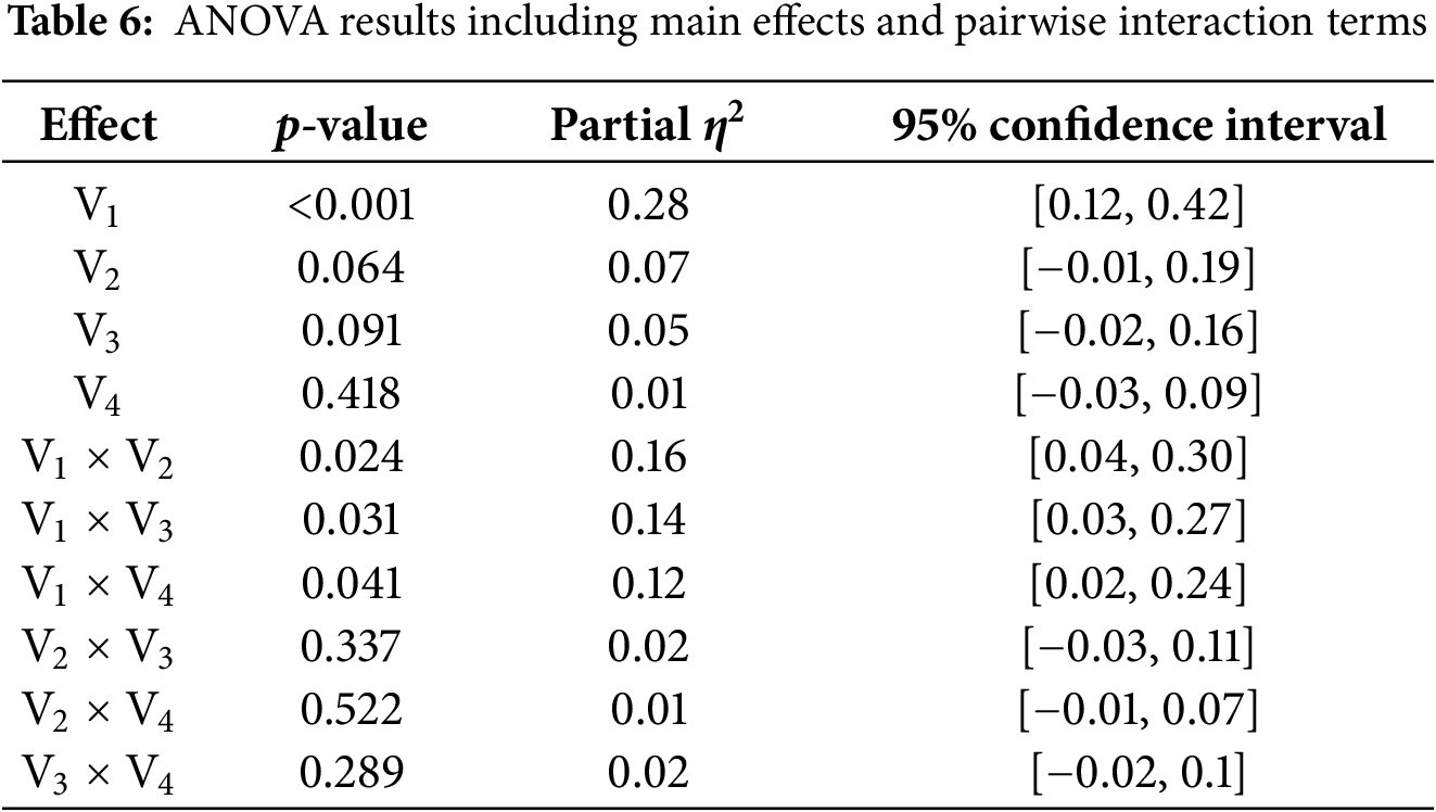
As shown in Table 6, the main effect of vehicle speed is highly significant at the 0.05 level (p-value < 0.001, partial η2 = 0.28, 95% CI [0.12, 0.42]), indicating that speed is the primary controlling factor influencing the dynamic amplification factor, with a notably large effect size. The main effects of number of formations and vehicle spacing have p-values of 0.064 and 0.091, with corresponding partial η2 values of 0.07 and 0.05. Although they do not reach significance at the 0.05 level, both exhibit a trend toward “marginal significance,” suggesting that increasing number of formations or reducing vehicle spacing tends to increase the dynamic amplification factor under the test conditions.

In contrast, the main effect of vehicle weight (p-value = 0.418, partial η2 = 0.01) is small, indicating that within the selected loading range, changes in vehicle weight alone have a relatively limited influence on the dynamic amplification factor.

Regarding interaction effects, the three interactions— “speed × number of formations,” “speed × vehicle spacing,” and “speed × vehicle weight”—are all statistically significant at the 0.05 level, with corresponding partial η2 values of approximately 0.16, 0.14, and 0.12. Their 95% confidence intervals do not include zero, indicating clear synergistic amplification effects: as vehicle speed increases, the influence of number of formations, vehicle spacing, and vehicle weight on the dynamic amplification factor becomes increasingly pronounced.

The remaining interaction terms—“number of formations × vehicle spacing,” “number of formations × vehicle weight,” and “vehicle spacing × vehicle weight”—have p-values greater than 0.05, small partial η2 values, and confidence intervals that generally span zero, suggesting that under the present experimental design and parameter ranges, these interactions are not stable and do not exhibit statistically significant effects.

Overall, the results demonstrate that vehicle speed exerts not only the strongest individual influence on the dynamic amplification factor but also significantly modulates the effects of number of formations, vehicle spacing, and vehicle weight through interaction mechanisms. This finding is consistent with the earlier correlation analysis and the qualitative patterns observed in the 3D bubble plots: under high-speed conditions, large number of formations, small vehicle spacings, and heavy loading are more likely to induce dynamic amplification effects in bridges, and thus warrant particular attention in the operational planning of autonomous truck platoons.

Analysis of the interactions between vehicle speed and the number of formations, vehicle spacing, and vehicle weight reveals that vehicle speed is the dominant factor influencing changes in the power coefficient. However, the strength and direction of its effect are significantly dependent on the synergistic effects of other variables. Specifically, at high speeds, the combined effects of a larger number of formations, shorter vehicle spacing, and heavier vehicle load cause the dynamic coefficient to surge sharply. Its 95% confidence interval completely separates from those of other variable levels, indicating statistically significant synergistic effects. Conversely, at low speeds (≤60 km/h), the distribution of dynamic coefficients across different variable levels overlaps, with confidence intervals covering each other, indicating that the interaction does not reach a significant level. Therefore, to effectively control bridge dynamic response, high-risk parameter combinations such as ‘high speed-large number of formations-small vehicle spacing-heavy load’ should be avoided under high-speed conditions. In contrast, relevant parameter restrictions can be appropriately relaxed on medium-to-low speed sections. To quantitatively reveal the specific contribution levels and directional effects of each influencing parameter on the dynamic coefficient, this paper further plots a heatmap of regression coefficients, as shown in Fig. 13 below. This visually presents the standardized regression coefficients and their significance for factors such as vehicle speed, the number of formations, vehicle spacing, and vehicle weight, thereby providing direct data support for parameter prioritization and threshold setting in the aforementioned control strategy.

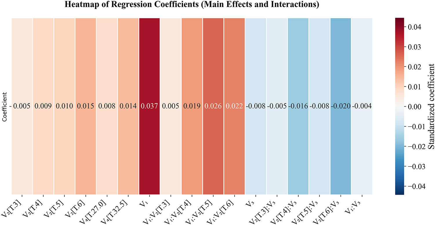
Figure 13: Regression coefficient heatmap

Analysis of the regression coefficient heatmap reveals significant variations in the influence of each variable on the bridge dynamic coefficient. To enhance descriptive efficiency, we uniformly adopt standardized variable naming corresponding to the parameter design in Table 2: V1 (vehicle speed, km/h), V2 (number of formations), V3 (vehicle spacing, m), V4 (vehicle weight, kN). The horizontal axis labels on the heatmap follow the format “V× [T. Level]”, where “V” denotes the main effect of the variable, “×” indicates an interaction term, and “[T. Level]” represents different levels of the categorical variable. For instance, V2[T.5] signifies that when the number of formations is 5, the dynamic coefficient increases by 0.01 for each standard deviation increase in the number of formations; V1:V2[T.3] indicates that when the number of formations is 3, the dynamic coefficient increases by 0.005 for each standard deviation increase in vehicle speed. The regression coefficient for vehicle speed is 0.037, indicating that each standard deviation increase in speed raises the dynamic coefficient by an average of 0.037, making it the most significant parameter among all variables. When the number of formations is 5 and vehicle speed increases, the regression coefficient for speed reaches 0.026. This indicates that under this specific formation configuration, the positive influence of speed on the dynamic coefficient surpasses that of the number of formations. In contrast, the impact of vehicle weight is relatively weak, with a coefficient below 0.01. Notably, the regression coefficient for vehicle spacing under general conditions is −0.008, suggesting that increased spacing typically helps reduce dynamic response. In summary, vehicle speed is the dominant factor influencing bridge dynamic response, with its positive effect significantly stronger than parameters such as the number of formations, vehicle spacing, and vehicle weight. It should therefore be prioritized as the key control parameter in vibration mitigation strategies for practical engineering applications. The study clearly visualizes the coupling relationship between main effects and interaction effects through heatmaps, providing a theoretical basis for optimizing vehicle formation passage strategies.

(3) The static effect of mid-span deformation

In the dense formation state, the pressure on the bridge structure increases significantly. This increased pressure may cause the stress distribution, deformation and vibration response of the bridge structure to exceed the allowable range of the design specification. By systematically analyzing the bridge responses under these special loading conditions and comparing them with code-specified loads, the deviations in structural behavior under non-standard loading scenarios can be identified. This enables a more accurate assessment of the bridge’s safety performance during actual operation and provides a basis for proposing corresponding design optimization measures and traffic management strategies.

China's bridge design specification is the General Specification for Highway Bridge and Culvert Design JTG D60-2015. The bridge design load selected in this paper is Highway-I, and the corresponding lane load is composed of uniform load and concentrated load. As demonstrated in Section 4.2 on dynamic model development, for the case studied in this paper, the standard value of uniform load is qK=10.5 kN/m. The standard value of concentrated load is PK=360 kN.

According to the load requirements of the specification, the results shown in Fig. 14 are obtained in the software.

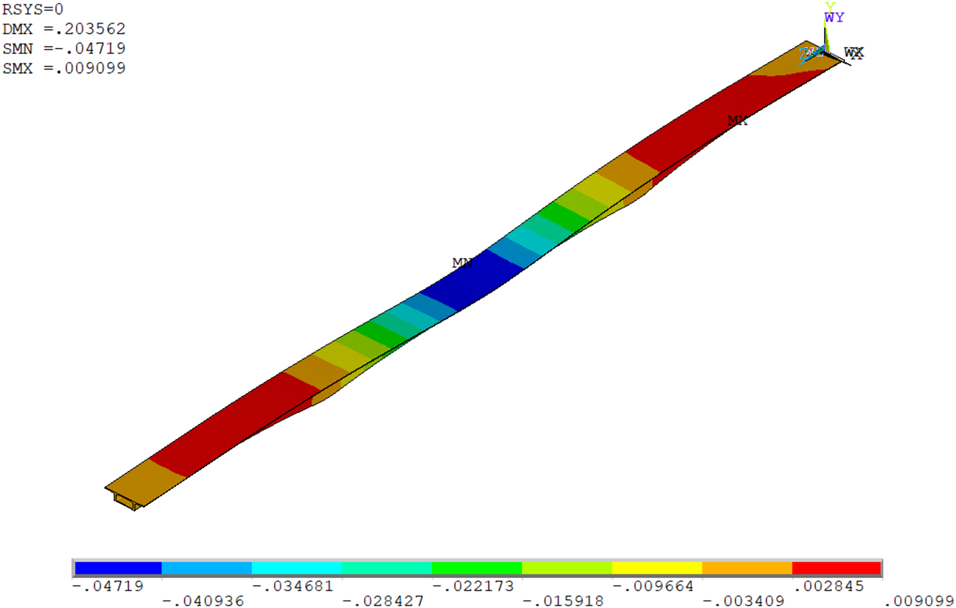
Figure 14: Specification load requirement result diagram

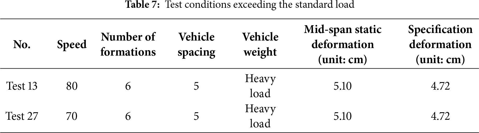
The results show that under the standard conditions, the maximum mid-span deformation displacement of the bridge is 4.72 cm, and in 44 groups of experiments, the deformation of two groups of experiments is greater than the standard requirements, as shown in Table 7. The indexes of the two groups of experiments are: test 13 with speed of 80 km/h, formation number of 6, vehicle spacing of 5 m, vehicle weight of 32.5 kN and test 27 with speed of 70 km/h, formation number of 6, vehicle spacing of 5 m, vehicle weight of 32.5 kN. These two sets of experimental conditions show that when the number of truck formations increases, the weight of the vehicle monomer increases, and the vehicle spacing is further reduced, the mid-span deformation of the bridge increases, and it has exceeded the specification requirements under these two sets of experimental conditions.

Therefore, in order to ensure the stability and safety of the bridge structure, the size of the formation, vehicle speed, vehicle spacing and cargo capacity must be strictly controlled. Specifically, when the truck formation passes through the engineering background bridge, when the vehicle spacing is 5 m and the vehicle weight is 32.5 kN, it is recommended that the number of formation vehicles should not exceed 5 to effectively reduce the dynamic impact of the formation on the bridge structure. In addition, in order to reduce the dynamic effect of the formation on the bridge, it is recommended that the vehicle speed should be controlled below 60 km/h. Finally, the vehicle load must be strictly controlled within the standard range, and overweight and overload behavior must be prohibited to ensure the normal operation and long-term durability of the bridge.

5  Discussion

Based on a vehicle–bridge coupled dynamic model and a mixed-level orthogonal experimental design, this study systematically investigates the dynamic response characteristics of autonomous truck platoon loading. The multi-factor interaction analysis demonstrates that vehicle speed exerts a significant moderating effect on the influences of number of formations, vehicle spacing, and vehicle weight. In particular, under high-speed conditions (≥70 km/h), a synergistic amplification effect emerges among large number of formations, short vehicle spacings, and heavy loading, resulting in dynamic amplification factors notably higher than those of other factor combinations. In contrast, under medium–low speeds, the interaction effects among these factors diminish considerably, the distributions of dynamic amplification factors become largely overlapping, and the structural responses are more stable. By incorporating code-based deflection checks, the study further identifies two critical loading scenarios—characterized by high speed, a six-vehicle platoon, a 5 m spacing, and heavy loading—that result in mid-span deflections exceeding the design live-load limit. This finding underscores that the combination of high speed, large platoon size, short vehicle spacing, and heavy loading represents a typical high-risk operational condition for autonomous truck platoons, necessitating heightened attention in traffic management and potential updates to design specifications.

In addition, for computational efficiency, this study assumes an ideally smooth bridge deck. While this simplification helps isolate the independent effects of platoon parameters, it neglects the excitation induced by road surface roughness. As a result, the actual dynamic amplification factors in real-world operations may be higher than the numerical results predicted herein. Future research should incorporate road roughness spectra of various grades and extend the analysis to a broader range of bridge types and vehicle models with more complex degrees of freedom, in order to comprehensively evaluate the dynamic safety performance of bridges under adverse operating conditions.

6  Conclusion

Based on a vehicle–bridge coupled dynamic model and a mixed-level orthogonal experimental design, this study systematically investigates the effects of vehicle speed, number of formations, vehicle spacing, vehicle weight, and their interactions on the dynamic amplification factor and mid-span deflection of a large-span continuous beam bridge. The main conclusions are as follows:

(1) Vehicle operating speed is the dominant factor influencing the dynamic amplification factor of the bridge. Analysis of the main effects shows that significant interactions exist between speed and number of formations, between speed and vehicle spacing, and between speed and vehicle weight. Notably, when the vehicle speed exceeds 60 km/h, the DAF increases markedly.

(2) Large number of formations, short vehicle spacings, and heavy vehicle loading can jointly lead to substantial increases in mid-span deformation, potentially exceeding the values specified by design codes. This highlights the necessity of strictly controlling number of formations, inter-vehicle spacing, and vehicle weight to ensure structural stability and operational safety of the bridge.

(3) To maintain structural stability and ensure safe platoon operation for the bridge investigated in this study, the following operational recommendations are proposed: vehicle speed should be limited to below 60 km/h, vehicle spacing should be maintained within 10–15 m, and number of formations should be restricted to no more than five vehicles.

(4) This study is based on a single span configuration, a limited range of platoon parameters, and a simplified vehicle model, without incorporating different levels of road surface roughness. Future work should extend the analysis to a broader variety of bridge types, surface roughness grades, and platoon configurations to improve the generalizability of the findings.

Acknowledgement: The authors would like to thank the support by “111” Project “Centre on Safety and Intelligent Operation of Sea Bridge (D21013)”.

Funding Statement: The authors received no specific funding for this study.

Author Contributions: Conceptualization, Zhihua Xiong, Xiaoling Liu, Yinfeng Wang; methodology, Zhihua Xiong, Xiaoling Liu; validation, Zhihua Xiong; investigation, Xiaoling Liu, Yinfeng Wang; data curation, Zhihua Xiong; writing—original draft preparation, Zhihua Xiong, Xiaoling Liu, Yinfeng Wang; writing—review and editing, Xiaoling Liu; supervision, Zhihua Xiong, Xiaoling Liu, Yinfeng Wang. All authors reviewed the results and approved the final version of the manuscript.

Availability of Data and Materials: The data that support the findings of this study are available from the Corresponding Author, Xiaoling Liu, upon reasonable request.

Ethics Approval: Not applicable.

Conflicts of Interest: The authors declare no conflicts of interest to report regarding the present study.

References

1. Yan J, Deng L, He X. Optimal transverse position for overweight trucks to cross simply supported multi-girder bridges. Adv Struct Eng. 2018;21(9):1251–61. doi:10.1177/1369433217737116. [Google Scholar] [CrossRef]

2. Liu M, Sun Q, Yu H, Yang J, Zhang T. Static and dynamic test analysis of a 12-years old 14 000-ton cable-stayed bridge used swivel construction technology. Arch Civ Eng. 2021;67(4):369–81. doi:10.24425/ace.2021.138505. [Google Scholar] [CrossRef]

3. Li C, Lu B, Wang C, Peng W. Dynamic performance assessment of a novel hybrid bridge system with spread steel box girders. J Bridge Eng. 2022;27(1):04021097. doi:10.1061/(asce)be.1943-5592.0001805. [Google Scholar] [CrossRef]

4. Lu X, Kim CW, Chang KC. Finite element analysis framework for dynamic vehicle-bridge interaction system based on ABAQUS. Int J Str Stab Dyn. 2020;20(3):2050034. doi:10.1142/s0219455420500340. [Google Scholar] [CrossRef]

5. Zhao Y, Guo X, Su B, Sun Y, Zhu Y. Multi-lane traffic load clustering model for long-span bridge based on parameter correlation. Mathematics. 2023;11(2):274. doi:10.3390/math11020274. [Google Scholar] [CrossRef]

6. Tan Y, He X, Shi L, Zheng S, Zhang Z, Wang X. Reinforcement effect evaluation on dynamic characteristics of an arch bridge based on vehicle-bridge coupled vibration analysis. Comput Model Eng Sci. 2022;131(2):1041–61. doi:10.32604/cmes.2022.018543. [Google Scholar] [CrossRef]

7. Ling T, Deng L, He W, Cao R, Zhong W. Determination of dynamic amplification factors for small- and medium-span highway bridges considering the effect of automated truck platooning loads. Mech Syst Signal Process. 2023;204(1):110812. doi:10.1016/j.ymssp.2023.110812. [Google Scholar] [CrossRef]

8. Song Y, Hu B, Meng X. Efficient dynamic performance prediction of railway bridges situated on small-radius reverse curves. Shock Vib. 2024;2024(1):6666054. doi:10.1155/2024/6666054. [Google Scholar] [CrossRef]

9. Li Y, Qin L, Li Z, Yang T. Dynamic performance of strengthened concrete-filled steel tubular arch bridge due to moving vehicles. J Aerosp Eng. 2019;32(1):04018113. doi:10.1061/(asce)as.1943-5525.0000934. [Google Scholar] [CrossRef]

10. Kaloop MR, Kim KH, Elbeltagi E, Jin X, Hu JW. Service-life evaluation of existing bridges subjected to static and moving trucks using structural health monitoring system: case study. KSCE J Civ Eng. 2020;24(5):1593–606. doi:10.1007/s12205-020-2128-1. [Google Scholar] [CrossRef]

11. Yang YB, Xu H, Zhang B, Xiong F, Wang ZL. Measuring bridge frequencies by a test vehicle in non-moving and moving states. Eng Struct. 2020;203(ST10):109859. doi:10.1016/j.engstruct.2019.109859. [Google Scholar] [CrossRef]

12. OBrien EJ, Brownjohn JMW, Hester D, Huseynov F, Casero M. Identifying damage on a bridge using rotation-based Bridge Weigh-In-Motion. J Civ Struct Health Monit. 2021;11(1):175–88. doi:10.1007/s13349-020-00445-w. [Google Scholar] [CrossRef]

13. Mo S, Chen K, Huang Z, Zhang W. Dynamic analysis and optimization of vehicle-bridge interaction system under road roughness and time variability of element interpolation function. Transp Res Rec J Transp Res Board. 2024;2678(8):294–309. doi:10.1177/03611981231215336. [Google Scholar] [CrossRef]

14. Zhang Y, Li W, Ji Z, Wang G. Vehicle ride comfort analysis based on vehicle-bridge coupled vibration. Shock Vib. 2021;2021(1):5285494. doi:10.1155/2021/5285494. [Google Scholar] [CrossRef]

15. Xiao X, Sun Z, Shen W. A Kalman filter algorithm for identifying track irregularities of railway bridges using vehicle dynamic responses. Mech Syst Signal Process. 2020;138(7–8):106582. doi:10.1016/j.ymssp.2019.106582. [Google Scholar] [CrossRef]

16. Moghimi H, Ronagh HR. Impact factors for a composite steel bridge using non-linear dynamic simulation. Int J Impact Eng. 2008;35(11):1228–43. doi:10.1016/j.ijimpeng.2007.07.003. [Google Scholar] [CrossRef]

17. Deng L, He W, Shao Y. Dynamic impact factors for shear and bending moment of simply supported and continuous concrete girder bridges. J Bridge Eng. 2015;20(11):04015005. doi:10.1061/(asce)be.1943-5592.0000744. [Google Scholar] [CrossRef]

18. Zhang Y, Cai CS, Shi X, Wang C. Vehicle-induced dynamic performance of FRP vs. concrete slab bridge. J Bridge Eng. 2006;11(4):410–9. doi:10.1061/(asce)1084-0702(2006)11:4(410). [Google Scholar] [CrossRef]

19. Ma L, Li Z, Xu H, Cai CS. Numerical study on the dynamic amplification factors of highway continuous beam bridges under the action of vehicle fleets. Eng Struct. 2024;304(12):117638. doi:10.1016/j.engstruct.2024.117638. [Google Scholar] [CrossRef]

20. Thulaseedharan NP, Yarnold MT. Prioritization of Texas prestressed concrete bridges for future truck platoon loading. Bridge Struct. 2021;16(4):155–67. doi:10.3233/brs-210181. [Google Scholar] [CrossRef]

21. Tohme R, Yarnold M. Steel bridge load rating impacts owing to autonomous truck platoons. Transp Res Rec J Transp Res Board. 2020;2674(2):57–67. doi:10.1177/0361198120902435. [Google Scholar] [CrossRef]

22. Ling T, Cao R, Deng L, He W, Wu X, Zhong W. Dynamic impact of automated truck platooning on highway bridges. Eng Struct. 2022;262(1):114326. doi:10.1016/j.engstruct.2022.114326. [Google Scholar] [CrossRef]

23. AASHTO. LRFD bridge design specifications. 8th ed. Washington, DC, USA: American Association of State Highway and Transportation Officials; 2017. [Google Scholar]

24. Liu X, Zhang X, Wang Y. A rapid detection method for bridges based on impact coefficient of standard bumping. Math Probl Eng. 2018;2018(2):9195289. doi:10.1155/2018/9195289. [Google Scholar] [CrossRef]

25. GB 1589-2016. Limits of dimensions, axle load and masses for motor vehicles, trailers and combination vehicles. Beijing, China: SAC; 2016. (In Chinese). [Google Scholar]

26. JTG 3362-2018. Specifications for design of highway reinforced concrete and prestressed concrete bridges and culverts. Beijing, China: China Communications Press; 2018. (In Chinese). [Google Scholar]

27. JTG D60-2015. General specifications for design of highway bridges and culverts. Beijing, China: China Communications Press; 2015. (In Chinese). [Google Scholar]

28. Hu W, Ou Z, Peng Q. Mixed-level designs with orthogonality and relatively optimal Run order. J Appl Stat. 2024;51(13):2493–511. doi:10.1080/02664763.2023.2301323. [Google Scholar] [PubMed] [CrossRef]

29. Zhang Y, Zhu J. Damage identification for bridge structures based on correlation of the bridge dynamic responses under vehicle load. Structures. 2021;33:68–76. doi:10.1016/j.istruc.2021.04.022. [Google Scholar] [CrossRef]

30. He H, Yang C. Automated truck platooning-bridge interaction: assessing dynamic impacts on drilled shaft foundations. J Bridge Eng. 2025;30(5):04025015. doi:10.1061/jbenf2.beeng-7052. [Google Scholar] [CrossRef]