An Efficient Differential Evolution for Truss Sizing Optimization Using AdaBoost Classifier

1  Introduction

Nowadays, global competition has posed a big challenge for industrial companies to offer quality products at lower prices. The situation is similar for the field of construction where the contractors are frequently pressured to reduce costs while maintaining high standards. In this case, optimizing the weight of structures is seen as an effective strategy to gain a competitive advantage. Traditionally, the structure is often designed manually following the “trial-and-error” method. The final structural solution received from this way is deeply influenced by the designers’ experience and intuition. Therefore, in order to help the designers find the best solution, the optimization algorithms were applied to the design process and have been constantly developed.

Generally, optimization algorithms are categorized into two groups: gradient-based group and metaheuristic group. The gradient-based optimization finds the minimum by going in the direction opposite sign of the derivative of the function. Hence, the speed of convergence is seriously influenced by the starting point, and the gradient-based optimization may fall to the local minimum. Additionally, the function is sometimes difficult or impossible to calculate the derivative. Contrary to gradient-based methods, metaheuristics do not require the calculation of derivative value. Instead, these algorithms use the randomization principle to find the optimum. By searching for a large set of solutions spreading over the design space, metaheuristics can easily escape a local optimum and eventually reach a global optimum. Because of their advantages like easy implementation as well as robustness, metaheuristics are increasingly applied to civil engineering problems. Some outstanding algorithms that are widely used in structural optimization can be listed here such as Genetic Algorithm (GA) [1,2], Evolution Strategies (ES) [3,4], Differential Evolution (DE) [5,6], Particle Swarm Optimization (PSO) [7,8]. Some recently proposed algorithms have shown competitive performance, for example, Artificial Bee Colony (ABC) [9], Harmony Search (HS) [10,11], Teaching-Learning-Based Optimization (TLBO) [12,13], Colliding Bodies Optimization (CBO) [14,15].

Despite many advantages, metaheuristics have one common drawback of requiring a large number of fitness evaluations. It should be highlighted that for structural optimization problems, the objective function can be quickly determined but the computation of constraints is very costly due to involving the structural analysis. Conducting a high number of structural analyses is the most time-consuming task when optimizing structures. Therefore, reducing the number of structural analyses becomes an important goal. To overcome this challenge, many efforts have been made to improve the performance of existing algorithms [16–19]. Besides, using surrogate models instead of computationally expensive structural analyses is a potential solution [20–28]. In recent decades, due to the fast growth of Artificial Intelligence (AI), especially Machine Learning (ML), the topic regarding ML-based surrogate-assisted metaheuristic algorithms has attracted interest from researchers.

Based on the literature, there are several strategies for managing surrogate models. The most straightforward way is to build surrogate models based on the data obtained from the original fitness evaluations and the whole models will be used during the optimization process. Since 1997, Papadrakakis et al. [20] employed feed-forward neural networks (NNs) to predict the response of structures. These NNs were combined with the ES algorithm for optimizing shapes and sections of structures. To cope with the error of NNs, a correction technique was proposed, in which the allowable constraint values were adjusted proportionally to the maximum error for the testing dataset. The research was then extended to large-scale 3D roof trusses [21]. Similarly, structural analyses were replaced by NNs during the GA-based optimization process [22]. In more detail, three kinds of NN including radial basis function (RBF) network, generalized regression (GR) network, and counter-propagation (CP) network were used for optimizing 25-bar truss structure as well as 1300-bar dome structure. The obtained results showed that the RBF networks outperformed the other two networks. In 2019, Taheri et al. [23] combined the RBF neural networks and the ABC algorithm for solving the size, shape, and topology optimization problems of steel lattice towers. Next, the adaptive fuzzy neural inference system (ANFIS) network is used instead of structural analyses carried out by MSTOWER software when optimizing transmission towers [24]. Nguyen et al. [25] utilized two deep NNs separately to estimate the stresses and displacements when optimizing truss structures. Recently, Mai et al. [26] also used deep NNs to reduce the computation cost of the design optimization of geometrically nonlinear trusses. This strategy has been proven to be time-effective but the designs were not the true optimal designs due to the inaccuracy of surrogate models.

To avoid falling a false optimum, both the exact functions and the approximate functions are used simultaneously. For example, in [27], the combination of NN and GA was adapted to optimize transmission towers based on this strategy. The optimization process employed in this study comprises two stages: in the first stage, the RBF networks were used as structural analyzers until the stopping criterion and in the second stage, the exact structural analyses were conducted. Chen et al. [28] proposed a hybrid approach, in which the near-optimal point was located by the ES algorithm with the help of NN-based surrogate models, and the sequential quadratic programming algorithm was then used to find the exact optimal point.

These existing studies have been used a similar approach, in which the surrogate models have been constructed by regression techniques with the aim of predicting the degree of constraint violation of candidates. While this approach is very intuitive and has been successfully applied in a lot of studies, this is not the only one. An alternative approach is to use the classification technique to build surrogate models. In the literature, the classification-based surrogate models have been successfully applied to solve optimization problems. For instance, Kramer et al. [29] used a classification model for predicting the feasibility of the solutions. However, a feasible solution can be classified as an infeasible solution due to the poor quality model, leading to the rejection of potential solutions. Therefore, the constraint boundary is shifted to the infeasible region by a small distance to limit this error. Another study [30] proposed a probability which is called the influence coefficient to prevent the misclassification of the surrogate model. In 2018, Wang et al. [31] introduced a technique in which the boundary is adjusted to decrease the possibility of classifying feasible solutions to be infeasible.

Although classification techniques have been used previously, the proposed method in the present work is different. Instead of using an additional parameter as in former works, this study employs a classification surrogate model in conjunction with the direct comparison of the objective function values. In detail, a classifier will be built to identify whether the structural solution satisfies the design constraints or not. When optimizing the weight of trusses, if a new solution is predicted to violate the design constraints and its weight is heavier than that of the parent solution, it will be discarded without conducting structural analysis. In this way, some unnecessary structural analyses will be reduced and consequently, the computational time will be shortened.

The classification technique used in this study is Adaptive Boosting (as known as AdaBoost) developed by Freund et al. [32]. The AdaBoost classifier is combined with the DE algorithm to form an efficient optimizer called CaDE. AdaBoost is selected because it has been proven as a powerful algorithm for the task of classifying the structural safety of trusses [33]. In addition, the choice of the DE algorithm is motivated by its simplicity and robustness. The proposed method CaDE is first examined for the weight optimization of truss structures.

The remainder of this paper is arranged as follows. A brief introduction of the DE algorithm and the AdaBoost classifier are given in Section 2. The truss sizing optimization is presented in Section 3.1. Next, the detail of the proposed method CaDE is described in Section 3.2. Computational experiments are conducted in Section 4, in which, six benchmark trusses are optimized according to the proposed method to show its efficiency. In addition, a real-size transmission tower is also designed using the proposed method to exhibit its applicability in practice. Finally, Section 5 concludes this paper.

2  Background Information

2.1 Differential Evolution Algorithm

Differential Evolution is a metaheuristic algorithm that was firstly introduced by Storn et al. [34] in 1995. Thanks to its simplicity, this algorithm is widely applied to many fields such as communication, transportation, aerospace, civil engineering, etc. Since the first introduction, DE has been taken a top rank in many competitions relating to evolutionary computation [35,36]. Particularly, some studies that compare the performance of metaheuristic algorithms in structural optimization have been conducted [37]. The results show that DE outperforms the remaining algorithms.

DE is designed based on the natural evolutionary mechanism. According to the Darwinian theory, the main driving forces of evolution are mutation and natural selection. Similarly, DE consists of four basic steps as shown in Fig. 1, in which the initialization step is conducted one time at the first of the optimization process while three remaining steps are repeated till a stopping criterion is satisfied.

Figure 1: Main steps of differential evolution

The optimization process begins with an initialization of a population pop0 containing NP individuals. Each individual representing a candidate of the optimization problem is a D-dimensional vector:

xi(0)={xi,1(0),xi,2(0),…,xi,D(0)}(1)

In order to find the global optimum, the initial population should be spread over the search space as much as possible. The most widely used method for generating the initial population is to use the uniform distribution. In detail, the jth component of the ith vector can be initialized based on this formula:

xi,j(0)=xjmin+randi,j[0,1](xjmax−xjmin)(2)

where: xjmin and xjmax are the lower and upper bounds for the jth component of the ith vector; rand [0, 1] is a uniformly distributed random number in the range [0, 1].

Secondly, DE creates NP mutant vectors vi(t) corresponding to NP target vector xi(t) via the mutation operator. The classical mutation operator is to add a scaled difference vector between two random vectors to the third vector. It can be written in the mathematical form as follows:

vi(t)=xr1(t)+F×(xr2(t)−xr3(t))(3)

where: r1 ≠ r2 ≠ r3 ≠ i are three integers that are randomly chosen from the range [1, NP]; t is the current generation number; F is the scaling factor.

The above mutation strategy is called “DE/rand/1” where the term “rand” means random and the number “1” denotes that only one difference vector is added. Besides “DE/rand/1”, four mutation strategies that were proposed by Storn et al. [34] are listed below:

``DE/best/1''vi(t)=xbest(t)+F×(xr1(t)−xr2(t))(4)

``DE/target - to - best/1''vi(t)=xi(t)+F×(xbest(t)−xi(t))+F×(xr1(t)−xr2(t))(5)

``DE/rand/2''vi(t)=xr1(t)+F×(xr2(t)−xr3(t))+F×(xr4(t)−xr5(t))(6)

``DE/best/2''vi(t)=xbest(t)+F×(xr1(t)−xr2(t))+F×(xr3(t)−xr4(t))(7)

in which: xbest(t) is the best individual of the current population.

In the crossover step, a trial vector ui(t) is constructed by taking some components from xi(t) and the rest from vi(t). It can be expressed as:

ui,j(t)={vi,j(t)if j=K or randi,j[0,1]≤Crxi,j(t)otherwise(8)

where: ui,j(t), vi,j(t) and xi,j(t) are the jth component of ui(t), vi(t), and xi(t), respectively; K is a random integer in [1,D] to ensure that ui(t) differs xi(t) by getting at least one component from vi(t); and Cr is called the crossover rate.

Based on natural selection, only the fittest survive. For minimization problems, the fitness is measured through the value of the objective function. Only the one having the lower value of the objective function will be kept for the next generation. It can be described as follows:

xi(t+1)={ui(t)if f(ui(t))≤f(xi(t))xi(t)otherwise(9)

where: f(.) is the objective function that needs to be optimized.

2.2 AdaBoost Classifier

There exist many powerful machine learning classification models such as Support Vector Machine or Neural Networks. The abovementioned algorithms are categorized into the single learning group. However, there exists another group of algorithms, called ensemble methods, in which several classifiers are combined with the aim of improving the accuracy. Ensemble methods have been proven to be very effective for classification tasks. In this study, a boosting method, called AdaBoost, is employed. The idea of this algorithm is to train iteratively several weak learners using the weighted training data, and then incorporate them into the final classifier [32]. The weak learners can be any single learning algorithm, however, the most commonly used one is the Decision Tree. In the following section, the background theory of the AdaBoost classifier is presented.

Generally, AdaBoost produces several classifiers, called weak classifiers, each of them has a proper weight based on its accuracy. The final prediction is the combination of the output of weak classifiers using the weight majority voting technique. The more accurate classifier will contribute more impact on the final prediction by assigning a higher weight. In addition, AdaBoost keeps a set of weights over the training data. Initially, the weights of all samples are set equally. After an iteration, the weights of samples that were misclassified by the previous weak classifier are increased. It ensures that those samples will receive the attention of the weak classifier on the next iteration. The AdaBoost algorithm is illustrated in Fig. 2.

Figure 2: Illustration of the AdaBoost algorithm

Suppose the training dataset is DB = {(x1, y1), (x2, y2), …, (xn, yn)} in which xi, i = 1, 2, …, n is a p-dimensional input vector containing p features; yi ∈{+1, −1} is the output; and n is the number of samples in the training dataset.

AdaBoost begins by initializing sample weights uniformly as:

w1={w1,1,w1,2,…,w1,n};w1,i=1n;i=1,2,…,n(10)

where: w1,i is the initial weight of the sample (xi, yi).

Then a process of four basic steps is iteratively conducted for T times. On iteration t, the weak classifier is ht, and the weight vector is wt = {wt,1, wt,2, …, wt,n}.

Step 1: the classifier ht is fit to the weighted training data:

ht(x)=DecisionTree(DB,wt)(11)

where: DecisionTree(.) indicates a single tree classifier.

Step 2: the error of the classifier on this iteration is calculated as follows:

et=∑i=1nwt,i1(ht(xi)≠yi)(12)

where: 1(ht(xi) ≠ yi) is the function that returns 1 for correctly classified samples while 0 for misclassified samples.

Step 3: The weight of the weak classifier ht can be determined based on its accuracy as follows:

αt=12ln⁡(1−etet)(13)

Step 4: the weights of samples are updated according to the following rule:

w(t+1),i=wt,iexp⁡(−αtyiht(x))∑i=1nw(t+1),i(14)

After T such iterations, T weak classifiers ht, t = 1, 2,…, T are obtained. The final output is the weighted sum of the outputs of these weak classifiers:

H(x)=sign{∑t=1Tαtht(x)}(15)

where: sign(x) is a function that returns −1 if x < 0, + 1 if x > 0, 0 if x = 0.

3  The Proposed Method CaDE

3.1 Truss Sizing Optimization Using DE

Optimizing a truss structure is a specific constrained optimization problem where the objective function is frequently the weight of the truss structure and the constraints relate to the structural behavior like stress, displacement, or vibration conditions. Three categories of truss optimization problems include size, shape, and topology optimization, in which size optimization is widely used in practical design. For size optimization, the member cross-sectional areas are considered as design variables. The mathematical formulation of this type of optimization problem is expressed as follows:

Find A={ A1,A2,…,Ang }to minimize W(A)=ρ∑i=1ngAi∑j=1nm(i)Ljsubject to:{ gk(A)≤0,k=1,2,…,ncAi,min≤Ai≤Ai,max,i=1,2,…,ng(16)

where: A is a vector containing ng design variables; W(A) is the objective function which is the weight of the whole truss structure in this case; ρ is the density; Ai denotes a design variable which is the cross-sectional area of members belong to the ith group; Lj is the length of the jth member; ng is the number of groups; nm(i) is the number of members belong to the ith group; gk(A) is the kth constraint; nc is the number of constraints; Ai,min and Ai,max are the lower and upper bounds of the design variable Ai, respectively.

To apply metaheuristic algorithms which are originally designed for unconstrained optimization, the most widely-used technique is to use the fitness function instead of the objective function:

Fit(A)={W(A)+P(A)ifcv(A)>0W(A)otherwise(17)

in which: Fit(A) is the fitness function; and P(A) is the penalty function which is added whenever any constraint is violated; cv(A) is the degree of constraint violation that is defined as the sum of all constraint violations:

cv(A)=∑maxk⁡(0,gk(A))(18)

3.2 Accelerating DE with AdaBoost Classifier

The objective function of structural optimization problems, for example, the weight of structures, can be easily calculated by multiplying the volume of all members with their material density. However, the determination of the fitness function is very costly due to conducting a computationally expensive structural analysis. As result, the computation time of metaheuristic optimization tasks that require thousands or even millions of fitness function evaluations becomes prohibitively high.

Surrogate models have been frequently constructed to simulate the response of structures, and they have been used to quickly evaluate the fitness of individuals instead of exact structural analyses. Although the accuracy of surrogate modeling techniques has been greatly improved in recent years, there is always an error between the predictions and the ground truth due to the complexity of the structural response as well as the limitation of training data. Therefore, the direct replacement of exact structural analysis with surrogate models may lead to a false optimum [20–25].

The proposed method employs surrogate models in a different manner. The idea behind the proposed method is based on an observation that a trial vector that violates any constraint and has a larger objective function value is largely worse than its target vector and it cannot survive the selection. Detecting and eliminating these worse trial vectors during the optimizing process can save many useless structural analyses. The objective function of structural optimization problems can be quickly determined but the constraint verification is very costly due to performing a structural analysis. It leads to the idea of constructing a surrogate model that can quickly evaluate the safety state of the structure. Using regression models to estimate the degree of constraint violation for this task is not necessary. Instead, a classification model that can distinguish whether or not the individual satisfies constraints is sufficient.

The concept of the proposed method is the application of a machine learning classifier to identify trial vectors that are most likely worse than these target vectors during the optimization process. In this work, the AdaBoost algorithm is employed for that purpose and the proposed method is called CaDE. The pseudo-code of the CaDE is described in Algorithm 1.

Note: where: g is the current iteration number; DB is the database for training model; NP is the size of the population; F is the scaling factor; Cr is the crossover rate; n_iter1 is the numbers of iterations for the model building phase; max_iter is the number of iterations of the whole optimization process; Mutation, Crossover, and Selection are three basic operators of the DE as described in Section 2.1; C(.) is the AdaBoost classifier; W(.) is the objective function.

Generally, the CaDE has two phases: the model building phase and the model employing phase. The CaDE algorithm begins by initializing a population of NP vectors pop0 = {xi(0) | i = 1, 2, …, NP}. It is noted that the initial population is generated using the Latin Hypercube Sampling (LHS) technique because of its good space-filling capability. Each vector xi(0) is checked design constraints, and the label yi(0) is assigned using the following formula:

yi={−1ifcv(xi)>0+1otherwise(19)

As a result, the initial dataset DB consists of NP data samples {(xi(0), yi(0)) | i = 1, 2, …, NP}. Next, three operators (Mutation, Crossover, and Selection) are carried out sequentially as the original DE algorithm. All trial vectors ui(g) produced by the Mutation and Crossover operators are checked design constraints and assigned a label yi(g) according to Eq. (19). All obtained results (ui(g), yi(g)) are also saved into the database DB. The loop is terminated after (n_iter1−1) iterations. The final dataset comprises n_iter1 × NP data samples. At the end of this phase, an AdaBoost classification C model has been trained by the dataset DB as presented in Section 2.2.

In the model employing phase, each trial vector ui(g) is preliminarily evaluated using the classification model C. At this time, two conditions are applied in determining which trial vectors to go to the selection step or not. In more detail, a trial vector is rejected without exact evaluation when it has two conditions simultaneously: (i) it is predicted to violate design constraints (ypred_i(g) = −1), and (ii) its objective function value is larger than that of the corresponding target vector (W(ui(g)) > W(xi(g))). Otherwise, the constraint violation of the trial vector is evaluated using the structural analysis and the Selection operator is then conducted as usual. The model employing phase lasts until the pre-defined number of iteration max_iter reaches.

4  Numerical Experiments

Numerical experiments are performed on a personal computer with CPU Intel Core i5 2.5 GHz, 8 Gb RAM, and Windows 10 64 bit OS. The DE algorithm and the CaDE algorithm are developed by the authors using the Python programming language, meanwhile, the AdaBoost classifier is built using the open-source library scikit-learn [38]. The Python in-house codes for finite element analysis of truss structures are developed based on the direct stiffness method described in [39].

4.1 Illustrative Example

A three-bar truss example is carried out to illustrate the application of the CaDE algorithm to structural optimization. Although this structure is simple and the constraints can be directly evaluated, the stresses of the members are still determined through the finite element analyses in this experiment. This problem is used as an illustrative example because it has only two variables and it can be easily visualized.

The geometry, loading, and boundary conditions of the structure are presented in Fig. 3. The objective of this example is to find the cross-sectional areas A1 and A2 to minimize the weight of the truss while satisfying the condition that the stresses in all bars do not exceed the allowable stress. This problem is stated as follows:

Find    x=A={ 0.1≤A1,A2≤1 }to minimize W(A)=(22A1+A2)Lsubject to  gk(A)=σk−[ σ ]≤0,k=1,2,3(20)

in which: the applied force P = 2 kN; L = 100 cm; σk is the stress in the kth member; and the allowable stress [σ]=2 kN/cm2.

Figure 3: Three-bar truss structure

As mentioned above, the objective function W(A) should be transformed into the fitness function. In this example, the fitness function is defined as Fit(A) = W(A)(1 + cv(A)) and it is plotted in Fig. 4.

Figure 4: Visualization of the fitness function of the three-bar truss structure

The DE algorithm starts by initializing an initial population pop0 of NP individuals. In this example, the number of individuals of a population is set to NP = 20. The initial individuals are represented together with the 2-D contour plot of the fitness function as shown in Fig. 5a. Then, three operators including mutation, crossover, and selection are sequentially performed to produce a population pop1 for the next iteration with two optimization parameters as follows: F  =  0.8, Cr  =  0.9. The manner in which the mutant vector vi(0) and the trial vector ui(0) are produced from the target vector xi(0) is shown in Fig. 5b. If the fitness function value of the trial vector ui(0) is smaller than that of the target vector xi(0), the trial vector ui(0) is selected to be the target vector xi(1) of the next population. Otherwise, the trial vector ui(0) is discarded and the target vector xi(0) is kept for the next iteration.

Figure 5: Visualization of three first operators of the DE algorithm

The above process is repeated until the stopping condition is reached. In this example, the stopping condition is set to be after 100 iterations. The populations at several iterations are shown in Fig. 6. It can be seen that all individuals of the population tend to move closer to the global optimal position during the optimization process. At the final iteration, almost all individuals are concentrated at the global optimal position. The optimal design found by the DE algorithm is as follows: A1 = 0.789 cm2 and A2 = 0.408 cm2. The number of structural analyses that must be conducted is nSA = 2000 times.

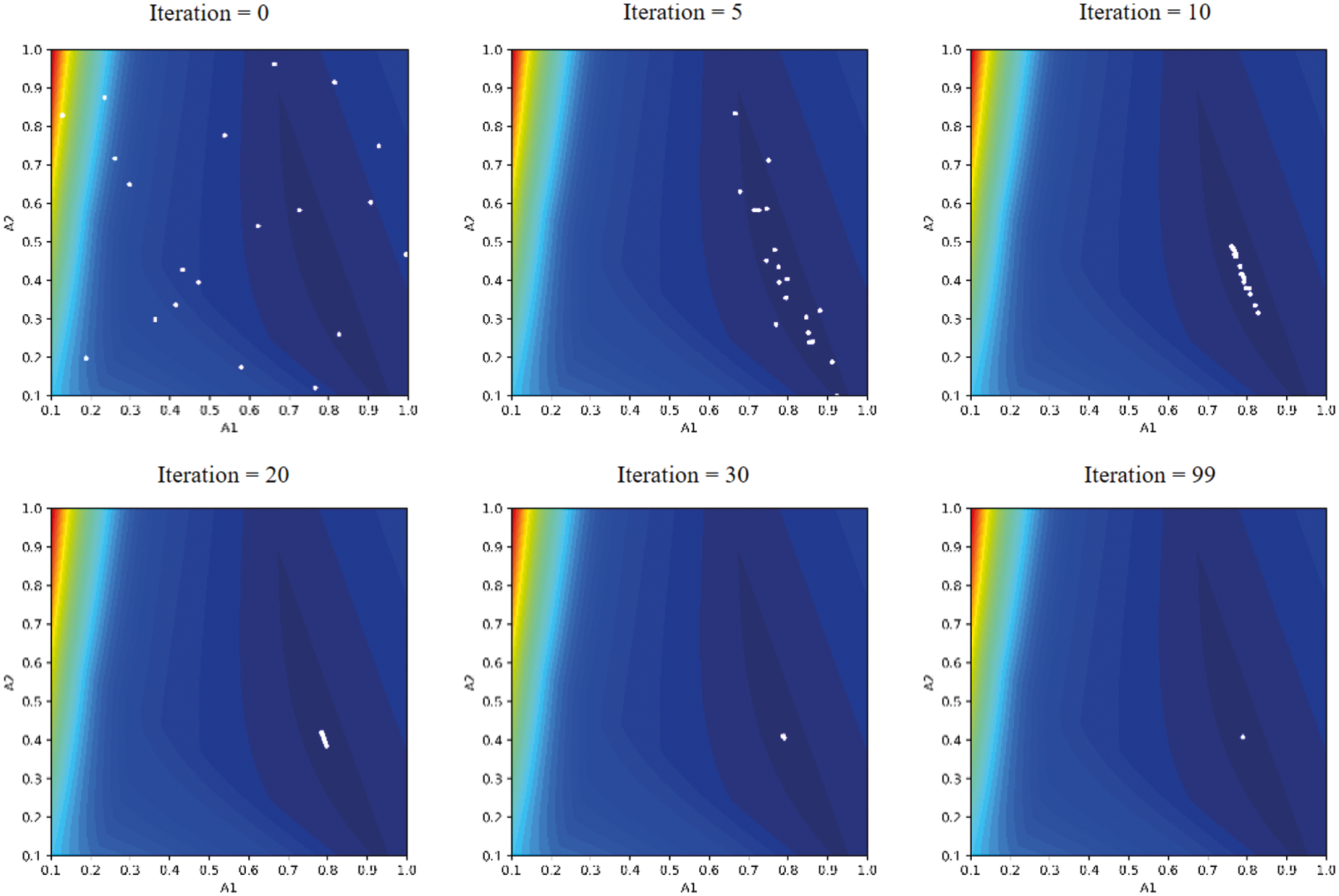
Figure 6: Improvement of the population during the DE optimization process

The optimization parameters F, Cr, max_iter of the CaDE are kept the same as in the DE. The number of iterations for the first phase is set to n_iter1 = 5, meaning the number of samples in the dataset DB is equal to n_iter1 × NP = 5 × 20 = 100. Fig. 7 presents all samples collected in the first phase, where vectors that are labeled +1 are represented as white dots while vectors that are labeled −1 are represented as red dots. Based on the obtained dataset, an AdaBoost classifier is built as the green dashed curve shown in Fig. 7.

Figure 7: Building an AdaBoost classifier based on historical constraint evaluations

In the second phase, the decision of performing exact structural analyses depends on the prediction of the AdaBoost classifier. Fig. 8 illustrates the optimization process of the proposed method at the 5th iteration, in which all white dots represent the target vectors xi(5) of the current population After conducting two operators including mutation and crossover, the machine learning classifier is employed to predict the label of the trial vector ui(5). At this time, one of three possible cases can occur as follows:

Case 1:   If the predicted label ypred_i(5) = +1, the trial individual ui(5) is then checked design constraints using exact structural analysis. These individuals are represented as blue dots in Fig. 8;

Case 2:   If the predicted label ypred_i(5) = −1 and the objective function of the trial vector W(ui(5)) is smaller than or equal to that of the target vector W(xi(5)), it is also checked design constraints using exact structural analysis. These individuals are represented as yellow dots in Fig. 8;

Case 3:   If the predicted label ypred_i(5) = −1 and W(ui(5)) > W(xi(5)), it is eliminated without performing the exact structural analysis. These individuals are marked as magenta dots in Fig. 8.

Figure 8: Illustration of the implementation of the proposed method CaDE

After reaching the stopping condition, the optimal cross-sectional areas of truss members found by the CaDE are A1 = 0.789 cm2 and A2 = 0.408 cm2 which are similar to the results found by the original DE. However, by applying the AdaBoost classifier, the number of exact structural analyses is greatly reduced. The optimization is independently performed 30 times and the statistical results show that the proposed method CaDE requires an average of 1770 structural analyses while the original DE algorithm needs 2000 structural analyses.

4.2 Five Benchmark Truss Problems

4.2.1 Description of the Problems

Five well-known truss sizing optimization problems collected from the literature including the 10-bar planar truss, the 17-bar planar truss, the 25-bar spatial truss, the 72-bar spatial truss, and the 200-bar planar truss are carried out in this section.

The first example considers a simple truss containing 10 members as illustrated in Fig. 9. This structure is made of the material having the modulus of elasticity E = 10,000 ksi and the density ρ = 0.1 lb/in3. This problem has 10 design variables A = {Ai, i = 1, 2,…, 10} where 0.1 in2 ≤ Ai ≤ 33.5 in2 is the cross-sectional areas of ith member. Two vertical loads acting at node (2) and node (4) have the same magnitude P = 100 kips. Stresses inside members must be lower than 25 ksi for both compression and tension. Displacements of nodes (1), (2), (3), (4) are limited within ± 2 in.

Figure 9: Layout of the 10-bar truss

The second example considers a 17-bar planar truss as presented in Fig. 10. This structure is fabricated from a material that has the modulus of elasticity E = 30,000 ksi and the material density ρ = 0.268 lb/in3. Each member in this structure has its own cross-sectional areas and there are 17 design variables in total A = {0.1 in2 ≤ Ai ≤ 33.5 in2, i = 1, 2,…, 17}. A vertical force of 100 kips acts at node (9) of the truss. The allowable stresses in both tension and compression are σallow = 50 ksi and the allowable displacements along the X and Y directions are δallow = 2 in.

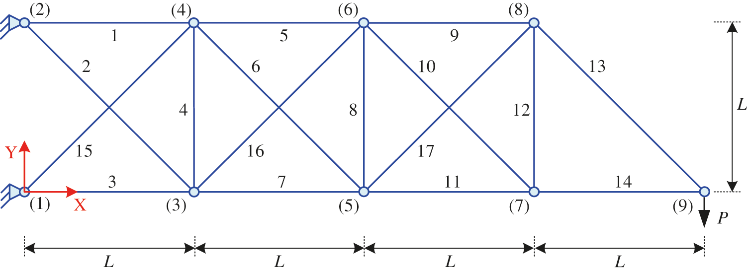
Figure 10: Layout of the 17-bar truss

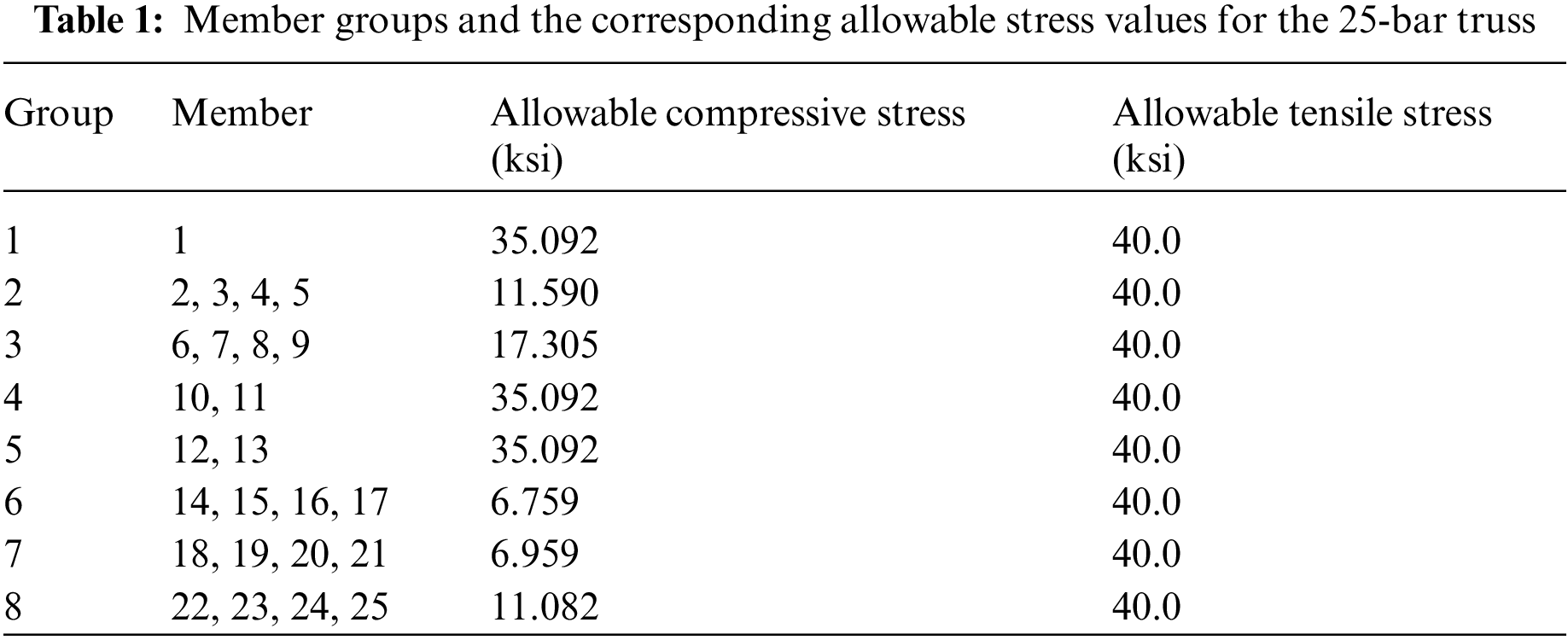
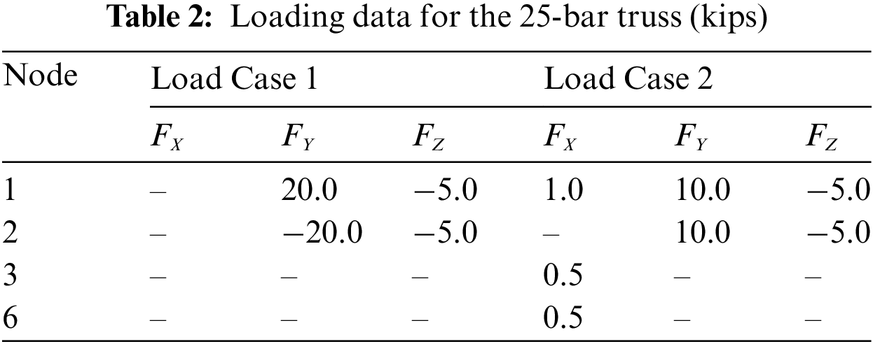
In the third example, a spatial truss containing 25 members as presented in Fig. 11 is considered. This structure is made of the same material as the 10-bar truss (E = 10,000 ksi and ρ=0.1 lb/in3). Members of this structure are classified into 8 groups where members belonging to the same group are assigned the same cross-sectional area that varies between 0.01 in2 to 3.5 in2. This structure is optimized according to both stress constraint and displacement constraint. The allowable stresses are presented in Table 1 and the permissible displacement of all nodes is ±0.35 in. The loading data are shown in Table 2.

Figure 11: Layout of the 25-bar truss

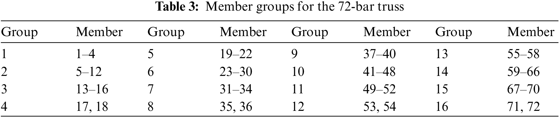
The layout of the 72-bar spatial truss investigated in the fourth example is displayed in Fig. 12. Members are classified into 16 groups as described in Table 3. The minimum and maximum areas of all members are 0.01 in2 and 4.0 in2. Two load cases acting on this structure are as follows: (LC1) two horizontal forces of 5 kips along the X-axis and Y-axis and a vertical force of 5 kips along the opposite direction of the Z-axis act at node (17); (LC2) four vertical forces of 5 kips along the opposite direction of the Z-axis act at four nodes (17), (18), (19), (20), respectively. The design constraints of this problem include stress constraint and displacement constraint. The allowable stresses of all members are ± 25 ksi while the allowable displacements along the X and Y directions are ± 0.25 in.

Figure 12: Layout of the 72-bar truss

The last problem is a 200-bar planar truss which is schematized in Fig. 13. The modulus of elasticity E of the material used in this structure equals 30,000 ksi while the material density ρ equals 0.283 lb/in3. There are three independent load cases as follows:

Figure 13: Layout of the 200-bar truss

(LC1): 1.0 kips acting along the positive x-direction at nodes (1), (6), (15), (20), (29), (34), (43), (48), (57), (62), and (71) (green arrows in Fig. 13);

(LC2): 10 kips acting along the negative y-direction at nodes (1)--(6), (8), (10), (12), (14), (16)--(20), (22), (24), (26), (28)--(34), (36),(38),(40), (42)--(48), (50), (52), (54), (56)--(62), (64), (66), (68), and (70)--(75) (orange arrows in Fig. 13);

(LC3): both (LC1) and (LC2) acting together.

There is no limitation of displacement in this problem. Stresses inside all members must be lower than ± 10 ksi. This structure has 29 groups of members as indicated in Table 4. It means this problem has 29 design variables A = {Ai, i = 1, 2,…, 29} in which Ai represents the cross-sectional area of members belonging the ith group. Ai is limited in the range of [0.1, 15] in2.

4.2.2 Parameter Studies

Obviously, the training dataset size and the number of weak classifiers strongly influence the accuracy of the AdaBoost model, thereby affecting the performance of the proposed method CaDE. In this section, a parametric study is carried out to investigate the influences of these parameters. The 25-bar truss structure described in Section 4.2.1 is taken as the optimization problem for the parametric study.

Firstly, five cases are carried out in which the amount of training samples is set to 100, 500, 1000, 1500, and 2000, respectively. In all cases, the number of weak classifiers used in the AdaBoost model is fixed as T = 100. In the second, four more cases are conducted in which the number of weak classifiers is set to 10, 25, 50, and 200, respectively while the number of training samples is fixed as 1000 data points. There are a total of 9 cases. Other parameters are the same for all cases as follows: the mutation strategy “DE/target-to-best/1”; F = 0.8; Cr = 0.9; NP = 50; and max_iter = 500. Each case is executed 30 times and the results are reported in Table 5.

It can be found that all cases achieve high convergence when the optimal weights found in 30 independent runs are almost the same. However, there is an influence of the parameters on the number of structural analyses that must be conducted during the optimization process. When the training dataset size is fixed to 1000, the case of 10 weak classifiers requires the largest number of structural analyses. When the number of weak classifiers varies from 10 to 100, the number of structural analyses decreases linearly but from 100 to 200, the value of nSA does not change much. When the number of weak classifiers is fixed to 100, the case of 1000 data samples has the fastest convergence speed.

Overall, it is recognized that the pair of parameters: the number of weak classifier T = 100 and the number of training samples = 1000 is a proper selection. This set of parameters is then applied to all further experiments.

4.2.3 Comparison with Regression-Based Surrogate Model

As described in the ‘Introduction’ section, many previous studies have used regression techniques for surrogate modeling. In this section, a comparison is conducted to exhibit the advantage of the classification-based surrogate models. The performances of three optimization methods are evaluated including the original DE method (called the DE), the AdaBoost classifier-assisted DE method (called the CaDE), and the AdaBoost regression-assisted DE method (called the RaDE).

The details of the DE and the CaDE are already introduced in Section 2.1 and Section 3.2. The RaDE has also two phases: the model building phase and the model employing phase. In the model building phase, the original DE algorithm is employed as usual and all solutions are exactly evaluated through structural analyses and the degree of constraint violation of each solution is saved in the database. After n_iter1 iterations, an AdaBoost regression model is trained with the obtained dataset with the aim of predicting the constraint violation degree of a new solution. Then, the trained model is employed instead of the constraint verification in the second stage.

Five optimization problems mentioned in Section 4.2.1 are solved using three methods DE, CaDE, RaDE, respectively. The setting parameters for these methods are summarized in Table 6. Each problem is solved 30 independent times, and the statistical results including best, mean, worst, and standard deviation (SD) are reported in Table 7. The average number of structural analyses conducted during the optimization process (nSA) as well as the degree of constraint violation (cv) are also presented.

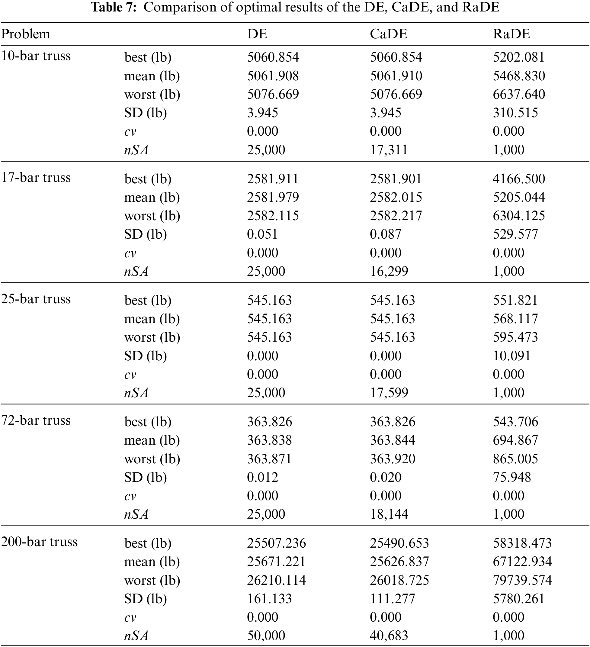
Based on the results in Table 7, some observations can be pointed out as follows. First of all, it can be seen that the optimal designs found by the CaDE are very similar to the DE but the CaDE needs fewer structural analyses than the DE. For the four first problems, the DE requires 25000 structural analyses and for the last problem, the DE requires 50000 structural analyses. However, the required number of structural analyses of the CaDE for five problems are 17311 times, 16299 times, 17599 times, 18144 times, and 40683 times, respectively.

Secondly, the required numbers of structural analyses of the RaDE for all problems are very small compared to the DE and the CaDE. This method conducts only 1000 times of exact structural analyses to generate the training data. However, due to the error between the structural analyses and the surrogate modeling, the optimal designs found by the RaDE are not good. Although these designs do not violate design constraints, the weights of these designs are much greater than the optimal designs found by the DE and the CaDE.

In general, using the regression-based surrogate modeling significantly reduces the number of structural analyses during the optimization process but the obtained results are not the global optimal. Otherwise, the classification-based surrogate modeling only reduces the number of structural analyses by about 25%, but the advantage of this method is that it retains the search performance of the original DE method.

4.2.4 Comparison with Other DE Variants

Furthermore, the results of these problems found by other DE variants are introduced for comparison. Four DE variants collected in the literature [40] include the composite differential evolution (CoDE), the self-adaptive control parameters differential evolution (JDE), the adaptive differential evolution with optimal external archive (JADE), and the self-adaptive differential evolution (SADE). The statistical results are introduced in Table 8.

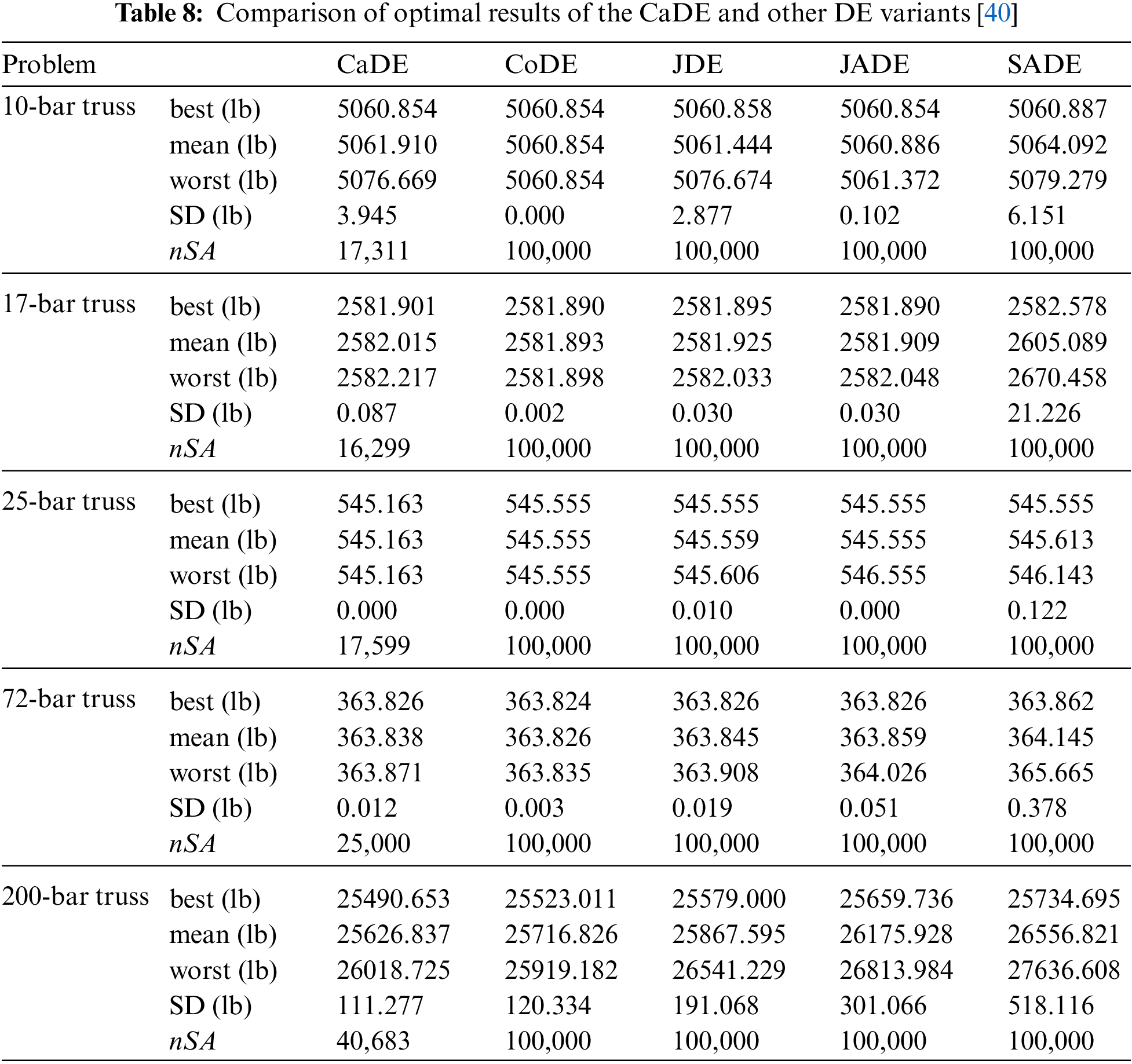
For the 10-bar truss, the optimal design of the CaDE is similar to the CoDE and JADE and better than the JDE and the SADE. For the 17-bar truss, the optimal weight found by the CaDE is very similar to those of the DE variants. For the third problem of the 25-bar truss, the minimum weight of the CaDE (545.163 lb) is lower than those of other DE variants (545.555 lb). For the fourth problem of the 72-bar truss, the optimal weights found by the CaDE, the JDE, the JADE are the same (363.826 lb) and this value is slightly larger than the optimal weight obtained by the CoDE (363.824 lb). For the last problem, the weight of the 200-bar truss received from the CaDE is the smallest value (25490.653 lb), followed by the CoDE (25523.011 lb), the JDE (25579.000 lb), the JADE (25659.736 lb), and the SADE (25734.695 lb). Moreover, the smaller value of the standard deviation of the CaDE (111.277 lb) in comparison with the remaining algorithms (120.334 lb for the CoDE, 191.068 lb for the JDE, 301.116 for the JADE, and 518.116 lb for the SADE) indicates the reliability of the proposed method.

In terms of the convergence speed, the CaDE exhibits its superior. The CaDE requires from 16299 to 40683 structural analyses while the remaining methods conduct 100000 structural analyses for finding the optimal results. It is apparent that the CaDE is more speedy than the CoDE, the JDE, the JADE, and the SADE.

4.3 A Real-Size Transmission Tower

In this section, the CaDE is employed to optimize the weight of a real-size transmission tower for showing its applicability in the practical design. This tower consists of 244 members which are classified into 32 groups as presented in Fig. 14. Members belonging to the same group have the same cross-section which is chosen from 64 equal angle profiles from L35 × 3 to L200 × 25. It means this problem is a discrete optimization. The steel material used in this structure has mechanical properties as follows: the weight density ρ = 7850 kg/m3; the modulus of elasticity E = 210,000 N/mm2; the yield strength Fy = 233.3 N/mm2. This structure is designed according to the AISC-ASD specification in which the tensile stress constraint is as follows:

σt≤[σ]t=0.6Fy(21)

where: σt is the tensile stress of the member; [σ]t is the allowable tensile stress; Fy is the yield strength.

Figure 14: Layout of the transmission tower

The buckling stress constraint is as follows:

σc≤[σ]b={(Fy(1−λ2Cc2))/(Fy(1−λ2Cc2))(53+3λ8Cc−λ38Cc)(53+3λ8Cc−λ38Cc)ifλ<Cc12π2E23λ2ifλ≥Cc(22)

where: σc is the compressive stress of the member; [σ]b is the allowable buckling stress; λ=KL/r is the maximum slenderness ratio of the member; K is the effective length factor which equals 1 in this case; L is the length of the member; and r is the radius of gyration of the member's cross-section; Cc is the slenderness ratio dividing the elastic and inelastic buckling regions which is determined using the following formula:

Cc=2π2EFy(23)

Additionally, the maximum slenderness ratio λ is limited to 200 for compression members while 300 for tension members. The tower is subjected to two independent load cases. Table 9 presents the force magnitudes of two applied load cases and the corresponding displacement limitation.

This structure is optimized according to both the DE and the CaDE with the same parameters as follows: NP = 50; F = 0.8; Cr = 0.9; max_iter = 1000. The number of iterations for the first phase is set to n_iter1 = 300 which means 15000 samples have been collected for the training dataset. The statistical results obtained by the DE and the CaDE are presented in Table 10. The minimum weight of the tower found by the DE and the CaDE are the same (6420.652 kg) but other statistical results of the CaDE including mean, worst, and SD are smaller than those of the DE, indicating the stability of the proposed method. The number of structural analyses of the CaDE is only 24865 times, which is about 50% of the number of structural analyses performed by the DE. In other words, the CaDE omits about half of useless structural analyses. This is clearly shown in Fig. 15.

Figure 15: Comparison of the DE and the CaDE for the transmission tower problem

4.4 Evaluation of the Effectiveness of the Proposed Method CaDE

The average numbers of structural analyses (nSA) conducted in the six investigated examples as well as the reduction rates when using the AdaBoost classifier are listed in Table 11. Furthermore, the computing times of the DE and the CaDE are also reported.

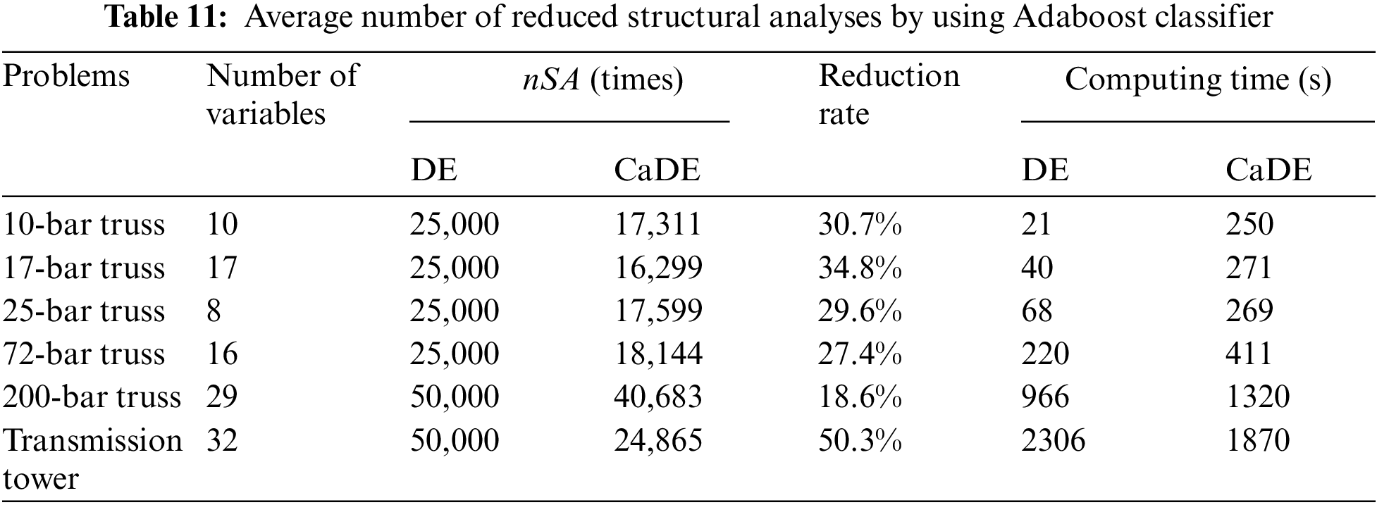
It is clearly seen that the application of the AdaBoost classifier into the optimization process helps to reduce the number of structural analyses. Specifically, the CaDE has reduced the number of structural analyses by up to 50.3% for the transmission tower problem. The minimum reduction rate is 18.6% for the 200-bar truss problem.

In contrast, the CaDE is slower than the DE in five benchmark truss problems when compared in terms of time. The CaDE is only faster than the DE in the transmission tower problem. This is because integrating the AdaBoost classifier into the DE increases the complexity of the algorithm. Moreover, the CaDE requires additional time for training and employing the AdaBoost model. However, for the transmission tower, this additional time is small in comparison with the computational time of fitness evaluation where involving structural analysis. Therefore the total computing time of the CaDE is lower than that of the DE in this case. In general, it can be concluded that the proposed method is effective with large-scale structures.

5  Conclusions

In this paper, the AdaBoost classifier-assisted Differential Evolution method, called CaDE, is proposed for optimizing the weight of truss structures. By integrating the AdaBoost classification technique into the DE algorithm, the unnecessary structural analyses are significantly reduced. More specifically, in the early generations, the original Differential Evolution algorithm is deployed but the data generated in this phase is collected to train an AdaBoost model with the aim of classifying the safety state of structures. In later generations, this model is used to detect and eliminate unpromising individuals.

Through five optimization problems of truss structures, the CaDE method is proved to be a robust and reliable algorithm. In most cases, the CaDE method accomplishes the optimal results as good as or better than those of other algorithms in the literature but the numbers of structural analyses performed by the CaDE method are lower than those performed by the original DE algorithm. Besides advantages, the proposed method has also some drawbacks. Firstly, it is more complex than the original DE algorithm. Moreover, the proposed method requires more computational time for training and employing the machine learning model. Therefore, it is suitable for large-scale structures in which the structural analysis task is very time-consuming.

In the future, the application of the CaDE method can be extended for other types of structures. Furthermore, using machine learning models to improve the performance of other optimization algorithms also forms an interesting research topic.

Acknowledgement: The authors gratefully acknowledge the financial support provided by HUCE. Besides, the first author T. H. N. would also like to thank VINIF for the support.

Funding Statement: This research is funded by Hanoi University of Civil Engineering (HUCE) in Project Code 35-2021/KHXD-TĐ.

Conflicts of Interest: The authors declare that they have no conflicts of interest to report regarding the present study.

References

1. Jenkins, W. M. (1991). Towards structural optimization via the genetic algorithm. Computers & Structures, 40(5), 1321–1327. DOI 10.1016/0045-7949(91)90402-8. [Google Scholar] [CrossRef]
2. Rajeev, S., Krishnamoorthy, C. S. (1992). Discrete optimization of structures using genetic algorithms. Journal of Structural Engineering, 118(5), 1233–1250. DOI 10.1061/(ASCE)0733-9445(1992)118:5(1233). [Google Scholar] [CrossRef]
3. Cai, J., Thierauf, G. (1996). Evolution strategies for solving discrete optimization problems. Advances in Engineering Software, 25(2–3), 177–183. DOI 10.1016/0965-9978(95)00104-2. [Google Scholar] [CrossRef]
4. Papadrakakis, M., Lagaros, N. D., Thierauf, G., Cai, J. (1998). Advanced solution methods in structural optimization based on evolution strategies. Engineering Computations, 15(1), 12–34. DOI 10.1108/02644409810200668. [Google Scholar] [CrossRef]
5. Wang, Z., Tang, H., Li, P. (2009). Optimum design of truss structures based on differential evolution strategy. 2009 International Conference on Information Engineering and Computer Science, Wuhan, China, IEEE. [Google Scholar]
6. Wu, C. Y., Tseng, K. Y. (2010). Truss structure optimization using adaptive multi-population differential evolution. Structural and Multidisciplinary Optimization, 42(4), 575–590. DOI 10.1007/s00158-010-0507-9. [Google Scholar] [CrossRef]
7. Camp, C. V., Meyer, B. J., Palazolo, P. J. (2004). Particle swarm optimization for the design of trusses. Structures 2004: Building on the Past, Securing the Future, Structure Congress 2004, Nashville, Tennessee, USA, ASCE. [Google Scholar]
8. Perez, R. L., Behdinan, K. (2007). Particle swarm approach for structural design optimization. Computers & Structures, 85(19–20), 1579–1588. DOI 10.1016/j.compstruc.2006.10.013. [Google Scholar] [CrossRef]
9. Sonmez, M. (2011). Artificial Bee colony algorithm for optimization of truss structures. Applied Soft Computing, 11(2), 2406–2418. DOI 10.1016/j.asoc.2010.09.003. [Google Scholar] [CrossRef]
10. Lee, K. S., Geem, Z. W. (2004). A new structural optimization method based on the harmony search algorithm. Computers & Structures, 82(9–10), 781–798. DOI 10.1016/j.compstruc.2004.01.002. [Google Scholar] [CrossRef]
11. Lee, K. S., Han, S. W., Geem, Z. W. (2011). Discrete size and discrete-continuous configuration optimization methods for truss structures using the harmony search algorithm. Iran University of Science & Technology, 1(1), 107–126. [Google Scholar]
12. Degertekin, S. O., Hayalioglu, M. S. (2013). Sizing truss structures using teaching-learning-based optimization. Computers & Structures, 119, 177–188. DOI 10.1016/j.compstruc.2012.12.011. [Google Scholar] [CrossRef]
13. Camp, C. V., Farshchin, M. (2014). Design of space trusses using modified teaching–learning based optimization. Engineering Structures, 62, 87–97. DOI 10.1016/j.engstruct.2014.01.020. [Google Scholar] [CrossRef]
14. Kaveh, A., Mahdavi, V. R. (2014). Colliding bodies optimization method for optimum design of truss structures with continuous variables. Advances in Engineering Software, 70, 1–12. DOI 10.1016/j.advengsoft.2014.01.002. [Google Scholar] [CrossRef]
15. Kaveh, A., Mahdavi, V. R. (2014). Colliding bodies optimization method for optimum discrete design of truss structures. Computers & Structures, 139, 43–53. DOI 10.1016/j.compstruc.2014.04.006. [Google Scholar] [CrossRef]
16. Degertekin, S. O. (2012). Improved harmony search algorithms for sizing optimization of truss structures. Computers & Structures, 92, 229–241. DOI 10.1016/j.compstruc.2011.10.022. [Google Scholar] [CrossRef]
17. Bureerat, S., Pholdee, N. (2016). Optimal truss sizing using an adaptive differential evolution algorithm. Journal of Computing in Civil Engineering, 30(2), 04015019. DOI 10.1061/(ASCE)CP.1943-5487.0000487. [Google Scholar] [CrossRef]
18. Ho-Huu, V., Nguyen-Thoi, T., Vo-Duy, T., Nguyen-Trang, T. (2016). An adaptive elitist differential evolution for optimization of truss structures with discrete design variables. Computers & Structures, 165, 59–75. DOI 10.1016/j.compstruc.2015.11.014. [Google Scholar] [CrossRef]
19. Pham, H. A. (2016). Truss optimization with frequency constraints using enhanced differential evolution based on adaptive directional mutation and nearest neighbor comparison. Advances in Engineering Software, 102, 142–154. DOI 10.1016/j.advengsoft.2016.10.004. [Google Scholar] [CrossRef]
20. Papadrakakis, M., Lagaros, N. D., Tsompanakis, Y. (1998). Structural optimization using evolution strategies and neural networks. Computer Methods in Applied Mechanics and Engineering, 156(1–4), 309–333. DOI 10.1016/S0045-7825(97)00215-6. [Google Scholar] [CrossRef]
21. Papadrakakis, M., Lagaros, N. D., Tsompanakis, Y. (1999). Optimization of large-scale 3-D trusses using evolution strategies and neural networks. International Journal of Space Structures, 14(3), 211–223. DOI 10.1260/0266351991494830. [Google Scholar] [CrossRef]
22. Salajegheh, E., Gholizadeh, S. (2005). Optimum design of structures by an improved genetic algorithm using neural networks. Advances in Engineering Software, 36(11–12), 757–767. DOI 10.1016/j.advengsoft.2005.03.022. [Google Scholar] [CrossRef]
23. Taheri, F., Ghasemi, M. R., Dizangian, B. (2020). Practical optimization of power transmission towers using the RBF-based ABC algorithm. Structural Engineering and Mechanics, 73(4), 463–479. DOI 10.12989/sem.2020.73.4.463. [Google Scholar] [CrossRef]
24. Hosseini, N., Ghasemi, M. R., Dizangian, B. (2022). ANFIS-based optimum design of real power transmission towers with size, shape and panel variables using BBO algorithm. IEEE Transactions on Power Delivery, 37(1), 29–39. DOI 10.1109/TPWRD.2021.3052595. [Google Scholar] [CrossRef]
25. Nguyen, T. H., Vu, A. T. (2020). Using neural networks as surrogate models in differential evolution optimization of truss structures. International Conference on Computational Collective Intelligence, Switzerland, Springer. [Google Scholar]
26. Mai, H. T., Kang, J., Lee, J. (2021). A machine learning-based surrogate model for optimization of truss structures with geometrically nonlinear behavior. Finite Elements in Analysis and Design, 196, 103572. DOI 10.1016/j.finel.2021.103572. [Google Scholar] [CrossRef]
27. Kaveh, A., Gholipour, Y., Rahami, H. (2008). Optimal design of transmission towers using genetic algorithm and neural networks. International Journal of Space Structures, 23(1), 1–19. DOI 10.1260/026635108785342073. [Google Scholar] [CrossRef]
28. Chen, T. Y., Cheng, Y. L. (2010). Data-mining assisted structural optimization using the evolutionary algorithm and neural network. Engineering Optimization, 42(3), 205–222. DOI 10.1080/03052150903110942. [Google Scholar] [CrossRef]
29. Kramer, O., Barthelmes, A., Rudolph, G. (2009). Surrogate constraint functions for CMA evolution strategies. Annual Conference on Artificial Intelligence, Germany, Springer. [Google Scholar]
30. Poloczek, J., Kramer, O. (2013). Local SVM constraint surrogate models for self-adaptive evolution strategies. Annual Conference on Artificial Intelligence, Germany, Springer. [Google Scholar]
31. Wang, H., Jin, Y. (2018). A random forest-assisted evolutionary algorithm for data-driven constrained multiobjective combinatorial optimization of trauma systems. IEEE Transactions on Cybernetics, 50(2), 536–549. DOI 10.1109/TCYB.6221036. [Google Scholar] [CrossRef]
32. Freund, Y., Schapire, R. E. (1997). A Decision-theoretic generalization of on-line learning and an application to boosting. Journal of Computer and System Sciences, 55(1), 119–139. DOI 10.1006/jcss.1997.1504. [Google Scholar] [CrossRef]
33. Nguyen, T. H., Vu, A. T. (2021). Evaluating structural safety of trusses using machine learning. Frattura ed Integrità Strutturale, 15(58), 308–318. DOI 10.3221/IGF-ESIS.58.23. [Google Scholar] [CrossRef]
34. Storn, R., Price, K. (1997). Differential evolution–A simple and efficient heuristic for global optimization over continuous spaces. Journal of Global Optimization, 11(4), 341–359. DOI 10.1023/A:1008202821328. [Google Scholar] [CrossRef]
35. Das, S., Suganthan, P. N. (2010). Differential evolution: A survey of the state-of-the-art. IEEE Transactions on Evolutionary Computation, 15(1), 4–31. DOI 10.1109/TEVC.2010.2059031. [Google Scholar] [CrossRef]
36. Das, S., Mullick, S. S., Suganthan, P. N. (2016). Recent advances in differential evolution–An updated survey. Swarm and Evolutionary Computation, 27, 1–30. DOI 10.1016/j.swevo.2016.01.004. [Google Scholar] [CrossRef]
37. Charalampakis, A. E., Tsiatas, G. C. (2019). Critical evaluation of metaheuristic algorithms for weight minimization of truss structures. Frontiers in Built Environment, 5. DOI 10.3389/fbuil.2019.00113. [Google Scholar] [CrossRef]
38. Pedregosa, F., Varoquaux, G., Gramfort, A., Michel, V., Thirion, B., et al. (2011). Scikit-learn: Machine learning in Python. The Journal of Machine Learning Research, 12, 2825–2830. [Google Scholar]
39. Ferreira, A. J. (2009). MATLAB codes for finite element analysis. Netherlands: Springer. [Google Scholar]
40. Georgioudakis, M., Plevris, V. (2020). A comparative study of differential evolution variants in constrained structural optimization. Frontiers in Built Environment, 6. DOI 10.3389/fbuil.2020.00102. [Google Scholar] [CrossRef]
Cite This Article
Copyright © 2023 The Author(s). Published by Tech Science Press.
This work is licensed under a Creative Commons Attribution 4.0 International License , which permits unrestricted use, distribution, and reproduction in any medium, provided the original work is properly cited.
Downloads
Citation Tools