Shape and Size Optimization of Truss Structures under Frequency Constraints Based on Hybrid Sine Cosine Firefly Algorithm

1  Introduction

Since the natural frequency has an important influence on the vibration of the structural system, it is necessary to constrain the natural frequency in the structural design to avoid resonance and damage. Bellagamba et al. [1] presented the seminal work on frequency constrained truss shape and size optimization, and since then researches in this area have developed rapidly over the past 30 years.

The structural optimization with frequency constraints aims to minimize the weight of the structure while ensuring the satisfaction of frequency constraints. Nevertheless, frequency constraints are highly nonlinear, nonconvex and implicit with respect to the design variables [2]. Moreover, the mixture of shape and size variables can cause severe mathematical difficulties and divergence because of the different magnitude orders. The characteristics of the optimization problem limit the application of gradient-based algorithms in this field [3,4]. Consequently, non-gradient-based algorithms, especially metaheuristic algorithms were developed to deal with this problem. These algorithms use stochastic searching techniques to select potential solutions, which have better global search ability with fewer limitations in application [5–7]. However, metaheuristic algorithms still have some drawbacks such as time-consuming search and expensive computational cost.

Firefly algorithm (FA) is one of the nature-inspired metaheuristic algorithms based on the flashing patterns and social behavior of fireflies, and it can be considered as a generalization to particle swarm optimization (PSO), differential evolution, and simulated annealing algorithms through parameter adjustment [8,9]. Therefore, FA inherits the advantages of the three algorithms and shows an impressive performance. Benefiting from the excellent global search ability, FA was successfully applied to various fields [10–12]. However, the computational cost of FA is still expensive, and the exploitation ability has the potential for progress. Accordingly, different algorithms and techniques were combined with FA for improvements [13–16]. These results confirmed that such hybrid algorithms outperformed the standard algorithms in terms of solution accuracy and convergence rate. Nevertheless, how to simplify the computational complexity of FA is still an unsolved problem.

Sine cosine algorithm (SCA) [17] is a recently developed metaheuristic algorithm, which uses the characteristics of sine and cosine trigonometric functions in the search process to solve global optimization problems. SCA has competitive performance compared with other algorithms [18–21]. As SCA updates each candidate solution using the information of the global optimal solution, the exploitation ability and convergence rate are impressive. However, SCA faces some difficulties like falling into local optima and skipping of true solutions. Furthermore, SCA has not been applied to shape and size optimization problems of truss structures.

In this paper, the computational complexity of FA is reduced and a hybrid sine cosine firefly algorithm (HSCFA) with adaptive penalty function is proposed to deal with shape and size optimization of truss structures with frequency constraints. HSCFA takes advantage of SCA, FA, and Lévy flight to achieve a better balance between exploration and exploitation.

The remainder of this article is organized as follows. The mathematical model of the discrete structural optimization problem is presented in Section 2. The introductions of SCA, FA, Lévy flight-based local search technique, elitist selection technique and self-adaptive penalty function are given in Section 3. HSCFA is proposed in Section 4. The efficiency of HSCFA is evaluated in Section 5. Finally, the main conclusions are summarized in Section 6.

2  Mathematical Model of Optimization Problems

Generally, shape and size optimization for truss structures aims to minimize the weight while satisfying functional constraints. The design variables include the cross-sectional area of the members and the nodal positions of the critical members. Thus, the mathematical model can be expressed as the following Eq. (1).

Minimize W=∑i=1nρiAiLi(xq)Subject to:ωj≤ωj,maxωl≥ωl,minAi,min≤Ai≤Ai,max,i=1,2,…,nxq,min≤xq≤xq,max,q=1,2,…,m(1)

where W is the weight of the structure. For each member i, ρi means the material density, Ai indicates the cross-sectional area, Li is the length, xq is the nodal positions. n and m are the number of members and nodes, respectively. ωj and ωj,max are the j-th natural frequency and its corresponding upper bound. ωl and ωl,min are the l-th natural frequency and its corresponding lower bound. Ai,min and A i,max are the lower and upper bounds of Ai. xq,min and xq,max are the lower and upper bounds of xq.

3  Preliminaries

3.1 Firefly Algorithm

FA was developed by Yang in 2008 [22], and it was inspired by the social behavior of firefly. In FA, three idealized rules are made including all fireflies are unisex, attractiveness is proportional to the brightness, and brightness is proportional to the value of the objective function. Then, the mathematical imitation of light intensity is settled. Obviously, the distance and air absorption affect the variation of light intensity, and the firefly’s attractiveness is proportional to the light intensity seen by adjacent fireflies. Therefore, the attractiveness β is formulated as the following Eq. (2).

β(r)=β0e−γrij2(2)

where β0 is the attractiveness of r = 0. The light absorption coefficient γ indicates the strength of the attraction. In general, γ distributes in [0.01,100]. The distance rij between fireflies i and j is defined as the following Eq. (3).

rij=‖Xi−Xj‖=∑k=1d(Xi,k−Xj,k)2(3)

The movement of firefly i is calculated by the following Eq. (4).

Xit+1=Xit+β0e−γrij2(Xjt−Xit)+α(rand−12)(4)

where Xit is the position of the i-th firefly at t-th iteration. α and ‘rand’ are the randomization parameter that take from [0,1]. α is a constant that adjusts the random step of FA, and ‘rand’ is a random vector usually generated by Gaussian distribution, uniform distribution, and so on.

3.2 Sine Cosine Algorithm

SCA is a novel population-based optimization algorithm proposed by Mirjalili [17]. SCA updates the movement of the search agents toward the best solution using a mathematical model based on sine and cosine functions. In SCA, the following Eq. (5) is used for both exploration and exploitation.

Xit+1={Xit+r1×sin⁡(r2)×|r3Pt−Xit|,r4<0.5Xit+r1×cos⁡(r2)×|r3Pt−Xit|,r4≥0.5(5)

where Xit is the position of the i-th solution at t-th iteration. Pt means the best solution at t-th iteration. r1 is distributes in [0,2]. r2 can be taken from [0,2π]. r3 is a random number in [0,2]. It can determine the effect of destination Pt on the current movement. The parameter r3 brings a random weight for the destination to stochastically emphasize (r3 > 1) or deemphasize (r3 < 1) the effect of destination in defining the distance. r4 is a random number in [0,1] that decides the switch between sine and cosine components. The range of sine and cosine changes adaptively as the following Eq. (6).

r1=a(1−t/T)(6)

where t and T are the current and maximum iteration. a is a positive constant. The search range of SCA is illustrated in Fig. 1 with a = 2 [17].

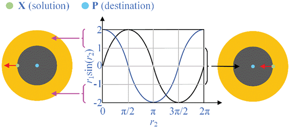
Figure 1: Search range of SCA

From Eq. (5) and Fig. 1, the next position is inside the space between X and P when the values of r1sin(r2) are in [–1,1]. And it will be outside the space between X and P when the values of r1sin(r2) are in (1,2] and [–2, –1). Thus, both r1 and r2 determine the movement distance and search space.

3.3 Lévy Flight-Based Search Technique

Lévy flight was a non-Gaussian random process proposed by Chechkin et al. [23] in 2008, and its random walk is obtained by Lévy distribution. The direction of the flight is random, but the steps are distributed as a power function. Lévy flight has been successfully used to improve the heuristic algorithms due to its strong random search capability [24,25]. The Lévy distribution is generally expressed as L(s)∼|s|−1−β, where s is distributed within the interval (0,2). Its mathematical expression is defined as the following Eq. (7) [26].

L(s,γ,μ)={γ2πexp⁡[−γ2(s−μ)]1(s−μ)3/2if 0<μ<s<∞,0otherwise(7)

where s, γ and μ are step size, control parameter of distribution scale and transmission parameter respectively. The Fourier transform of Lévy flight can be expressed as the following Eq. (8).

Lévy(β)=exp⁡[−α|k|β],0<β≤2(8)

where α∈[–1,1]. The stability factor β is also known as the Lévy index and distributes in (0,2). The step size s can be determined by the Mantegna algorithm as the following Eq. (9).

s=u|v|1/β(9)

where u and v have Gaussian distribution as the following Eqs. (10) and (11).

u∼N(0,σu2),v∼N(0,σv2)(10)

σu={Γ(1+β)sin⁡(πβ/2)Γ[(1+β)/2]∗β∗2(β−1)/2}(1/β),σv=1(11)

where Γ(z) is a gamma function that can be defined as the following Eq. (12).

Γ(z)=∫0∞tz−1ekdk(12)

Then, the Lévy flight-based local search technique can be defined as the following Eq. (13).

Xit+1=Xit+Xit⊕Lévy(β), if Q=NgorNs=Na(13)

where ⊕ denotes Hadamard product. The values of the stagnation times of the particle Ns and the number of constraint violation Q are evaluated before updating the solution. The number of constraint functions Ng and the allowable stagnation times Na are constants. The solutions will be updated by Eq. (13), when Q = Ng or Ns = Na.

3.4 Elitist Selection Technique

The elitist selection technique was proposed for the selection progress [27]. This mechanism is performed as follows: firstly, the last generation of population is combined with this generation of population to create a new group of population. Then, reorder the new population according to the fitness value. Choose the best half individuals of the new population to construct the population for the next generation. In this way, the better population of the two generations is always stored for the next generation. This technique helps the algorithm eliminate the poor individuals and obtain a better convergence rate.

3.5 Self-Adaptive Penalty Function

The penalty function method is one of the most popular constraint handling techniques [28,29]. Based on this method, Tao et al. [12] proposed a self-adaptive penalty function strategy to solve constrained optimization problems. The fitness function is written as the following Eqs. (14)–(16).

F(X)=f(X)+Q∑i=1Qh(t)gi(X)f(X)(14)

{gi(X)=|σi/σiall−1| if ith constraint violatedgi(X)=0 if ith constraint satified(15)

h(t)=1+t/T(16)

where gi(X) is the ith normalized constraint function. σi and σiall are the actual value and allowable value of ith constraint, h(t) is the penalty parameter. The value of penalty function will increase with the increase of iterations, violation number and violation degree. It also makes sure that the second item of Eq. (14) has the same dimension and order of magnitude as the objective function.

4  Proposed New Developments

Generally, the accuracy of the optimal solution and the computational cost are two core indices to evaluate the performance of metaheuristic algorithms. In this section, HSCFA is proposed to enhance the solution accuracy and computational cost of FA.

4.1 Modified Firefly Algorithm

4.1.1 Motivation

The full attraction model defines the movement of fireflies in FA during the search process [30]. In this model, one firefly is attracted by all other brighter fireflies. Moreover, the brightest one is not attracted by any firefly, and the darkest firefly is attracted by all other fireflies. The full attraction model is represented in Fig. 2, in which both the volume and the luminous organ relate to the brightness of the firefly. The larger the volume is, the brighter the firefly is.

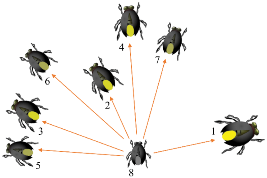
Figure 2: Attraction model among fireflies

As shown in Fig. 2, firefly 8 is the darkest one, and firefly 1 is the brightest one. The seven brighter fireflies are attractive to the firefly 8, and no firefly is attractive to firefly 1. Thus, firefly 8 is hard to approach to the brightest firefly 1 with such an attraction model. To further investigate the attraction model, the real update formula for firefly 8 is given as shown in Eq. (17).

X8t+1=7⋅X8t+∑j=17β0e−γr8j2(Xjt−X8t)+7⋅α(rand−12)(17)

If the value of Xjt is larger than X8t, the value of X8t+1 is far larger than X8t. Thus, the value of X8t+1 is easily beyond the upper bound of the design variable. Then, the value of X8t+1 will be automatically adjusted to the upper bound based on the boundary control method of FA. This makes it difficult for the algorithm to obtain a variety of solutions.

The distance rij between fireflies i and j is affected by the different magnitude orders of the variables, especially for the shape and size optimization problems. If the value of r is always large, it will affect the convergence of the algorithm. In order to further investigate the change of r through the iteration, benchmark functions with different design variable spaces are tested. The mathematical definition, search range and global minimum are listed in Table 1. The changes of the distance r during the search process are illustrated in Fig. 3. In the test, n = 5 and d = 5.

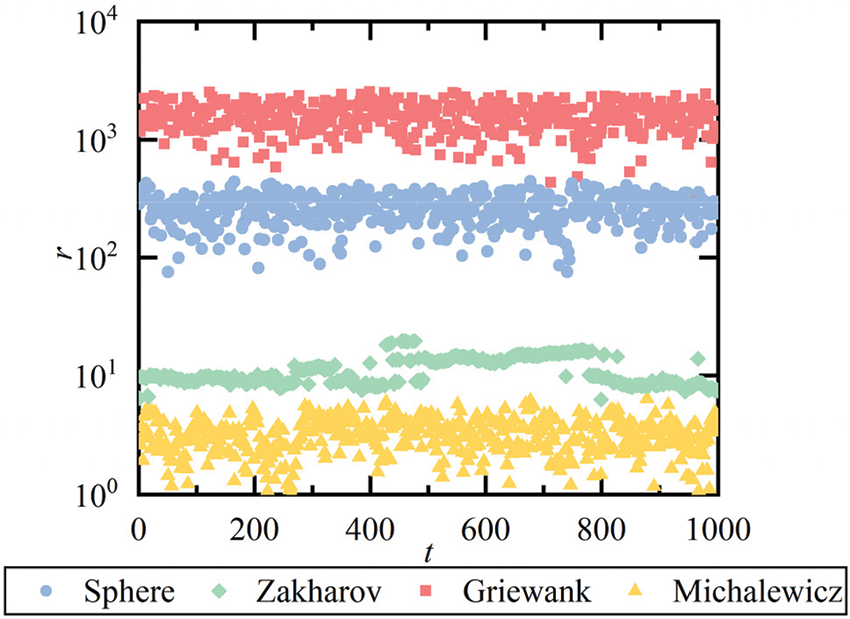
Figure 3: The changes of distance r

From Fig. 3, the values of r are different with varying search ranges. According to Eq. (2), the influence of different magnitude orders should be eliminated in the calculation of r to ensure the effectiveness of the algorithm for different structural optimization problems.

Moreover, it also can be concluded from the full attraction model that the total number of attractions at each generation for population n is n(n–1)/2. Let O(f) be the computational time complexity of the fitness evaluation function f(·) [31]. The Firefly algorithm contains an external loop based on the number of algorithm iterations T and two internal cycles based on the population number n, so the computational time complexity of the standard FA is O(T · n2 · f).

4.1.2 Modification

Although the attraction can enhance the exploitation ability, too many attractions on a firefly lead to uncertain search direction and weaken the exploitation ability. Therefore, the attraction model is modified and only one solution in the top three is selected to update the worse solutions to reduce the time complexity. Furthermore, the search range is introduced into the calculation of r to address the different magnitude orders of the mixed variables. In addition, the fixed randomization parameter α slows down the convergence, and the redundant parameters of a hybrid algorithm will increase the difficulty of the algorithm’s operation. Thus, r1 of SCA is utilized to replace α of FA to accelerate the convergence. Eqs. (3) and (4) can be modified as the following Eqs. (18) and (19).

rij=∑k=1d(Xi,k−Xj,k)2(Ubk−Lbk)2(18)

Xit+1=Xit+β0e−γrrj2(Xrt−Xit)+r1(rand−12)(19)

where Ubk and Lbk are the upper and lower bound of kth variable. Xrt is randomly selected one of the top three fireflies. In the modified FA (MFA), the total number of attractions at each generation is n. Consequently, the time complexity is reduced to O (T · n · f). The changes of the distance r of MFA are illustrated in Fig. 4. In the test, n = 5 and d = 5.

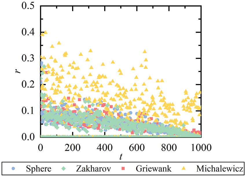
Figure 4: The changes of distance r

From Fig. 4, the values of r are distributed in [0,0.5]. Therefore, the different magnitude orders of variables are conquered by the modification to fit different structural optimization problems.

4.2 Hybrid Sine Cosine Firefly Algorithm (HSCFA)

A hybrid sine cosine firefly algorithm (HSCFA) integrating modified FA, SCA, Lévy flight and adaptive penalty function is proposed in this section. HSCFA takes advantage of modified FA’s exploration ability, SCA’s exploitation ability, and Lévy flight’s strong random search ability. In order to ensure varied population diversity, the population is divided into two equivalent parts that used modified FA and SCA for solution update respectively. The random search strategy based on Lévy flight is employed to update the solutions that stagnate for several iterations or severely violate constraints to improve the population diversity. Thus, the stagnation times of each solution Ns is stored during the iteration, and the allowable stagnation times Na is set. The constraints number of each optimization problem is set as Ng. In HSCFA, the elitist selection technique is adopted to replace the original selection way of FA and SCA to improve the convergence speed.

4.3 Framework of HSCFA

The detailed operation steps of HSCFA are presented in this section. The flowchart of HSCFA is shown in Fig. 5.

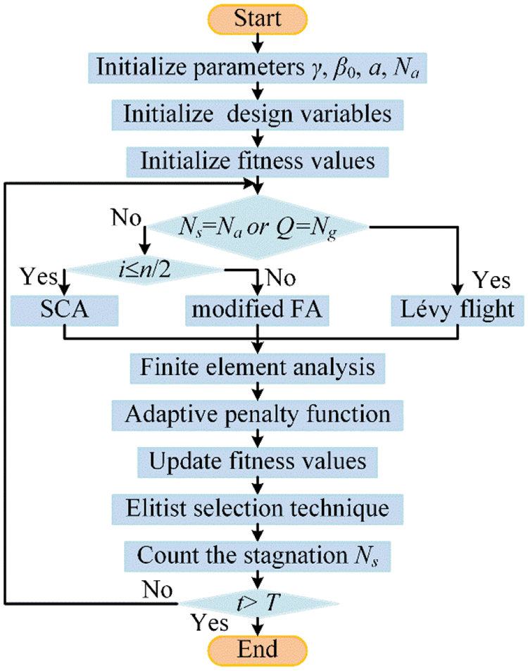
Figure 5: The flowchart of HSCFA

As shown in Fig. 5, the steps of the proposed algorithm are given in details as follows:

Step 1. Initialize the parameters γ, β0, a, Na.

Step 2. Initial solutions and the fitness values.

Step 3. If Q = Ng or Ns = Na, the solutions update by Eq (13). Otherwise, the population is divided into two equivalent parts that used modified FA and SCA for solution update. For i∈(1,n/2), every solution is updated by Eq. (5). For i∈(n/2+1,n), every solution is updated by Eq. (18).

Step 4. The finite element analysis is applied.

Step 5. The results obtained by finite element analysis are treated by the adaptive penalty function method. Count the number of stagnations Ns per solution.

Step 6. Use the elitist selection technique to select the solution.

Step 7. If the terminal condition is satisfied, end the iteration. Otherwise, it goes to Step 3.

5  Experiments and Results

In this section, the initial parameters of HSCFA are investigated and four well-known structural design problems including two size optimization and two shape and size optimization examples are tested. These structural design examples are all minimization problems with frequency constraints [32–34]. The optimization results of HSCFA are compared with SCA, FA and results of other methods in the existing researches. Different population sizes and iteration times are assigned to different experiments. Every experiment runs 20 times for SCA, FA, modified FA (MFA), HSCFA without Levy-flight and self-adaptivity of penalty function (HSCFA-1), HSCFA without self-adaptivity of penalty function (HSCFA-2) and HSCFA.

5.1 Investigation of Initial Parameters

Since the performance of HSCFA is influenced by β0, a and Na, different initial parameters are tested by the benchmark functions in Table 1. The dimension of the problems is set to 10. The population size and the iteration time are 20 and 100, and HSCFA runs 20 times for all the cases. For convenience, some of the results are illustrated in Figs. 6 and 7.

Figure 6: The changes of Fmean with β0

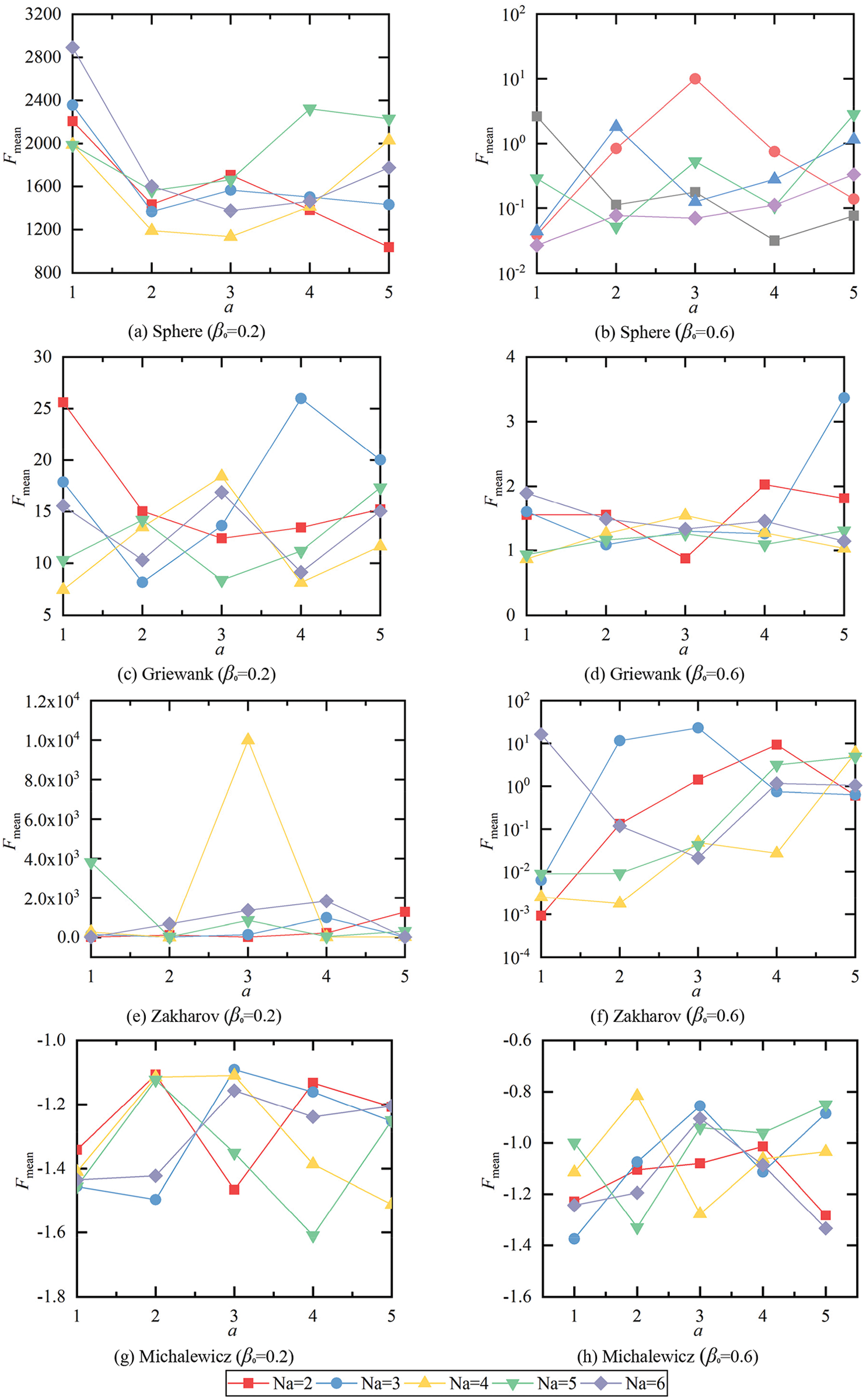
Figure 7: The changes of Fmean with a

From Fig. 6, the values of Fmean decrease with the increase of β0 for all the functions except for Michalewicz function. It is difficult to determine which value of β0 is the most reasonable one for Michalewicz function. From Fig. 7, the values of Fmean change irregularly with the increase of a. The relationship between the values of Fmean and Ns are also hard to be summarized from Figs. 6 and 7. Therefore, the Friedman and Wilcoxon tests are implemented to provide a more accurate evaluation of the initial parameters. The results are listed in Tables 2–9. The results of Wilcoxon tests below 0.05 denote the performance is much better than others.

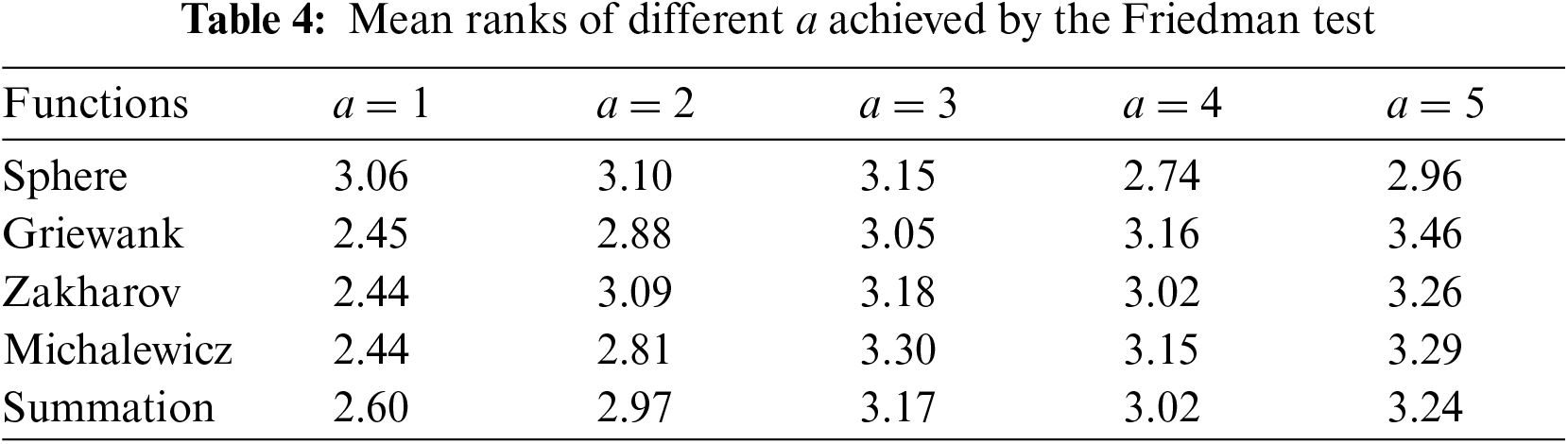
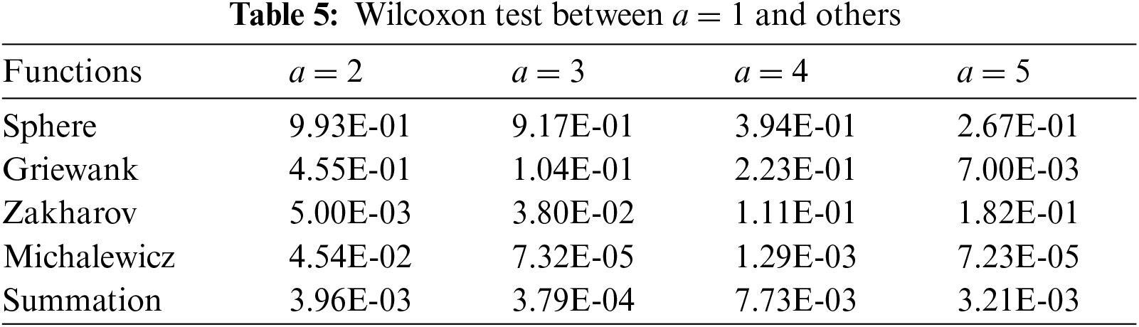
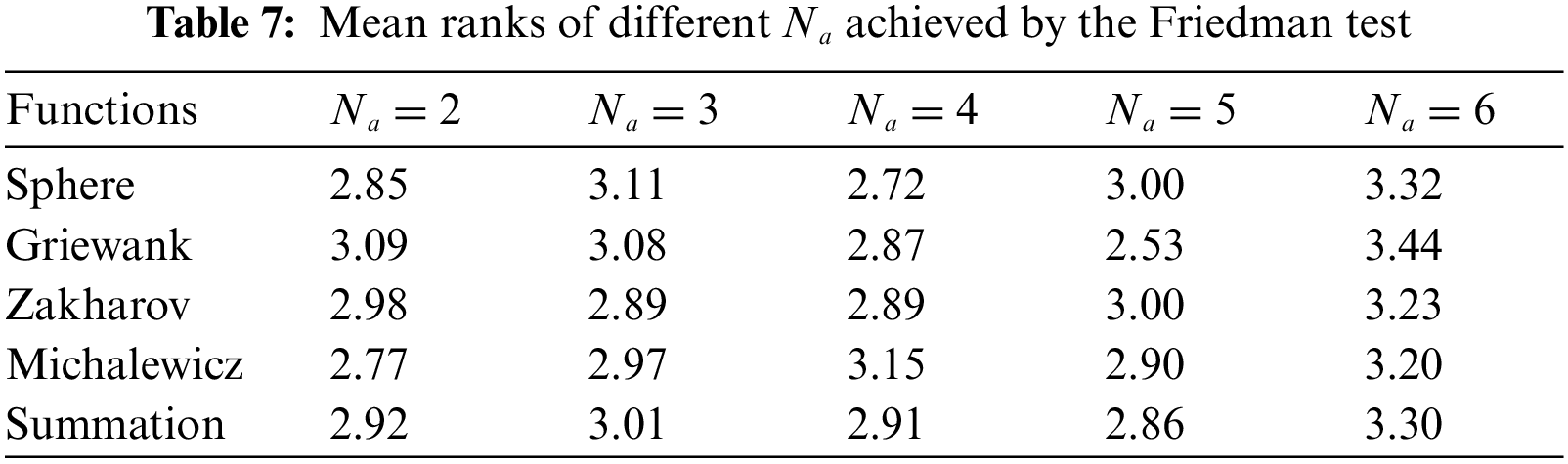
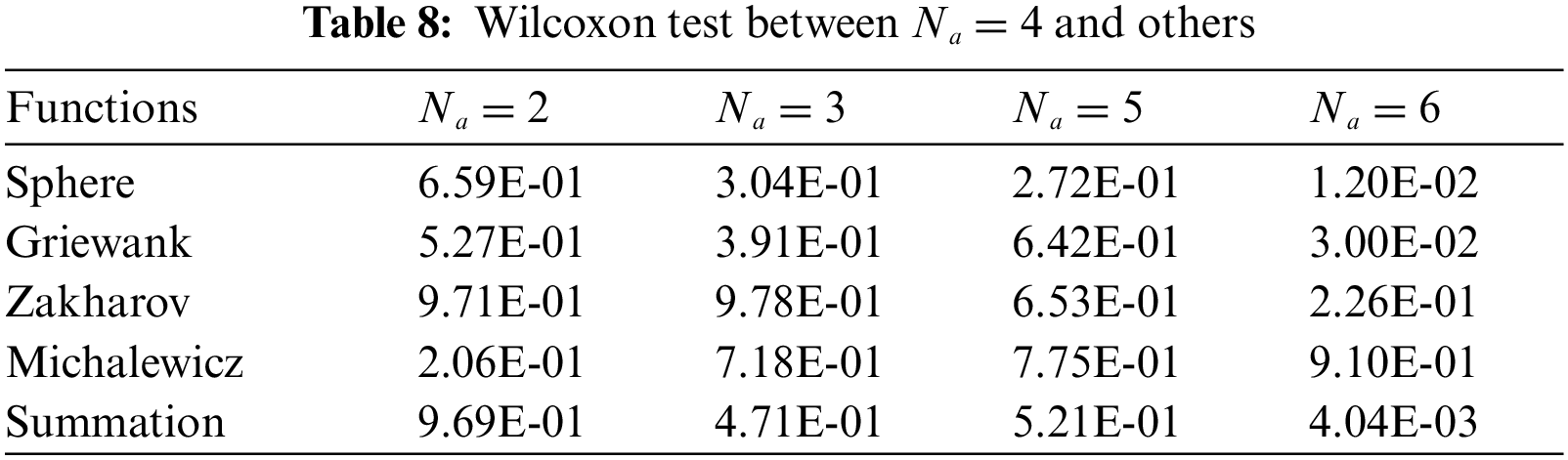
From Table 2, HSCFA performs best for Sphere, Griewank, and Zakharov functions when β0 = 1. Furthermore, it can be concluded from Table 3 that the algorithm performance is significantly better than others when β0 = 1. From Table 4, a = 1 ranks first for three functions and a = 4 ranks first for one function. From Tables 5 and 6, when a = 1, the results are significantly better than the other values for most of the cases. From Table 7, the rankings are different for each function and Na = 5 ranks first in Summation. From Tables 8 and 9, Na = 4 and Na = 5 are better than Na = 6 for two functions. Based on the Friedman and Wilcoxon tests, β0 = 1, a = 1 and Na = 5 are the proper initial parameters corresponding to the optimal performance of HSCFA.

5.2 Size Optimization

5.2.1 72-Bar Space Truss Structure

The 72-bar space truss including 16 size design variables is adopted as the first example. The geometry and support conditions are shown in Fig. 8. As shown in Fig. 8, four additional mass are located at nodes 1–4. Table 10 summarizes the design parameters and the frequency constraints. The results of PSO [35], harmony search (HS) [36], particle swarm ray optimization (PSRO) [37], harmony search-based mechanism to PSO with an aging leader and challengers (HALC-PSO) [38], cyclical parthenogenesis algorithm (CPA) [6], SCA and FA are used for the comparison. Table 11 displays the comparison of the results, where “Best” and “Mean” are the best and mean results, “NS” is the number of analyses, and “SD” is the standard deviation of results. Table 12 presents the first five natural frequencies of the optimal results. Fig. 9 shows the convergence histories of the best result of SCA, FA and HSCFA.

Figure 8: A 72-bar space truss structure

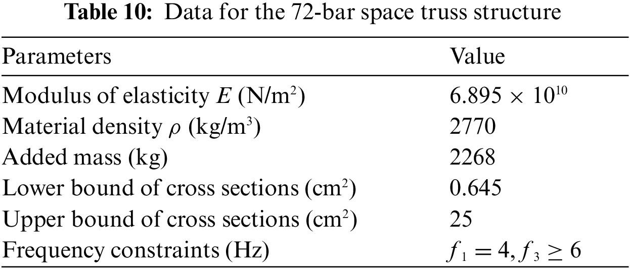
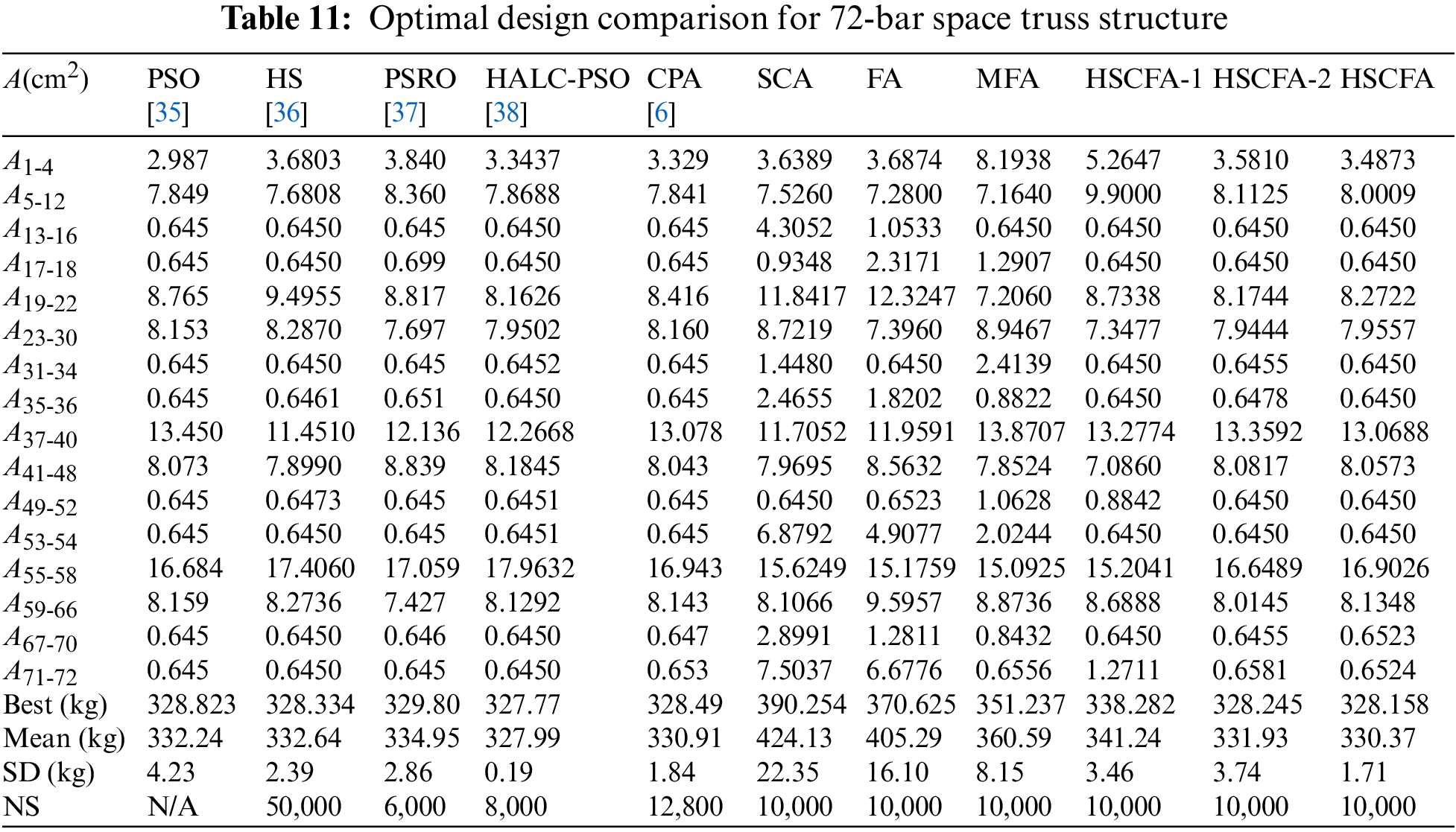
Figure 9: Iteration histories of 72-bar planar truss structure

For this experiment, the population size is 10 and the iteration is 1000 for SCA, FA, MFA, HSCFA-1, HSCFA-2, and HSCFA. Table 11 shows that HSCFA ranks second. However, the natural frequencies of HALC-PSO are 3.9985, 3.9985, 5.9985, 6.2285 and 9.0377, which violate the frequency constraints. HSCFA achieves a significant improvement compared to SCA and FA, and HSCFA makes at least 11.46% reduction in structural weight. It also can be found that the modification of FA and the hybrid technique improve the solution accuracy of the algorithm by comparing FA, MFA and HSCFA-1. The Lévy flight and self-adaptive penalty function can enhance the robust of the algorithm through the comparison of HSCFA-1, HSCFA-2 and HSCFA. Table 12 denotes the results of HSCFA satisfy the frequency constraints. Fig. 9 shows HSCFA has a faster convergence rate than SCA and FA. It is worth mentioning that the solution of HSCFA still gains improvement at the later iterations, which means the algorithm still has the ability to jump out of the local optimal.

5.2.2 120-Bar Dome Truss Structure

The 120-bar dome truss including 7 size design variables is adopted as the second example. The geometry and support conditions are shown in Fig. 10. Constant concentrated masses are added to Node 1, Nodes 2–13, and the rest of all free nodes, respectively. Table 13 summarizes the design parameters and the frequency constraints. The results of PSRO [37], PSO [38], HALC-PSO [38], set theoretical multi-phase teaching-learning-based optimization (STMP-TLBO) [39], enhanced forensic-based investigation algorithm (EFBI) [40], SCA and FA are used for the comparison. Table 14 lists the comparison of the results, and Table 15 presents the first five natural frequencies of the optimal results. Fig. 11 shows the convergence histories of the best result of SCA, FA and HSCFA.

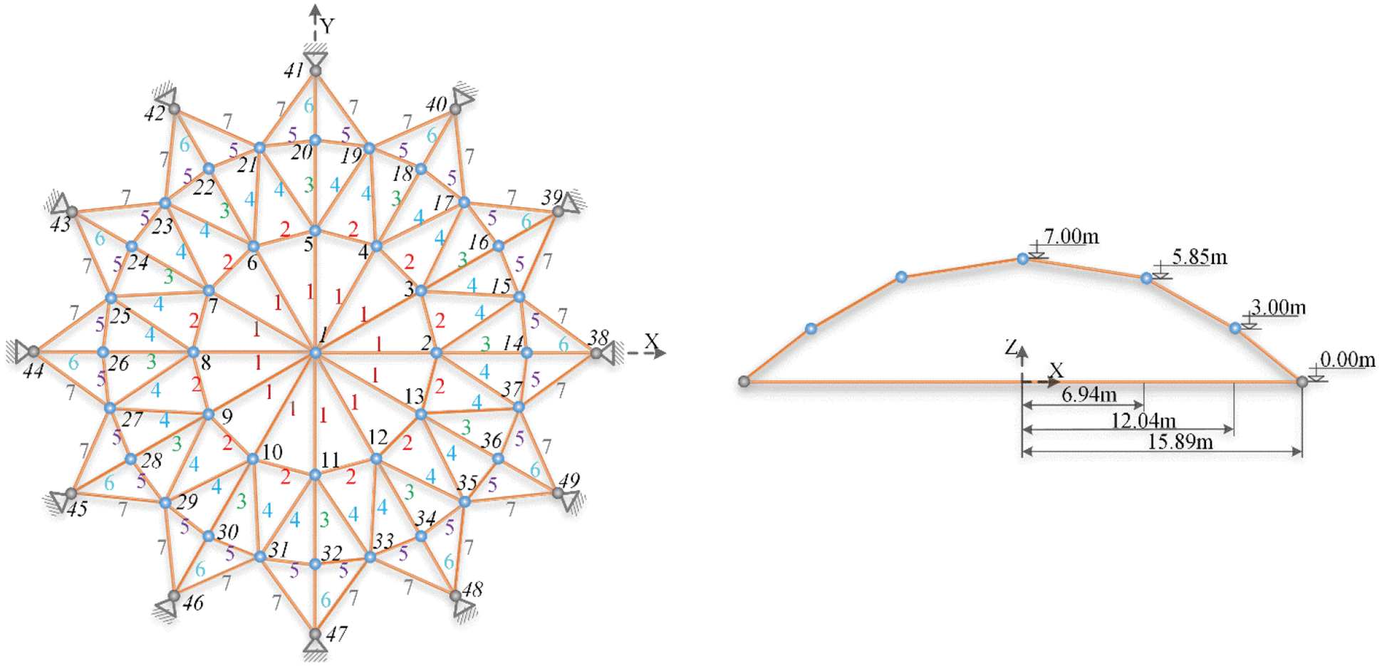
Figure 10: A 120-bar dome truss structure

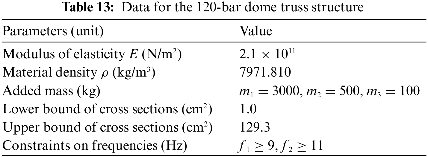
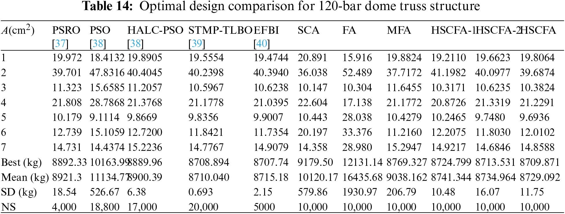
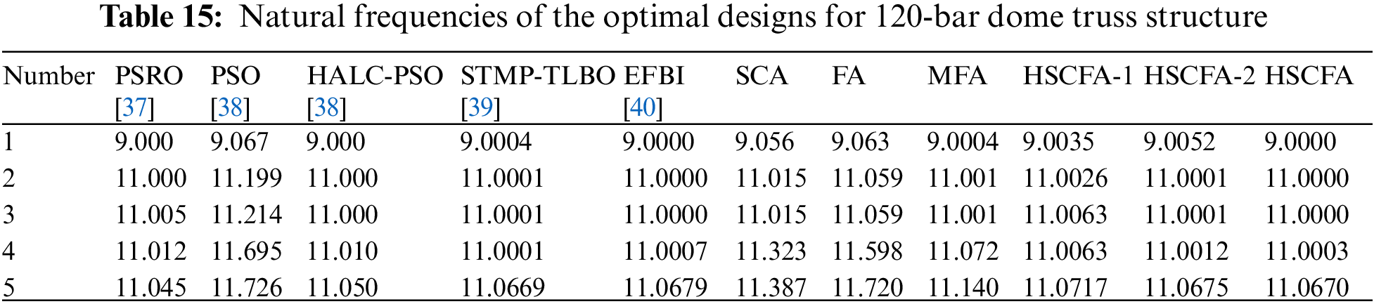
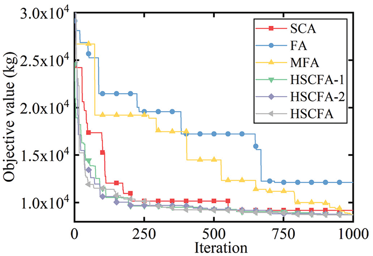
Figure 11: Iteration histories of 120-bar dome truss structure

For this experiment, the population size is 10 and the iteration is 1000 for SCA, FA, MFA, HSCFA-1, HSCFA-2, and HSCFA. Table 14 shows that HSCFA gains 5.12% and 28.20% loss of weight compared to the two original algorithms. The comparison of SCA, FA, MFA, HSCFA-1, HSCFA-2 and HSCFA denotes that the proposed strategies can improve the solution accuracy and robust. Table 15 indicates the adaptive penalty function can handle the frequency constraints well. Fig. 11 shows that SCA, HSCFA-1, HSCFA-2 and HSCFA have fast convergence rate at the early iterations. However, SCA has the problem of update stagnation at the later iterations. The solutions of HSCFA-1, HSCFA-2 and HSCFA update iteratively until the termination.

5.3 Shape and Size Optimization

5.3.1 37-Bar Planar Truss Structure

The 37-bar planar truss including 5 shape and 14 size design variables is used as the third example. The geometry and support conditions are shown in Fig. 12. Table 16 lists the design parameters and the allowable multiple natural frequency constraints. All the members in the lower chord have a constant cross-sectional area 40 cm2, and all the nodes in the lower chord attach a constant concentrated mass 10 kg. All nodes of the upper chord can vary from 1 m to 2.5 m in the y-axis. The results of NHPGA [41], HS [36], DPSO [5], PSRO [37], HALC-PSO [38], CPA [6], STMP-TLBO [39], SCA and FA are used for the comparison. Table 17 lists the comparison of optimal results, where “N/A” means the value is not available in the relative literature. Table 18 shows the first five natural frequencies of the optimal results. Fig. 13 illustrates the convergence histories of the best result of SCA, FA and HSCFA.

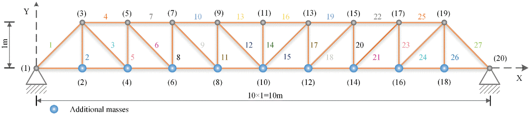
Figure 12: A 37-bar planar truss structure

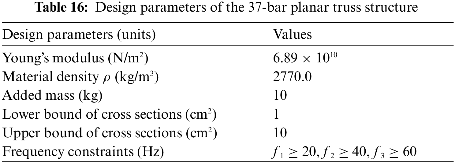
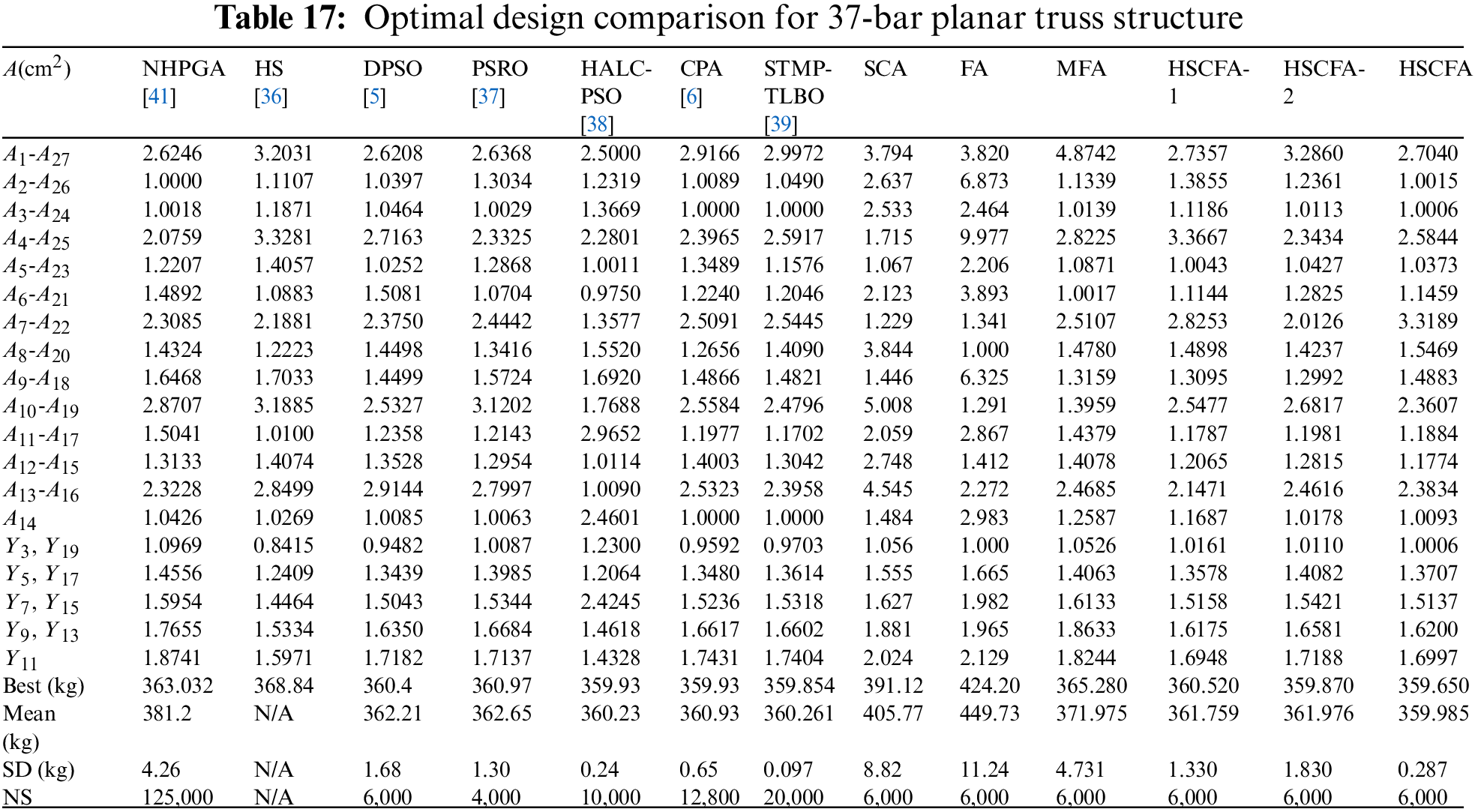
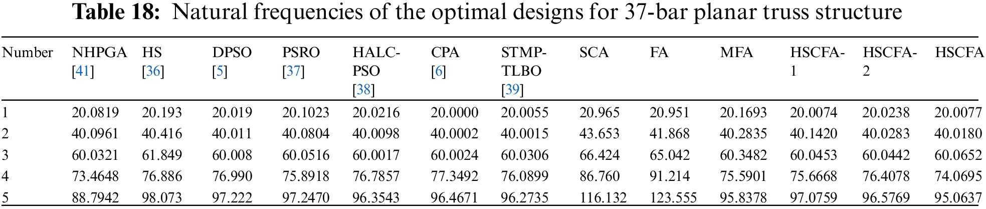
Figure 13: Iteration histories of 37-bar planar truss structure

For this experiment, the population size is 10 and the iteration is 600 for SCA, FA, MFA, HSCFA-1, HSCFA-2, and HSCFA. It can be concluded from Table 17 that HSCFA and STMP-TLBO rank first and second, but HSCFA obtains the lightest design with less analyses compared to CPA. Compare to SCA, FA, MFA, HSCFA-1 and HSCFA-2, the values of “Best”, “Mean” and “SD” indicate that HSCFA makes a great improvement in the solution accuracy and robustness. Table 18 shows the results of HSCFA satisfying the frequency constraints. Fig. 13 illustrates that HSCFA has the fastest convergence rate among the algorithms.

5.3.2 52-Bar Dome Truss Structure

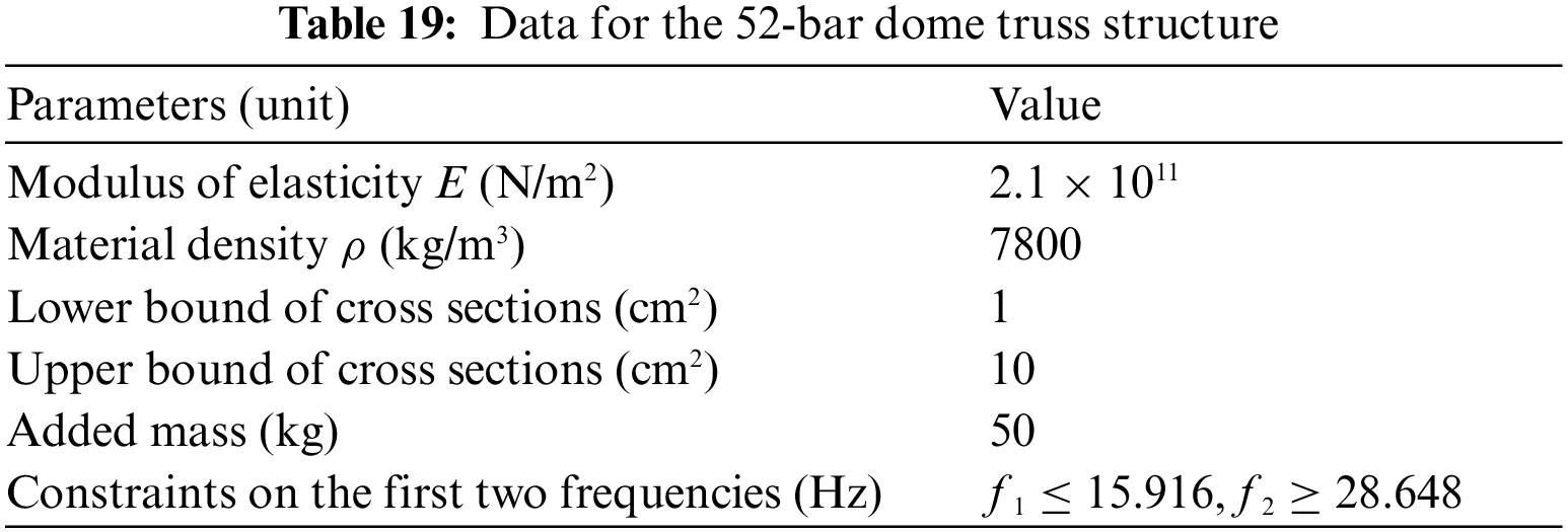
The 52-bar dome truss including 8 size and 5 shape design variables is adopted as the fourth example. The geometry and support conditions are shown in Fig. 14. Table 19 summarizes the design parameters and the allowable frequency constraints. All free nodes are permitted to move ±2 m in each allowable direction from their initial position on the basis of ensuring the symmetry of the whole structure. And constant concentrated mass is added to each free node. The results of NHPGA [41], HS [36], DPSO [5], PSRO [37], HALC-PSO [38], CPA [6], STMP-TLBO [39], EFBI [40], SCA and FA are used for the comparison. Comparison of the results and the first five frequency of best results for all the algorithms are reported in Tables 20 and 21. Fig. 15 shows the convergence histories of the best result of SCA, FA and HSCFA.

Figure 14: A 52-bar dome truss structure

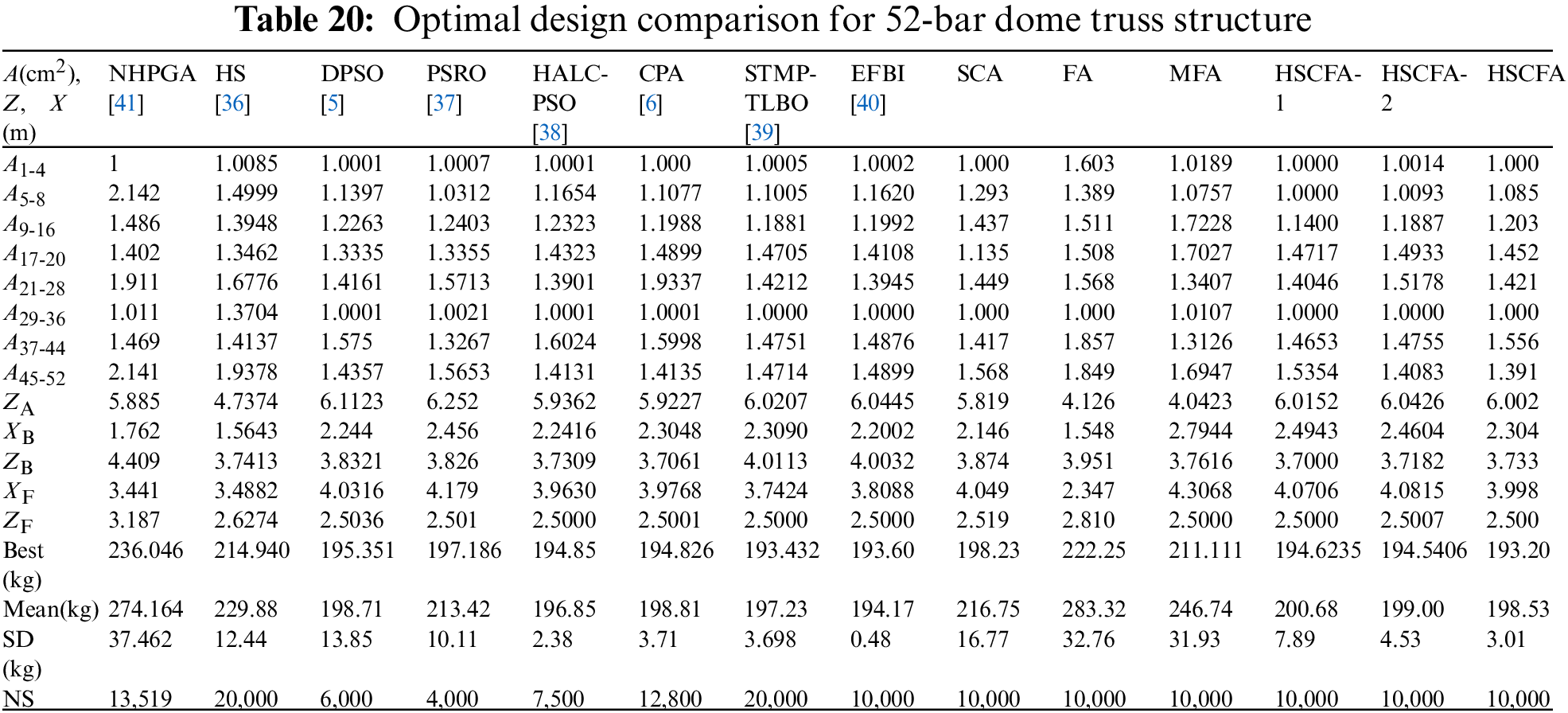
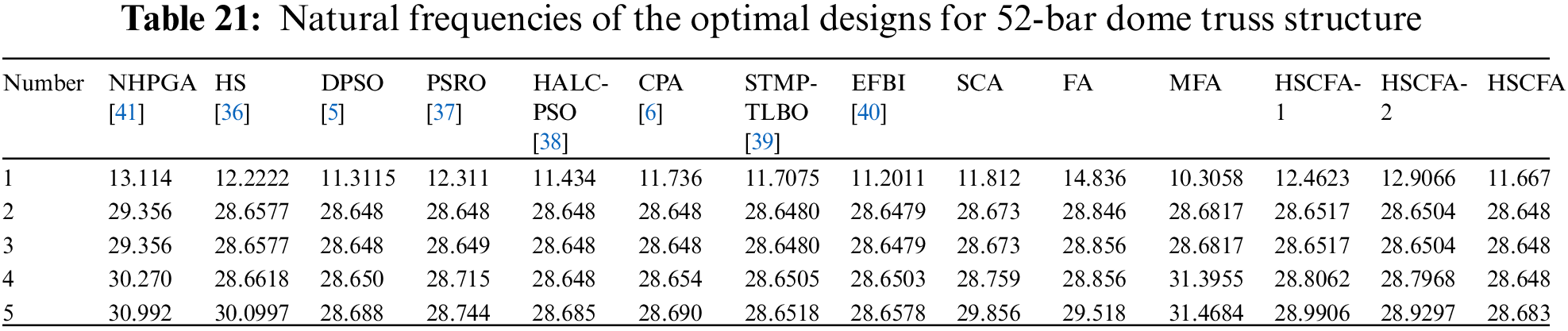
For this experiment, the population size is 10 and the iteration is 1000 for SCA, FA, MFA, HSCFA-1, HSCFA-2, and HSCFA. Table 20 shows that the best solution is acquired by HSCFA. The comparison of SCA, FA, MFA, HSCFA-1, HSCFA-2 and HSCFA indicates that the improvements can successfully enhance the performance of the algorithm. Table 21 shows the design of HSCFA satisfies the frequency constraints. It can be seen from Fig. 15 that HSCFA has a faster convergence rate than SCA and FA through the entire search process.

Figure 15: Iteration histories of 52-bar dome truss structure

6  Conclusions

A new hybrid metaheuristic method HSCFA is proposed to address the shape and size optimization of truss structures with nonstructural masses under multiple frequency constraints. The modified FA, SCA, Lévy flight, elitist selection technique and adaptive penalty function are integrated to construct the new method. The modified FA improves the attraction model of the standard FA by reducing the attraction number of each firefly, thus the solution accuracy is improved. The modified FA also uses the parameter of SCA instead of the original randomization parameter, which strengthens the exploitation ability of the algorithm. Lévy flight is utilized to improve the population diversity of the algorithm during the search process. Elitist selection technique is introduced into HSCFA for population selection to accelerate the convergence rate. An adaptive penalty function method considering the iteration stage, the degree and the number of constraint violations is adopted to deal with the frequency constraints. HSCFA takes advantage of the modified FA, SCA and Lévy flight to update different solutions. The modification enhances the exploration and exploitation abilities of FA and SCA with the reduction of computational complexity.

Four shape and size truss optimization problems with multiple frequency constraints are used to test the performance of HSCFA. The results demonstrate HSCFA performs better than other algorithms in the literature and achieves significant improvement compared to SCA and FA. HSCFA can obtain the lightest designs and cost the least computational time. Consequently, HSCFA provides an efficient and competitive tool for shape and size optimization problems with frequency constraints.

Funding Statement: This work is supported by the National Natural Science Foundation of China (No. 11672098).

Conflicts of Interest: The authors declare that they have no conflicts of interest to report regarding the present study.

References

1. Bellagamba, L., Yang, T. Y. (1981). Minimum-mass truss structures with constraints on fundamental natural frequency. AIAA Journal, 19(11), 1452–1458. DOI 10.2514/3.7875. [Google Scholar] [CrossRef]
2. Grandhi, R. V., Venkayya, V. B. (1988). Structural optimization with frequency constraints. AIAA Journal, 26(7), 858–866. DOI 10.2514/3.9979. [Google Scholar] [CrossRef]
3. Wei, L., Zhao, M., Wu, G., Meng, G. (2005). Truss optimization on shape and sizing with frequency constraints based on genetic algorithm. Computational Mechanics, 35(5), 361–368. DOI 10.1007/s00466-004-0623-8. [Google Scholar] [CrossRef]
4. Ho-Huu, V., Nguyen-Thoi, T., Truong-Khac, T., Le-Anh, L., Vo-Duy, T. (2018). An improved differential evolution based on roulette wheel selection for shape and size optimization of truss structures with frequency constraints. Neural Computing and Applications, 29(1), 167–185. DOI 10.1007/s00521-016-2426-1. [Google Scholar] [CrossRef]
5. Kaveh, A., Zolghadr, A. (2014). Democratic PSO for truss layout and size optimization with frequency constraints. Computers & Structures, 130(12), 10–21. DOI 10.1016/j.compstruc.2013.09.002. [Google Scholar] [CrossRef]
6. Kaveh, A., Zolghadr, A. (2017). Cyclical parthenogenesis algorithm for layout optimization of truss structures with frequency constraints. Engineering Optimization, 49(8), 1317–1334. DOI 10.1080/0305215X.2016.1245730. [Google Scholar] [CrossRef]
7. Lieu, Q. X., Do, D. T. T., Lee, J. (2018). An adaptive hybrid evolutionary firefly algorithm for shape and size optimization of truss structures with frequency constraints. Computers and Structures, 195, 99–112. DOI 10.1016/j.compstruc.2017.06.016. [Google Scholar] [CrossRef]
8. Yang, X. S. (2010). Firefly algorithm, stochastic test functions and design optimisation. International Journal of Bio-Inspired Computation, 2(2), 78–84. DOI 10.1504/IJBIC.2010.032124. [Google Scholar] [CrossRef]
9. Yang, X. S. (2014). Nature-inspired algorithms and applied optimization. Oxford: Elsevier. [Google Scholar]
10. Gandomi, A. H., Yang, X. S., Alavi, A. H. (2011). Mixed variable structural optimization using firefly algorithm. Computers and Structures, 89(23-24), 2325–2336. DOI 10.1016/j.compstruc.2011.08.002. [Google Scholar] [CrossRef]
11. Erdal, F. (2017). A firefly algorithm for optimum design of new-generation beams. Engineering Optimization, 49(6), 915–931. DOI 10.1080/0305215X.2016.1218003. [Google Scholar] [CrossRef]
12. Tao, R., Meng, Z., Zhou, H. L. (2021). A self-adaptive strategy based firefly algorithm for constrained engineering design problems. Applied Soft Computing, 107(1), 107417. DOI 10.1016/j.asoc.2021.107417. [Google Scholar] [CrossRef]
13. Goel, R., Maini, R. (2018). A hybrid of ant colony and firefly algorithms (HAFA) for solving vehicle routing problems. Journal of Computational Science, 25(1), 28–37. DOI 10.1016/j.jocs.2017.12.012. [Google Scholar] [CrossRef]
14. Pitchaimanickam, B., Murugaboopathi, G. (2020). A hybrid firefly algorithm with particle swarm optimization for energy efficient optimal cluster head selection in wireless sensor networks. Neural Computing and Applications, 32(12), 7709–7723. DOI 10.1007/s00521-019-04441-0. [Google Scholar] [CrossRef]
15. Lieu, Q. X., Do, D. T. T., Lee, J. (2018). An adaptive hybrid evolutionary firefly algorithm for shape and size optimization of truss structures with frequency constraints. Computers & Structures, 195, 99–112. DOI 10.1016/j.compstruc.2017.06.016. [Google Scholar] [CrossRef]
16. Chou, J. S., Ngo, N. T. (2017). Modified firefly algorithm for multidimensional optimization in structural design problems. Structural and Multidisciplinary Optimization, 55(6), 2013–2028. DOI 10.1007/s00158-016-1624-x. [Google Scholar] [CrossRef]
17. Mirjalili, S. (2016). SCA: A sine cosine algorithm for solving optimization problems. Knowledge-Based Systems, 96(63), 120–133. DOI 10.1016/j.knosys.2015.12.022. [Google Scholar] [CrossRef]
18. Li, S., Fang, H. J., Liu, X. Y. (2018). Parameter optimization of support vector regression based on sine cosine algorithm. Expert Systems with Applications, 91(11), 63–77. DOI 10.1016/j.eswa.2017.08.038. [Google Scholar] [CrossRef]
19. Yıldız, B., Yıldız, A. (2018). Comparison of grey wolf, whale, water cycle, ant lion and sine-cosine algorithms for the optimization of a vehicle engine connecting rod. Materials Testing, 60(3), 311–315. DOI 10.3139/120.111153. [Google Scholar] [CrossRef]
20. Mahdad, B., Srairi, K. (2018). A new interactive sine cosine algorithm for loading margin stability improvement under contingency. Electrical Engineering, 100(2), 913–933. DOI 10.1007/s00202-017-0539-x. [Google Scholar] [CrossRef]
21. Bhadoria, A., Marwaha, S., Kamboj, V. K. (2020). An optimum forceful generation scheduling and unit commitment of thermal power system using sine cosine algorithm. Neural Computing and Applications, 32(7), 2785–2814. DOI 10.1007/s00521-019-04598-8. [Google Scholar] [CrossRef]
22. Yang, X. S. (2018). Nature-inspired algorithms and applied optimization. London: Springer. [Google Scholar]
23. Chechkin, A. V., Metzler, R., Klafter, J., Gonchar, V. Y. (2008). Introduction to the theory of Lévy flights. Anomalous Transport. Germany: Wiley‐VCH Verlag GmbH & Co. KGaA. [Google Scholar]
24. Chegini, S. N., Bagheri, A., Najafi, F. (2018). PSOSCALF: A new hybrid PSO based on sine cosine algorithm and Levy flight for solving optimization problems. Applied Soft Computing, 73(3), 697–726. DOI 10.1016/j.asoc.2018.09.019. [Google Scholar] [CrossRef]
25. Haklı, H., Uğuz, H. (2014). A novel particle swarm optimization algorithm with Levy flight. Applied Soft Computing, 23(3), 333–345. DOI 10.1016/j.asoc.2014.06.034. [Google Scholar] [CrossRef]
26. Yang, X. S. (2010). Engineering optimization: An introduction with metaheuristic applications. USA: John Wiley & Sons. [Google Scholar]
27. Padhye, N., Bhardawaj, P., Deb, K. (2013). Improving differential evolution through a unified approach. Journal of Global Optimization, 55(4), 771–799. DOI 10.1007/s10898-012-9897-0. [Google Scholar] [CrossRef]
28. John, R. M., Robert, G. R., David, B. F. (1995). A survey of constraint handling techniques in evolutionary computation methods. Evolutionary Programming IV: Proceedings of the Fourth Annual Conference on Evolutionary Programming, pp. 135–155. San Diego, California, USA. [Google Scholar]
29. Coello, C. A. C. (2002). Theoretical and numerical constraint-handling techniques used with evolutionary algorithms: A survey of the state of the art. Computer Methods in Applied Mechanics and Engineering, 191(11), 1245–1287. DOI 10.1016/S0045-7825(01)00323-1. [Google Scholar] [CrossRef]
30. Wang, H., Wang, W. J., Sun, H., Rahnamayan, S. (2016). Firefly algorithm with random attraction. International Journal of Bio-Inspired Computation, 8(1), 33–41. DOI 10.1504/IJBIC.2016.074630. [Google Scholar] [CrossRef]
31. Wang, H., Wang, W. J., Zhou, X. Y., Sun, H., Zhao, J. et al. (2017). Firefly algorithm with neighborhood attraction. Information Sciences, 382--383(7), 374–387. DOI 10.1016/j.ins.2016.12.024. [Google Scholar] [CrossRef]
32. Li, L. J., Huang, Z. B., Liu, F. (2009). A heuristic particle swarm optimization method for truss structures with discrete variables. Computers & Structures, 87(7--8), 435–443. DOI 10.1016/j.compstruc.2009.01.004. [Google Scholar] [CrossRef]
33. Cheng, M. Y., Prayogo, D., Wu, Y. W., Lukito, M. M. (2016). A hybrid harmony search algorithm for discrete sizing optimization of truss structure. Automation in Construction, 69(7), 21–33. DOI 10.1016/j.autcon.2016.05.023. [Google Scholar] [CrossRef]
34. Shahabsafa, M., Mohammad-Nezhad, A., Terlaky, T., Zuluaga, L., He, S. et al. (2018). A novel approach to discrete truss design problems using mixed integer neighborhood search. Structural and Multidisciplinary Optimization, 58(6), 2411–2429. DOI 10.1007/s00158-018-2099-8. [Google Scholar] [CrossRef]
35. Gomes, H. M. (2011). Truss optimization with dynamic constraints using a particle swarm algorithm. Expert Systems with Applications, 38(1), 957–968. DOI 10.1016/j.eswa.2010.07.086. [Google Scholar] [CrossRef]
36. Miguel, L. F. F., Miguel, L. F. F. (2012). Shape and size optimization of truss structures considering dynamic constraints through modern metaheuristic algorithms. Expert Systems with Applications, 39(10), 9458–9467. DOI 10.1016/j.eswa.2012.02.113. [Google Scholar] [CrossRef]
37. Kaveh, A., Zolghadr, A. (2014). A new PSRO algorithm for frequency constraint truss shape and size optimization. Structural Engineering and Mechanics, 52(3), 445–468. DOI 10.12989/sem.2014.52.3.445. [Google Scholar] [CrossRef]
38. Kaveh, A., Ghazaan, M. I. (2015). Hybridized optimization algorithms for design of trusses with multiple natural frequency constraints. Advances in Engineering Software, 79(12), 137–147. DOI 10.1016/j.advengsoft.2014.10.001. [Google Scholar] [CrossRef]
39. Kaveh, A., Hamedani, K. B., Kamalinejad, M. (2020). Set theoretical variants of the teaching-learning-based optimization algorithm for optimal design of truss structures with multiple frequency constraints. Acta Mechanica, 231(9), 3645–3672. DOI 10.1007/s00707-020-02718-3. [Google Scholar] [CrossRef]
40. Kaveh, A., Hamedani, K. B., Kamalinejad, M. (2021). An enhanced forensic-based investigation algorithm and its application to optimal design of frequency-constrained dome structures. Computers & Structures, 256(24), 106643. DOI 10.1016/j.compstruc.2021.106643. [Google Scholar] [CrossRef]
41. Wei, L., Tang, T., Xie, X., Shen, W. (2011). Truss optimization on shape and sizing with frequency constraints based on parallel genetic algorithm. Structural and Multidisciplinary Optimization, 43(5), 665–682. DOI 10.1007/s00158-010-0600-0. [Google Scholar] [CrossRef]
Cite This Article
Copyright © 2023 The Author(s). Published by Tech Science Press.
This work is licensed under a Creative Commons Attribution 4.0 International License , which permits unrestricted use, distribution, and reproduction in any medium, provided the original work is properly cited.
Downloads
Citation Tools