
 Submit a Paper
 Propose a Special lssue
 Open Access
ARTICLE
Stability Analysis of Landfills Contained by Retaining Walls Using Continuous Stress Method
1 China Academy of Railway Sciences Corporation Limited, Beijing, 100081, China
2 School of Civil, Architecture and Environment, Hubei University of Technology, Wuhan, 430068, China
* Corresponding Author: Yingfa Lu. Email:
(This article belongs to the Special Issue: Computational Mechanics Assisted Modern Urban Planning and Infrastructure)
Computer Modeling in Engineering & Sciences 2023, 134(1), 357-381. https://doi.org/10.32604/cmes.2022.020874
Received 16 December 2021; Accepted 07 March 2022; Issue published 24 August 2022
 View Full Text
 Download PDF
Abstract
An analytical method for determining the stresses and deformations of landfills contained by retaining walls is proposed in this paper. In the proposed method, the sliding resisting normal and tangential stresses of the retaining wall and the stress field of the sliding body are obtained considering the differential stress equilibrium equations, boundary conditions, and macroscopic forces and moments applied to the system, assuming continuous stresses at the interface between the sliding body and the retaining wall. The solutions to determine stresses and deformations of landfills contained by retaining walls are obtained using the Duncan-Chang and Hooke constitutive models. A case study of a landfill in the Hubei Province in China is used to validate the proposed method. The theoretical stress results for a slope with a retaining wall are compared with FEM results, and the proposed theoretical method is found appropriate for calculating the stress field of a slope with a retaining wall.Keywords
Retaining walls are typically used to support subgrade or sloped fills, stabilize embankments, and prevent deformation failures, or reduce the height of sloped excavations. In order to mitigate the failure risk of a sliding slope supported by a retaining wall, an effective protection solution must be employed to ensure the stability of the slope [1]. The calculation of the active earth pressure behind a retaining wall is a classical problem in soil mechanics. The conventional design methods of retaining walls usually require estimating the earth pressure behind a wall and selecting a wall geometry to satisfy the equilibrium conditions with a specified factor of safety. Closed-form solutions are widely used for computing the active earth thrust acting on retaining structures in the equilibrium limit state. However, the active earth pressure calculation methods still have many issues, such as determining the resultant force line of action. Since the deformation failure mode of a retaining wall cannot be accurately predicted, a sliding surface is assumed to simplify the calculations. Du Bois [2] proposed the active and passive earth pressure coefficients and equations for calculating the lateral earth pressure acting on retaining walls in the equilibrium limit state. The Coulomb earth pressure theory assumes a planar sliding surface for a cohesionless wall and a triangular earth pressure distribution. The Rankine earth pressure theory is based on a semi-infinite space and assumes that the wall is rigid, the back of the wall is vertical and smooth, the surface of fill behind the wall is horizontal, and the distribution of earth pressure is triangular. The Rankine theory can be used directly to calculate the earth pressure for cohesive soils, but the results are very conservative. Okabe et al. [3,4] suggested a calculation method for the lateral earth thrust in seismic conditions. Terzaghi [5] suggested that the active earth pressure of the rigid retaining wall is related to the movement of the retaining wall. There are obvious differences in the active earth pressure of the rigid retaining walls under three different movement modes: translation, top rotation, and bottom rotation. Kezdi [6] studied the rotational movement modes of a retaining wall around its bottom. Handy [7] considered the soil arching effect to study the stress distribution in the soil mass behind the retaining wall using the finite element method and assuming a Rankine sliding surface. In actual engineering applications, the evaluation of the lateral earth thrust due to the soil weight and the surcharge acting on the retained backfill may be required. However, the available solutions for the active earth pressure acting on retaining walls are only suitable for static conditions. Motta [8] proposed a general closed-form solution for the case of uniformly distributed surcharge applied on the backfill soil at a certain distance from the top of the wall.
The slope failure mechanism and stability analysis are traditional topics in geotechnical engineering. Previous studies have proposed many equilibrium limit stability calculation methods, such as the Fellenius method, simplified Bishop method, Spencer method, Janbu method, transfer coefficient method, Sarma method, wedge method, and finite element strength reduction method (SRM) [9–16]. In the traditional slope stability analysis, the limit equilibrium slice method is often used [17–19]. With the advancement of numerical methods, various new calculation methods appeared [20–24], including the partial strength reduction methods (PSRM) that simulate the progressive failure of landslides [25,26]. The sliding surface is divided into an unstable zone, a critical zone, and a stable zone, and the characteristics of the critical stress state of the slope were proposed by [25–29]. However, limited studies adopting models of both the retaining wall and the slope have been carried out. Dawson et al. [30] established an analytical model for the retaining wall and the slope and analyzed the stability of a high-speed road slope using the limit equilibrium theory and the finite element method (FEM).
The current studies on slopes and retaining walls mainly focus on the earth pressure calculation and stability evaluation under some assumptions. Based on the classical theories of earth pressure, the sliding and overturning stability, and safety evaluation of retaining walls and slopes, a new method of force and displacement analysis of landfills contained with retaining walls is proposed in this article. The method has the following characteristics:
(1) A theoretical solution for the stress at any point of the landfill confined with a retaining wall can be obtained, considering the corresponding boundary conditions, but ignoring the critical state assumptions.
(2) The Duncan-Chang and Hooke constitutive models are used to obtain the strains and displacements in landfills confined with retaining walls.
(3) The proposed method can not only be used to study the overturning and sliding failure modes but the tensile and bulging failure modes of retaining walls and landfills as well. The overall internal failure evaluation of retaining walls and landfills can be carried out.
(4) The normal and tangential stresses produced by the lateral earth thrust acting on the retaining wall can be taken into account.
(5) The method provides a theoretical basis for slope design. Different retaining wall forms and materials can be adopted for different stress distributions, which can lead to economic, rational, and effective designs.
2 Traditional Retaining Wall Design
The conventional method for calculation of lateral stress for gravity retaining walls with rigid foundations and homogeneous cohesionless fills is introduced first.
2.1 Earth Pressure of Homogeneous Cohesionless Backfills
The active earth pressure acting on the retaining wall can be calculated for a homogeneous cohesionless backfill in Eq. (1).
where
When the backfill top surface behind the wall is inclined (see Fig. 1), the active earth pressure coefficient for a gravity retaining wall can be calculated in Eq. (2).
where
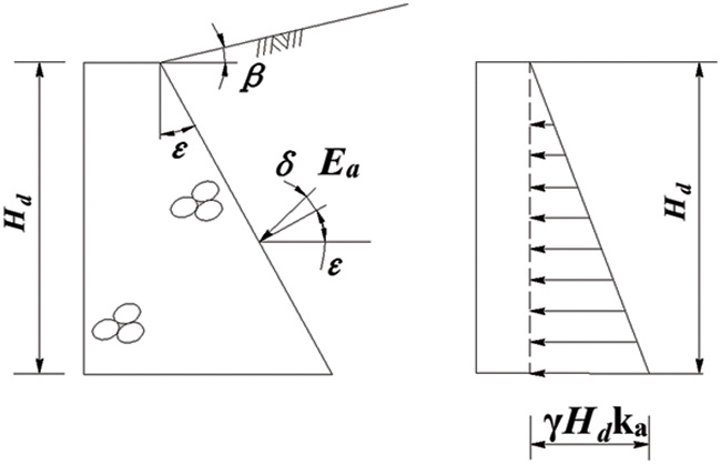
Figure 1: Gravity retaining wall with inclined infill top surface
2.2.1 Stress at Retaining Wall Base
The stress at the base of a retaining wall can be calculated in Eq. (3).
where
The stresses of the retaining wall founded on hard rock should meet the following criteria:
(1) The maximum retaining wall base stress should not be greater than the allowable bearing capacity of the hard rock; and
(2) Except for the construction period and under an earthquake excitation, there must be no tensile stress on the base of the retaining wall.
2.2.2 Base Sliding Stability of Retaining Wall
The safety factor against sliding of the retaining wall along the rock base is calculated according to Eq. (4).
where
When the retaining wall back surface is inclined towards the direction of the backfill, the safety factor along the surface between the retaining wall and rock can be calculated according to Eq. (5).
where
The factor of safety against overturning of a retaining wall is calculated according to Eq. (7).
where
According to the above formulas, the sliding stress is produced by the active earth pressure, and the resisting stresses include the compressive and shear strength at the wall base. However, the above results do not consider the tensile failure of the retaining wall. This paper presents a novel method of calculating the stresses and strains for a retaining wall.
3 New Landfill Analysis Method
When the shape of an object is determined, the stress solution must be clear and be updated with the boundary condition changes. Assuming the stresses are continuous, the solutions must satisfy the differential stress equilibrium equations and deformation boundary conditions. This method can be used to find the stress distribution for any geometry, including two-dimensional (2D) and three dimensional (3D) cases. When the boundary conditions and stress field are discontinuous, the discontinuous stress and displacement solutions can also be obtained. The landfill with a retaining wall is taken as an example to illustrate the basic ideas and approaches.
3.1 Boundary Conditions, Specific Gravity and Stresses
In this study, a theoretical solution for an arbitrary polygon under a 2D plane strain problem is studied. The landfill and the retaining wall are the polygon ABCDP and the quadrilateral element BCFE, respectively. The analysis steps are as follows:
(1) The boundaries of the analyzed system are assumed (see Fig. 2). A linear equation is used for the boundary segments AB, BC, CD, DP, and PA of the polygon ABCDP, and segments BE, EF, FC, and CB of the quadrilateral BCFE.
(2) The specific gravity (
(3) Using the stress field characteristics, the stress boundary conditions can be formed. The normal stresses at the transition between the landfill (i.e.,
where
(4) The landfill must satisfy the equilibrium equations, the stress boundary conditions, and the deformation equations. The expressions for the stress equilibrium equations are written and their coefficients are calculated. The stress expressions are assumed for a 2D landfill (note the stress expressions can be changed for different conditions) in Eqs. (10)–(12).
where
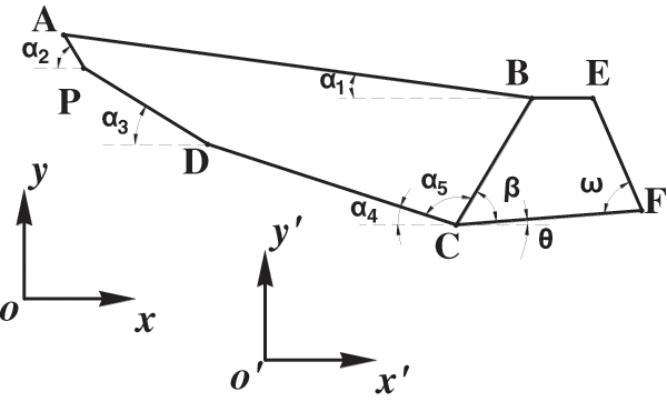
Figure 2: Sketch of landfill contained with retaining wall
The number of constant coefficients in Eqs. (10)–(12) can be reduced from 30 to 18 using the differential stress equilibrium equations, which depend on the boundary conditions and macro force equilibrium equations.
The following differential stress equilibrium equations, Eqs. (13) and (14), are satisfied at any point.
The corresponding coefficients are zero at any point with a constant unit weight (
3.2 Stress Relationships along Boundary Segment AB
Boundary segment AB of polygon ABCDP can be expressed mathematically in Eq. (15).
The stress conditions on boundary AB are in Eq. (16).
Eqs. (2-1)–(2-12) in Appendix were obtained using Eq. (16).
3.3 Force Equilibrium of Landfill
Once the landfill is in a balanced and stable state, the force equilibrium of polygon ABCDP in X- and Y-direction are in Eqs. (17) and (18).
where
The expressions for
3.3.1 Normal Forces Acting on Segments CD, BC, and PD
The equation of boundary segment CD is in Eq. (19)
The expressions for
By substituting Eqs. (20)–(22) into the normal stress equations one obtains Eq. (23).
where
The normal force acting on segment CD can be obtained by integration in Eq. (24).
The normal forces acting on segments BC and PD can be derived in a similar way. The equation for segment BC is in Eq. (25) and for PD is Eq. (26).
The resulting normal forces acting on segments BC and PD are in Eqs. (27) and (28), respectively.
3.3.2 Tangential Forces Acting on Segments CD and PD
The shear stresses between the landfill and the sliding bed are discontinuous. The frictional stresses along segment CD can be taken as the residual stress due to the sliding body with the landfill and expressed in Eq. (29).
where
By integrating Eq. (30), we obtain Eq. (31).
Simplifying Eqs. (30) and (31) yields Eq. (32).
The equation for segment PD is
3.3.3 Tangential Force Acting on Segment BC
The stresses between the landfill and the retaining wall are continuous. A similar method is adopted to calculate the shear stress along segment BC in Eq. (34), where
where
The weight (
as
The equation of boundary segment AP is in Eq. (37).
The shear stress resultant along segment AP can be assumed zero according to the Saint Venant principle shown in Eq. (38).
3.5 Coefficients for Landfill Solution
If coefficients
4 Theoretical Solution for Retaining Wall
The stresses acting on segments BC and CF of the retaining wall have been obtained. This section derives the stresses for the retaining wall assuming stress continuity between the landfill and the retaining wall. The coordinates used to analyze the retaining wall are shown Fig. 3.
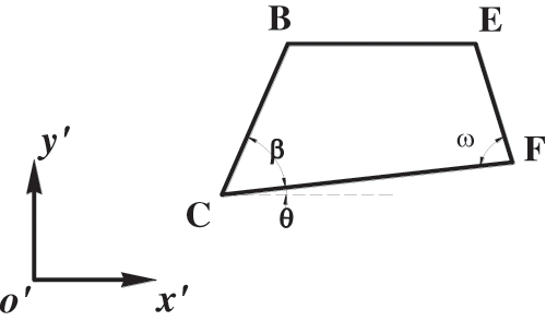
Figure 3: 2D model of retaining wall
4.1 Stress Continuity along Boundary Segment BC
Stress equilibrium is assumed along segments BC and CF based on the continuity of stresses between the landfill and the retaining wall and between the retaining wall and its base.
The equation for segment BC is Eq. (39).
In Eq. (40),
By combining Eqs. (39) and (40) with Eqs. (10)–(12), the normal and tangential stresses are calculated in Eqs. (41)–(43).
The stresses acting on the retaining wall are defined in the
where
Eq. (39) is substituted into Eq. (44) to yield Eq. (47).
Eqs. (3-1)–(3-4) in Appendix can be obtained assuming
4.2 Force Balance of Retaining Wall
The forces acting on the retaining wall include the normal and tangential forces along segment BC (
In Eqs. (48) and (49),
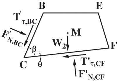
Figure 4: Force acting on retaining wall
The calculation statements are presented in the following form:
4.2.1 Normal Forces along Segments BC and CF
Eq. (50) for the retaining wall can be obtained using Eqs. (44)–(46).
where
The normal force acting on boundary segment BC of the retaining wall is obtained by integrating Eq. (51).
The normal stress on boundary segment CF is in Eq. (52).
In Eq. (53),
The normal force acting on boundary segment CF of the retaining wall is obtained by integrating Eq. (53), as shown in Eq. (54).
4.2.2 Tangential Forces along Segments BC and CF
A similar approach is adopted for calculating the tangential forces along segments BC and CF of the retaining wall in Eq. (55).
The tangential force acting on boundary segment BC can be achieved by integrating Eq. (55) in Eq. (56).
The shear stress acting on segment CF is in Eq. (57).
The tangential force acting on boundary segment CF is found by integrating Eq. (57) as shown in Eq. (58).
4.2.3 Weight and Barycentric Coordinate of Retaining Wall
The barycentric coordinates of triangles BEC and EFC are denoted as I and J, respectively. The barycentric coordinates (
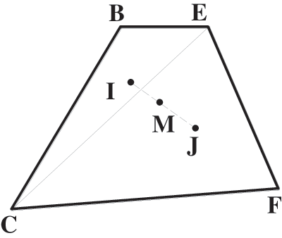
Figure 5: Retaining wall barycentric coordinate determination
The weight per unit thickness of the retaining wall is
4.3 Moment Balance of Retaining Wall
Point
Moments
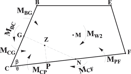
Figure 6: Moments acting on retaining wall
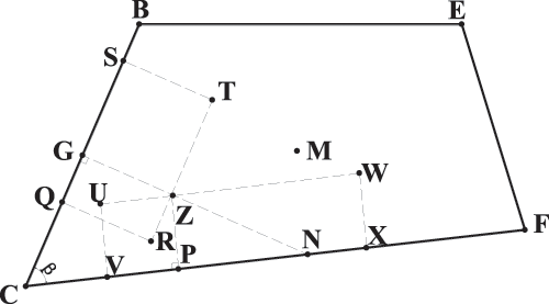
Figure 7: Lever arms of moment acting on retaining wall
The moment balance equation for the retaining wall can be written in Eq. (62).
The lever arms of moments
4.4 Free Point Stress Characteristics
The stresses at point E
Therefore, we have Eqs. (63)–(65).
4.5 Coefficients of Retaining Wall Solution
The 18 coefficients
5 Strain Field in Landfill with Retaining Wall
5.1 Strain Distribution in Landfill
The Duncan-Chang constitutive model is employed to describe the strain distribution in the landfill. The basic equations are Eqs. (66) and (67).
where
The expressions for strains (
where
5.2 Strain Distribution in Retaining Wall
The retaining wall can be assumed to be a plane strain problem, i.e.,
where
6.1 Overview of Case Study Landfill Project
A case study of a landfill project located in Fengjiadagou of Guandukou Town of Badong County in Hubei Province of China is studied. The national road No. 209 passes to the west side of the landfill. The landfill area is about 2.1 × 10⁴ m2 and the effective waste storage capacity of the landfill is 10.5 × 10⁴ m3. The daily average processing capacity of the landfill is 230 kN/d for 5 years. Currently, the landfill is closed (see Fig. 8).

Figure 8: Current condition of Guandukou Town landfill
The elevation of the landfill back side is 262 m and the elevation of its front side at the top surface of the retaining wall is 225 m. The sloped length of the landfill is about 54.3 m and its width is 37 m with a slope angle of about 20° (see Figs. 9 and 10). The original top layer of the landfill comprises residual soil and strongly weathered red sandstone, which has been removed (see Figs. 9 and 10). The sandstone (T2b2) has a high uniaxial compressive strength of 40 MPa to 60 MPa. The dip angle of the sandstone layer is 26° to 30°, and the foundation of the retaining wall is located on a moderately weathered sandstone (see Fig. 10).
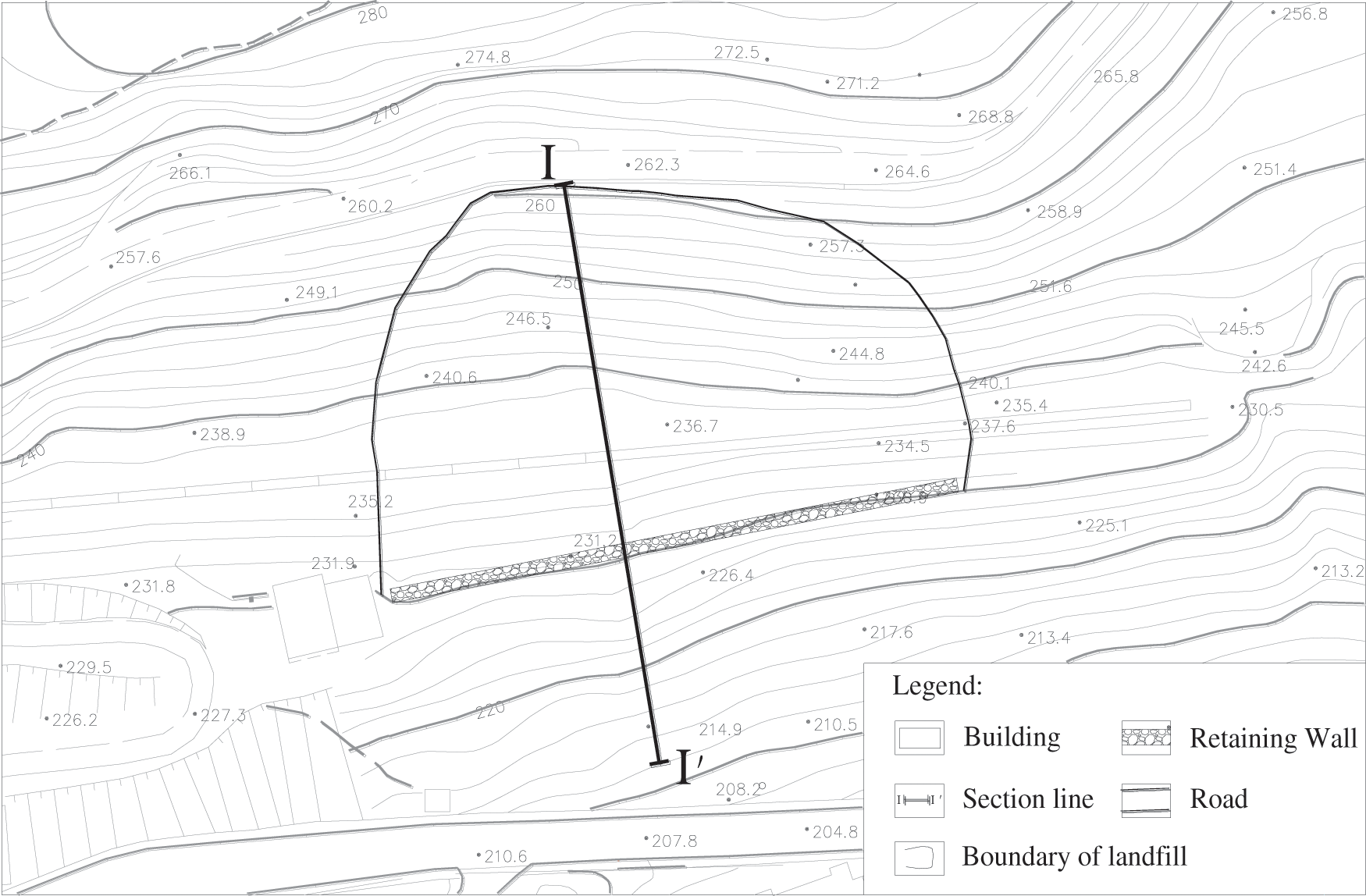
Figure 9: Landfill area layout
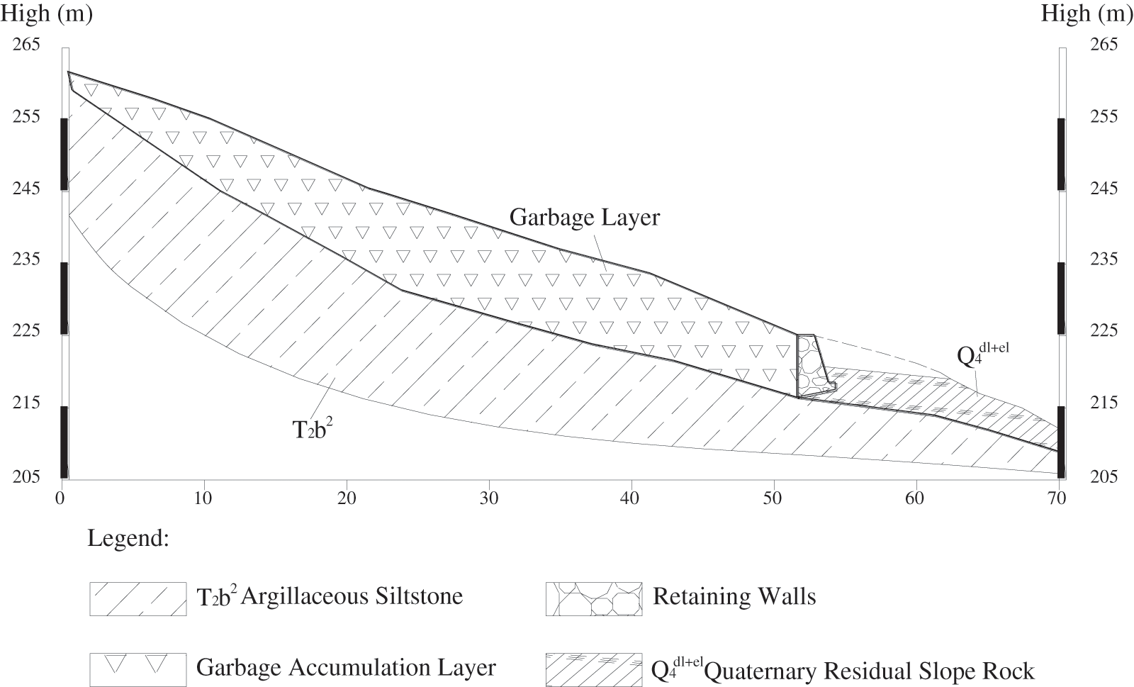
Figure 10: Section I-I of landfill
The analytical model was established according to profile I-I of the Guandukou Town landfill (see Fig. 2). The unit weight of the waste was taken as
The dimensions and angles of the landfill ABCDP are as follows: AB = 54.3 m, AP = 1.3 m, PD = 26.9 m, DC = 28.8 m, BC = 4.3 m,
The dimensions and angles of the retaining wall are as follows: EB = 1.2 m, BC = 4.3 m, CF = 2.4 m, FE = 4.1 m and
6.2.2 Stress and Strain Fields in Landfill
Eighteen coefficients were determined for the landfill solutions under the condition that the force boundary conditions and stress differential equilibrium equations are satisfied. Their values for the stress field (see Fig. 11c) are as follows:
The parameters of the Duncan-Chang constitutive model are as follows:
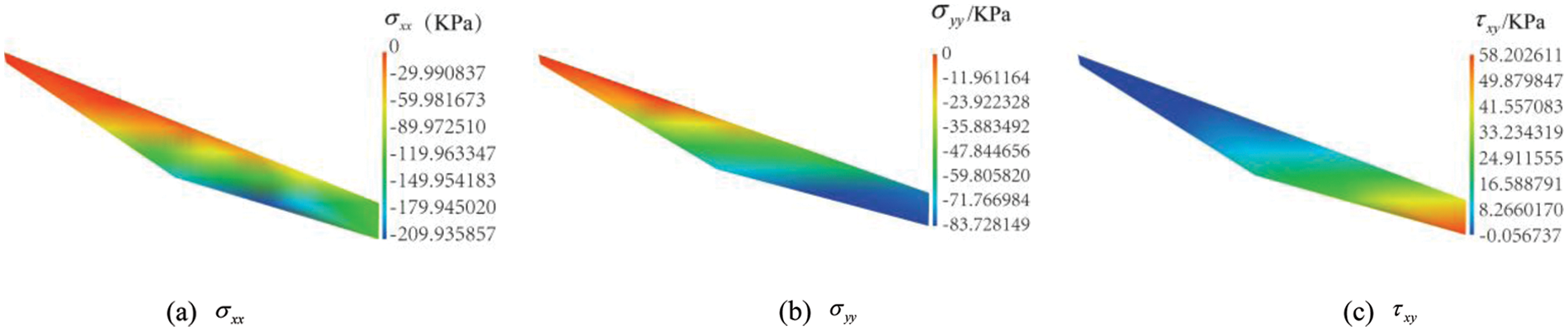
Figure 11: Distributions of stresses
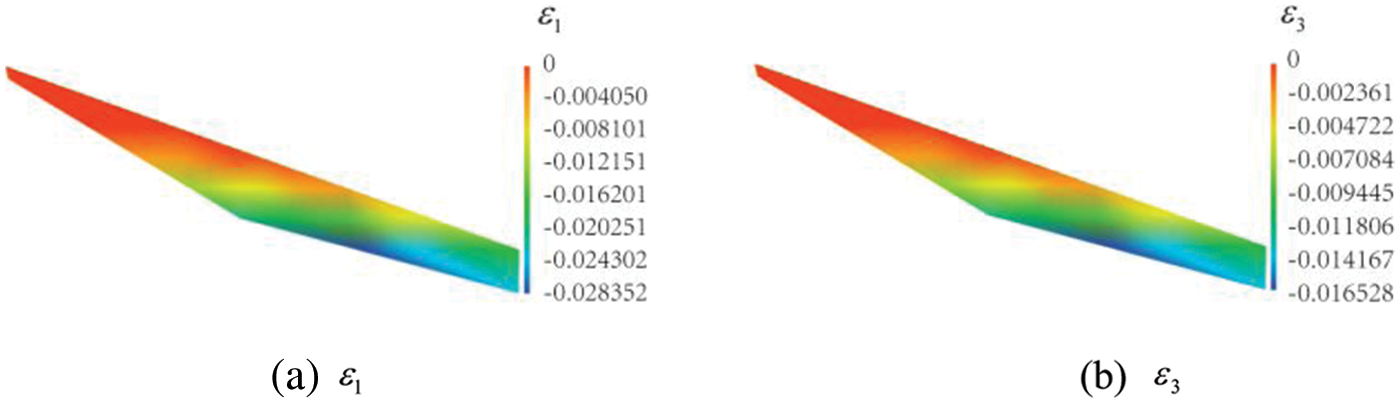
Figure 12: Distributions of principal strains

Figure 13: Distributions of strains
The unit weight of the retaining wall was assumed as
The stress and principle stress fields in the retaining wall are presented in Figs. 14a–14e. If the peak stress in the retaining wall meets the Mohr-Coulomb criterion and the friction angle is taken as
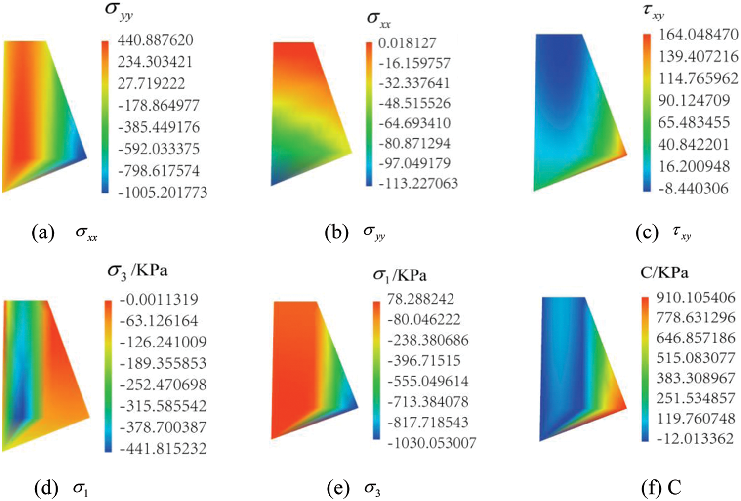
Figure 14: Distributions of stresses
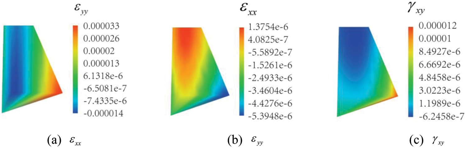
Figure 15: Distributions of strains
6.2.4 Analysis of Results for Landfill with Retaining Wall
6.2.4.1 Landfill Stress and Strain Field Characteristics
The obtained stress and strain fields in the landfill are logical. Stresses
6.2.4.2 Strength Distribution Characteristics in Retaining Wall
The conventional factor of safety against sliding (i.e.,
From the results of the proposed method, it can be seen that the maximum tensile stress is located at point B (78.2 kPa). This value is lower than the strength of M15 mortar and block stone used in the project. The maximum compressive stress (1005 kPa) is located at point F of the retaining wall, which is less than the strength of the retaining wall material. At any point in the retaining wall, the cohesion intercept (C) value is less than 910 kPa (see Fig. 14f) for the internal friction angle of
The ANSYS finite element software was also employed to study the stresses and strains within the landfill and the retaining wall (see Fig. 16). The normal displacement constraints along boundary segments CF, CD, and DP were applied. The differences between the results of the finite element model and the method proposed in this paper were less than 15% for the landfill and 7% for the retaining wall, respectively. The factors of safety for stability along the interface between the retaining wall and its base were also determined and found to differ by more than 5% (see Fig. 17). Note that
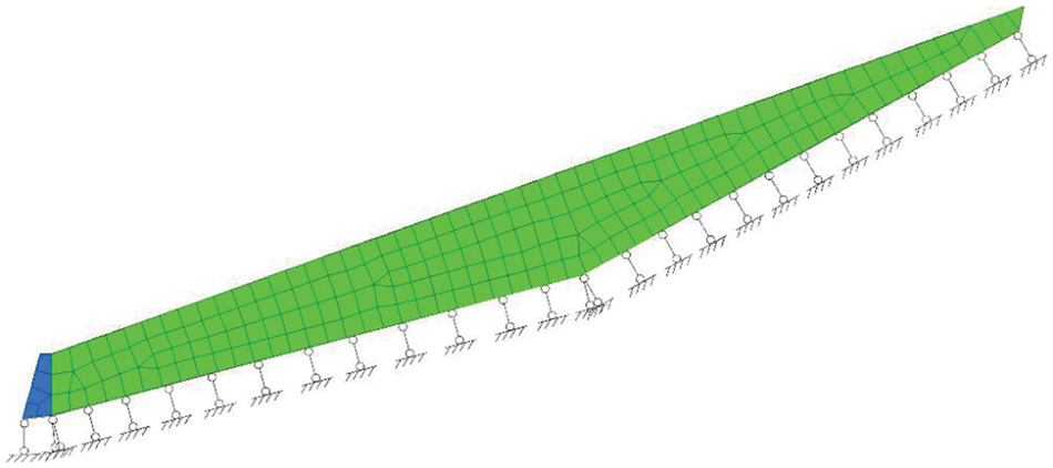
Figure 16: FEM of landfill with retaining wall

Figure 17: Factor of safety at the interface of retaining wall and base
Based on the traditional analysis of the retaining wall (the limited rigid body balance method and FEM) and the proposed methods in this paper, the studied retaining wall is in a stable condition.
(1) The stress and strain field characteristics of the landfill and the retaining wall have been determined. The following conclusions can be drawn: The stress fields in the landfill and the retaining wall are non-linear within the domain. The analytical method proposed in this article can provide a theoretical basis for the control design and displacement prediction of a slope and a retaining wall. Based on the geometry and material of the retaining wall, novel methods for preventing retaining wall failures can be proposed and validated.
(2) The analytical solutions presented in this article are based on the assumption that the stresses are continuous or discontinuous. It is acceptable that the results of the proposed method in this paper are comparable to that of the finite element method under the given boundary conditions.
(3) In this article, the limit equilibrium state hypothesis was ignored for the retaining wall. The stresses acting on the retaining wall included normal stress and the shear stress.
(4) The design methodology of the retaining wall was explained using the results of the numerical analysis. According to the analytical results, the tensile and bulging failure characteristics of the retaining wall and the landfill can be determined. The internal failure of the retaining wall and the landfill can be conducted at any point within the domain, and therefore a new stability analysis method for the anti-sliding design was proposed.
Funding Statement: This work was supported by the National Key R&D Program (No. 2018YFC1504901), and by the Natural Science Foundation of China (Grant No. 42071264). This work was also supported by the Geological Hazard Prevention Project in The Three Gorges Reservoirs (Grant No. 0001212015CC60005).
Conflicts of Interest: The authors declare that they have no conflicts of interest to report regarding the present study.
References
1. Aurelian, T. C., Toshitaka, K., Roy Sidle, C., Mihail, P. (2007). Seismic retrofit of gravity retaining walls for residential fills using ground anchors. Geotechnical and Geological Engineering, 25(6), 679–691. DOI 10.1007/s10706-007-9140-9. [Google Scholar] [CrossRef]
2. Du Bois, A. J. (1879). Upon a new theory of the retaining wall. Pergamon, 108(6), 361–387. DOI 10.1016/0016-0032(79)90345-4. [Google Scholar] [CrossRef]
3. Okabe, S. (1829). General theory of earth pressure. Journal of Japan Society Civil Engineers, 12(1), 311. [Google Scholar]
4. Mononobe, N., Matsuo, H. (1929). On the determination of earth pressure during earthquakes. Proceedings of the World Engineering Conference, pp. 176. Tokyo, Japan. [Google Scholar]
5. Terzaghi, K. (1936). A fundamental fallacy in earth pressure computations. Journal of Boston Society of Civil Engineering, 23, 71–88. [Google Scholar]
6. Kezdi, A. (1958). Earth pressure on retaining wall tilting about the toe. Proceedings of the Brussels Conference on Earth Pressure Problems, pp. 116–132. Brussels, Belgium. [Google Scholar]
7. Handy, R. L. (1985). The arch in soil arching. Journal of Geotechnical Engineering, 111(3), 302–318. DOI 10.1061/(ASCE)0733-9410(1985)111:3(302). [Google Scholar] [CrossRef]
8. Motta, E. (1994). Generalized Coulomb active-earth pressure for distanced surcharge. Journal of Geotechnical Engineering, 120(6), 1072–1079. DOI 10.1061/(ASCE)0733-9410(1994)120:6(1072). [Google Scholar] [CrossRef]
9. Fellenius, W. (1936). Calculation of the stability of the earth dams. Washington. https://www.semanticscholar.org/paper/Calculation-of-stability-of-earth-dam-Fellenius/856680d34954e7bb9dfd1ac7acccf6daee307ecb. [Google Scholar]
10. Bishop, A. W. (1955). The use of the slip circle in the stability analysis of slopes. Géotechnique, 5(1), 7–17. DOI 10.1680/geot.1955.5.1.7. [Google Scholar] [CrossRef]
11. Spencer, E. (1967). A method of analysis of the stability of embankments assuming parallel inter-slice forces. Géotechnique, 17(1), 11–26. DOI 10.1680/geot.1967.17.1.11. [Google Scholar] [CrossRef]
12. Janbu, N. (1973). Slope stability computations. pp. 47–86. NY: John Wiley and Sons Inc. [Google Scholar]
13. Sarma, S. K., Tan, D. (2006). Determination of critical slip surface in slope analysis. Géotechnique, 56(8), 539–550. DOI 10.1680/geot.2006.56.8.539. [Google Scholar] [CrossRef]
14. Kelesoglu, M. K. (2016). The evaluation of three-dimensional effects on slope stability by the strength reduction method. KSCE Journal of Civil Engineering, 20(1), 1–14. DOI 10.1007/s12205-015-0686-4. [Google Scholar] [CrossRef]
15. Gharti, H. N., Komatitsch, D., Oye, V., Martin, R., Tromp, J. (2012). Application of an elastoplastic spectral-element method to 3D slope stability analysis. International Journal for Numerical Methods in Engineering, 91(1), 1–26. DOI 10.1002/nme.3374. [Google Scholar] [CrossRef]
16. Tiwari, R. C., Bhandary, N. P., Yatabe, R. (2015). 3D SEM approach to evaluate the stability of large-scale landslides in Nepal Himalaya. Geotechnical and Geological Engineering, 33(4), 773–793. DOI 10.1007/s10706-015-9858-8. [Google Scholar] [CrossRef]
17. Baker, R. (2004). Nonlinear Mohr envelopes based on triaxial data. Journal of Geotechnical and Geoenvironmental Engineering, 130(5), 498–506. DOI 10.1061/(ASCE)1090-0241(2004)130:5(498). [Google Scholar] [CrossRef]
18. Matthews, C., Farook, Z., Helm, P. (2014). Slope stability analysis-limit equilibrium or the finite element method. Ground Engineering, 48(5), 22–28. [Google Scholar]
19. Faramarzi, L., Zare, M., Azhari, A., Tabaei, M. (2016). Assessment of rock slope stability at Cham-Shir Dam Power Plant pit using the limit equilibrium method and numerical modeling. Bulletin of Engineering Geology and the Environment, 76, 783–794. DOI 10.1007/s10064-016-0870-x. [Google Scholar] [CrossRef]
20. Nilsen, B. (2016). Rock slope stability analysis according to Eurocode 7, discussion of some dilemmas with particular focus on limit equilibrium analysis. Bulletin of Engineering Geology and the Environment, 76(4), 1229–1236. DOI 10.1007/s10064-016-0928-9. [Google Scholar] [CrossRef]
21. Thiebes, B., Bell, R., Glade, T., Stefan, J., Malcolm, A. et al. (2013). A WebGIS decision-support system for slope stability based on limit-equilibrium modelling. Engineering Geology, 158(3), 109–118. DOI 10.1016/j.enggeo.2013.03.004. [Google Scholar] [CrossRef]
22. Antao, A. N., Santana, T. G., da Silva, M. V., da Costa Guerra, N. M. (2011). Passive earth-pressure coefficients by upper-bound numerical limit analysis. Canadian Geotechnical Journal, 48(5), 767–780. DOI 10.1139/t10-103. [Google Scholar] [CrossRef]
23. Benmeddour, D., Mellas, M., Frank, R., Mabrouki, A. (2012). Numerical study of passive and active earth pressures of sands. Computers and Geotechnics, 40(6), 34–44. DOI 10.1016/j.compgeo.2011.10.002. [Google Scholar] [CrossRef]
24. Locat, A., Jostad, H. P., Leroueil, S. (2013). Numerical modeling of progressive failure and its implications for spreads in sensitive clays. Canadian Geotechnical Journal, 50(9), 961–978. DOI 10.1139/cgj-2012-0390. [Google Scholar] [CrossRef]
25. Lu, Y. F., Tu, M. Y., Liu, D. F. (2013). A new joint constitutive model and several new methods of stability coefficient calculation of landslides. Chinese Journal of Rock Mechanics and Engineering, 32(12), 2431–2438. [Google Scholar]
26. Lu, Y. F., Huang, X. B., Liu, D. F. (2017). Distribution characteristics of force and stability analysis of slope. Chinese Journal of Geotechnical Engineering, 39(7), 1321–1329. DOI 10.11779/CJGE201707019. [Google Scholar] [CrossRef]
27. Lu, Y. F. (2015). Deformation and failure mechanism of slope in three dimensions. Journal of Rock Mechanics and Geo-Technical Engineering, 7(2), 109–119. DOI 10.1016/j.jrmge.2015.02.008. [Google Scholar] [CrossRef]
28. Yerro, A., Pinyol, N. M., Alonso, E. E. (2016). Internal progressive failure in deep-seated landslides. Rock Mechanics and Rock Engineering, 49(6), 2317–2332. DOI 10.1007/s00603-015-0888-6. [Google Scholar] [CrossRef]
29. Kwok, O. L. A., Guan, P. C., Cheng, W. P., Sun, C. T. (2015). Semi-Lagrangian reproducing kernel particle method for slope stability analysis and post-failure simulation. KSCE Journal of Civil Engineering, 19(1), 107–115. DOI 10.1007/s12205-013-0550-3. [Google Scholar] [CrossRef]
30. Dawson, E. M., Roth, W. H., Drescher, A. (1999). Slope stability analysis by strength reduction. Geotechnique, 49(6), 835–840. DOI 10.1680/geot.1999.49.6.835. [Google Scholar] [CrossRef]
Appendix
The moment analysis is presented below; for force lever arms see Fig. 7.
Segment BC:
Any point Q is chosen, X’ coordinate is between X’C and X’G, and the lever arm of
Any point S is chosen, X’ coordinate is between X’G and X’B, and the lever arm of
The lever arm of
Segment CF:
(1) Any point V is chosen, X’ coordinate is between X’C and X’P, and the lever arm of
The equation of straight line CF is
(2) Any point X is chosen, X’ coordinate is between X’P and X’F, and the lever arm of
The equation of straight line CF is
The lever arm of
Cite This Article
 Copyright © 2023 The Author(s). Published by Tech Science Press.
This work is licensed under a Creative Commons Attribution 4.0 International License , which permits unrestricted use, distribution, and reproduction in any medium, provided the original work is properly cited.
 Downloads
 Citation Tools