Lightweight Network Ensemble Architecture for Environmental Perception on the Autonomous System

1  Introduction

Ensemble learning is widely considered to be a good way to strengthen generalization ability. It has a wide application in many fields such as visual tracking [1], object detection [2,3], data classification and recognition [4,5], and context processing [6]. Neural network ensemble [7–9] stacks a finite number of neural networks and trains them for the same task, as shown in Fig. 1. Although this parallel ensemble architecture could accurately extract environmental information in complex environment, it is unsuitable for real-time applications on the autonomous system. On the one hand, ensemble architecture does not meet the real-time requirement for real-time applications. For the parallel ensemble architecture, the same input is fed into each component neural network one by one during prediction. This process needs to spend lots of extra time. On the other hand, ensemble architecture dramatically increases the model complexity and requires a lot of memory to run. This poses a great challenge for embedded devices with limited computing resources. Therefore, how to design an effective network ensemble architecture that has less computing time while maintaining the ability of ensemble learning is a challenging problem.

Figure 1: Structure of ensemble learning

To apply the network ensemble architecture to real-time tasks on the autonomous systems, a diffusive network ensemble architecture named PSENet is designed to quickly extract environmental information while maintaining good generalization ability and less parameters. PSENet uses fully shared module, partially shared module, independent module to fuse all component neural networks into one big network. Only one image passes through the above three modules in turn and simultaneously outputs the prediction results of each component network. PSENet could decrease the model complexity and accelerate the computing speed during inference. Moreover, to maintain generalization ability, a training method is designed to train the ensemble architecture and solve the dilemma between single input and multiple outputs in different sub-training sets. Section 3 will introduce PSENet in detail.

The main innovations of this paper are:

1)   A lightweight network ensemble architecture named PSENet is designed and applied to real-time vision tasks on the autonomous system. Compared with parallel ensemble structure, PSENet compresses the model scale and accelerate the inference speed while maintaining generalization ability.

2)   As an extensible network ensemble structure, lots of lightweight neural networks can be put into PSENet to form a lightweight network ensemble structure for real-time applications.

2  Related Works

Ensemble learning combines several weak classifiers as a strong classifier to improve generalization ability. At present, ensemble learning is mainly divided into two categories: (1) traditional machine learning algorithm ensemble such as RF [10] and (2) neural network ensemble. As for parallel machine learning algorithm ensemble, the generation of component learners needed to be designed by ID3 [11], C4.5 [12] and CART. Those traditional methods achieved good performance for simple vision tasks. However, those extracted features were limited by the manual design. So, they couldn't deal with complex tasks such as semantic segmentation in complex conditions. Neural network could learn and adjust weights to adapt to different conditions. So, facing most of complex tasks like object detection and semantic segmentation, neural network ensemble tended to show better performance.

Neural network ensemble comes from [13], which demonstrated that the generalization ability of a neural network system could be significantly improved through ensembling a number of neural networks. Since ensemble structure has good generalization performance, it had been widely adopted in many fields [14–17] and was classified into 3 categories. The first category was the combination of neural networks and traditional ensemble algorithms. Neural networks were used as feature extractors to extract multi-scale features and then those features were fed into the classifiers composed of traditional ensemble algorithms [18–21]. The second category was that neural networks were used as component learners. New neural network was designed to to improve individual performance and then a number of neural networks were stacked as parallel component learners [9,22–24]. This was a common method to improve ensemble performance by improving the performance of individual learners. To expand the differences among component neural networks, incorporating two, two-and-a-half and three-dimensional architecture will strengthen generalization ability [25]. Those methods mentioned in second category produced lots of parameters and slowed down inference speed. BENN [26], a neural network ensemble of Binarized Neural Network [27,28], had few parameters and less inference time meanwhile maintaining a better performance with high accuracy due to a fact that Binarized Neural Network had the potential advantages of high model compression rate and fast calculation speed. However, compared with Binarized Neural Network, BENN produced lots of additional parameters and increase additional inference time. The third category was how to train the component neural networks. The most prevailing approaches were Bagging [29] based on Bootstrap [30] and Boosting [31,32]. In addition, data disturbance such as sample disturbance and parameter disturbance was usually used to increase diversity of component neural networks [33–35]. There is no doubt that most of researches of the neural network ensemble were focused on how to improve the generalization ability and accuracy. For complex tasks in complex conditions, they could achieve good and stable results. However, those methods needed to spend lots of time to predict results. After ensembling m component neural networks, the inference speed would be m times larger than that of a component neural network. Therefore, lightweight neural network ensemble was no longer a lightweight network and was unsuitable for real-time applications on the autonomous system. Although ensemble pruning [36,37] could remove some component neural networks to reduce storage-spend and inference-time-spend, it was extremely limited in many situations and possible to decrease the network ensemble performance. Besides, research on ensemble strategy and generation of component learners, how to design a neural network ensemble architecture with few parameters and less computing time has wide applicability and far-reaching significance.

3  Proposed Algorithm

3.1 Neural Network Ensemble

In this section, we describe the proposed neural network ensemble architecture in detail. In all experiments, we choose bagging to train the component neural networks and choose plurality voting as the combination strategy. To our knowledge, the neural network ensemble usually stacks a number of neural networks that are parallel with each other, as shown in Fig. 2.

Figure 2: Neural network ensemble architecture

Lots of parallel neural networks make the neural network ensemble architecture become very wide, which leads to two problems. The first problem is lots of parameters. When the neural network ensemble consists of n component neural networks, its parameters will be n times larger than that of a component neural network. This poses a challenge to the storage of embedded AI computing devices. The second problem is inference time. Component neural networks are independent of each other and are run one by one. Those need to spend lots of meaningless time. If there are n component neural networks, when we use the neural network ensemble to predict results, all component neural networks need to be calculated in turn and its inference time is n times larger than that of a component neural network. Slow inference speed limits the applications of neural network ensemble architecture in real-time tasks.

Three conditions are considered: (1) the ability of ensemble learning requires network ensemble architecture to consist of a number of parallel component neural networks, (2) less computing time requires all component neural networks to reason the results simultaneously, and (3) few parameters require component neural networks to share finite layers. Strong generalization ability is the main advantage of the ensemble architecture. Here, the main research focuses on how to accelerate the inference speed while maintaining generalization ability. Starting from the generalization ability, the disagreement between different component networks is explored. When two component networks share partial layers to extract initial features, they also maintain large disagreement. Based on this discovery, a diffusive network ensemble architecture named PSENet is proposed. PSENet consists of fully shared module, partially shared module, and independent module. Shared module is to decrease the parameters and connect input to each component neural network, including fully shared module and partially shared module. Fully shared module is a common module shared by all component neural networks, being directly connected to the input. As a connecting hub, it provides all component neural networks with the same input. Partially shared module, a module shared by partially component neural networks, is to decrease the parameters and mitigate the relevance among component neural networks. Independent module, usually placed at the end of the encoder, has lots of parallel branches and plays an important role in maintaining the independence among component neural networks. When the vision task is the semantic segmentation task, the next module following independent layer is the upsampling [38–40]. When the vision task is the classification task, the next module following independent layer is the classifier. Firstly, the input image is fed into the fully shared module to extract initial features. Fully shared module, including several consecutive layers named as fully shared layers, only consists of one branch. Several component networks share a same initial feature extraction module to decrease the model complexity, computing time, and parameters. Then, the initial features are fed into the partially shared module. Partially shared module consists of several parallel branches which are connected to the branch from fully connected module. Finally, features extracted by partially shared module are fed into the independent module. Independent module consists of lots of branches which have as many as component neural networks, and usually is placed at the end of the encoder. Its main role is to extract different features for each component network and ensure that each component network is independent of each other to maintain the generalization ability. From input to output, above three modules are connected in turn, which fuse all parallel component neural networks into one network, as shown in Figs. 3–5. The neural network ensemble architecture, called full-full-full architecture, as shown in Fig. 3, consists of three fully shared modules, followed one classier layer. Above three fully shared modules extract spatial features that are fed into component neural networks. Compared with traditional neural network ensemble architecture, this architecture has fewer parameters and quicker inference speed, but it significantly weakens the generalization ability. The neural network ensemble architecture, called full-full-partial architecture, as shown in Fig. 4, consists of two fully shared modules, one partially shared module. Compared with full-full-full architecture, full-full-partial architecture adds the partially shared module which enhances the diversity of the extracted features to a certain extent. Therefore, full-full-partial architecture strengthens the independence among component neural networks by adding intermediate module (partially shared module) and has stronger generalization ability than full-full-full architecture. The neural network ensemble architecture, called full-partial-independent architecture, as shown in Fig. 5, consists of one fully shared module, one partially shared module, and one independent module. Each branch of independent module is parallel with each other and is trained independently. This is beneficial to strengthen the diversity of component neural networks and maintain the independence among component neural networks. However, lots of parallel branches produce more parameters. Moreover, full-partial-independent architecture, mixing multiple modules that are distributed in different stages, is difficult to be trained.

Figure 3: Proposed neural network ensemble architecture with three fully shared modules. This architecture is called as full-full-full

Figure 4: Proposed neural network ensemble architecture with two fully shared modules and one partially shared module. This architecture is called as full-full-partial

Figure 5: Proposed neural network ensemble architecture with one fully shared module, several partially shared modules and several independent modules. This architecture is called as full-partial-independent

3.2 Training Method

In order to maintain the disagreement among component networks, all component networks need to be trained in different sub-training datasets to obtain different feature representations. PSENet has only one input connected with multiple component networks. If it is seen as a whole to train, component networks will learn similar features and lose ensemble ability. The learning of neural networks includes forward propagation and back propagation [41]. Generally, a combination of forward propagation and back propagation completes one update of parameters. Different from the traditional neural network ensemble architecture, the proposed neural network ensemble architecture fuses a number of component neural networks into one network and all/some component neural networks have some shared layers. This causes that those shared parameters cannot be updated only by a component training dataset. Besides, to strengthen generalization ability, component neural networks are trained in different training subsets. So multiple forward propagation followed by one back propagation completes an update of the neural network ensemble. Here, each forward propagation only propagates in the corresponding component neural network and the direction of each forward propagation is controlled by the connection among fully shared layers, partially shared layers, and independent layers. Through forward propagation, we can get the predicted results of the component learner:

Hj=FD(Dj),Dj⊆D(1)

where Hj is the prediction result on jth training subset. F is the function of component neural network. Dj is the training subset produced by bootstrap sampling. D is training set. The loss of each component neural network can be expressed by:

Lj=Floss(Hj,Tj)(2)

Floss is the loss function. Tj is the corresponding labels. Due to all component neural networks have the same structure and task, we take the average of losses from corresponding component neural networks as the final loss for back propagation.

L=1n∑j=1nLj(3)

The proposed neural network ensemble architecture mixes the fully shared layers, partially shared layers, and independent layers and it is inappropriate to regard the encoder as a whole to train. Here, we divide encoder into several stage and fully shared layers, partially shared layers, and independent layers are trained one by one. Eq. (1) is expressed by the following formula:

Hj=Fωi(Fωp(Fωf(Dj))),Dj⊆D(4)

where Fωf, Fωp, and Fωi are the non-linear relationships about fully shared layers, partially shared layers, and independent layers, respectively. Here, three stages are used to train the weights. The first stage is to train the fully shared layers and all training data are fed into a component neural network. After the training of fully shared layers, the weights of fully shared layers in the component learner are directly transplanted to the fully shared layers in the network ensemble architecture.

The second step is to train the partially shared modules. In this step, the weights of fully shared layers are fixed and other weights are initialized randomly. Several training subsets are obtained by the Bootstrap method. Eq. (4) is expressed by the following formula:

Hj=Fωi(FI,ωp(Ff(Dj))),Dj⊆DI(5)

where Ff() is the fully shared layers with fixed weights in the component learners. DI is the Ith training subset. FI,ωp is the partially shared layers in the Ith partially shared module that need to be trained in the Ith training subset. The training process of partially shared modules is shown in Algorithm 1.

The third step is to train the independent modules. In this step, the weights of fully shared layers and partially shared layers are fixed and other weights are initialized randomly. According to the Bootstrap method, the training dataset is divided into subsets as many as the component neural networks. Eq. (4) is expressed by the following formula:

Hj=FJ,I,ωi(FI,p(Ff(Dj))),Dj⊆DJ(6)

where FI,p is the Ith partially shared module with fixed weights. FJ,I,ωi is the independent layers in the Jth independent module that is directly connected to the Ith partially shared module, which need to be trained in the Jth training subset. The training process of independent modules is shown in Algorithm 2.

3.3 Diversity Measure of Component Neural Networks

Disagreement measure is used to evaluate the diversity measure of component neural networks. For a given dataset D={(x1,y1),(x2,y2),⋅⋅,(xn,yn)}, facing the multiple categories task, there exists yi∈{0,1,⋅⋅,m−1,m} and we can get the contingency table between any two component neural networks named as M and N respectively, as shown in Table 1.

Here, bi,j is the number of the samples when M = i and N = j. The disagreement measure between any two component neural networks can be expressed by:

disi,j=∑i=jbi,j∑i=0m∑j=0mbi,j(7)

In terms of neural network ensemble architecture, it consists of lots of component neural networks. Therefore, we get the statistics as the disagreement measure of neural network ensemble:

dis=∑i=0m−1∑j=i+1mdisi,j∑k=1mk(8)

4  Experimental Results

We evaluate the performance of the PSENet on Camvid [42,43] and CIFAR-10 [44] with the traditional parallel neural network ensemble architecture in terms of accuracy, parameters, inference speed, and disagreements measure. In this section, through several experiments, we prove the relationships and roles between different stages. Besides, compared with parallel neural network ensemble, we show the advantages of the proposed neural network ensemble architecture.

4.1 Performance Evaluation on the Camvid Dataset

The Camvid dataset consists of 701 color-scale road images collected in different locations. For easy and fair comparison with prior work, we adopt the common split [45]. Training dataset includes 367 images, validation dataset includes 101 images and testing dataset includes 233 images. Segmenting 11 classes on the Camvid Dataset is used to verify performance.

We divide the training dataset into a lot of component training datasets which include 220 images randomly selected from 367 images and are used to train independent layers. Besides, we make some special component training datasets, including 220 images randomly selected from the several corresponding component training datasets, to train the shared modules. Here, a random self-designed neural network is used as the component neural network to do ablation experiment, as shown in Fig. 6.

Figure 6: Random self-designed neural network

On the basis of this component neural network, we stack many component neural networks to build a traditional neural network ensemble architecture and build several proposed neural network ensemble architecture. To show the performance between different neural network ensemble architecture, we design an ablation experiment and the results are shown in Table 2. In Table 2, we design 7 experiments on different neural network structures. One of them is used as a parallel neural network ensemble and the rest remaining structures belong to different proposed neural network ensemble architectures. We measure the performance of different networks by Mean Intersection over Union (MIoU), disagreement measure, FPS, and parameters. The “full”, “partial”, and “-” expresses the fully shared modules, the partially shared module, and the independent module respectively. The “partial3” expresses that partially shared module includes 3 shared branches. The “independent3-9” expresses that the first half of the independent module includes 3 shared branches, and the second half includes 9 independent branches.

The parallel neural network ensemble significantly improves the generalization ability of neural networks and produces higher accuracy that is higher 3.1 MIoU than that of component neural networks, but it produces lots of parameters due to the factor that it stacks lots of component neural networks. Besides, component neural networks are independent of each other and are run one by one. So, we need to repeatedly feed the same input into the different component neural networks when we reason the results. Fully shared module is directly connected to the input and shared by all component neural networks, so we can simultaneously run all component neural networks with only one input. This will accelerate inference speed and save much inference time. From Table 2, compared with traditional neural network ensemble, the neural network ensemble with fully shared module could spend less time to complete the same task. The encoder of the proposed neural network ensemble architecture includes three modules: fully shared module, partially shared module, and independent module. Fully shared module could decrease the parameters and accelerate inference speed, but it makes all component neural networks become similar to each other. So too many fully shared modules (fully shared layers) make neural network ensemble lose the ability of the ensemble (generalization ability). Independent module tends to make all component neural networks become independent of each other, but it produces lots of parameters and slows down the inference speed. The performance of partially shared module is between fully shared module and independent module. It tends to make a trade-off between inference speed and accuracy. Full-independent-independent has similar accuracy, disagreement measure, and parameters to traditional neural network ensemble. However, in terms of inference speed, it is 1.89 times quicker than that of traditional neural network ensemble. This demonstrates that the combination of too many independent layers and fully shared layers will accelerate the inference speed meanwhile maintaining the excellent performance of traditional neural network ensemble. When we replace the independent module with the partially shared module, the inference speed is further accelerated due to the reduction of some branches. However, the accuracy will decrease accordingly. With the increase of fully shared module, although the inference speed and parameters of the neural network ensemble are improved, the accuracy and disagreement measure will decrease a lot. When three stages consist of fully shared module, the neural network ensemble basically loses integration ability.

Table 3 shows the disagreement measure between any two component neural networks in full-full-partial. Here, partially shared module consists of three branches and each branch is directly connected to three classifiers. When one branch is shared by several classifiers in stage 3, the corresponding component neural networks are similar. From Table 3, every three component neural networks have similar performance and basically lose integration ability. This results in that some component neural networks are redundant and has little effect on the ensemble ability.

Other neural networks like FCN [46], ENet [47], and DABNet [48], BiseNet [49] are used as component neural networks respectively and we stack them to build different traditional neural network ensemble architecture. And then we compare the corresponding proposed neural network ensemble architecture with parallel neural network ensemble architecture in terms of ensemble accuracy, inference speed, and parameters. The results are shown in Table 4. With the increase of the shared layers, the neural network ensemble architecture produces few parameters and accelerates the inference speed (FPS). However, its diversity is also decreased. So, a finite number of shared layers followed by enough independent layers produce quick inference speed and few parameters while maintaining ensemble accuracy.

Ensemble accuracy. Ensemble architecture has better generalization ability and tends to produce high accuracy. In parallel neural network ensemble architecture, component neural networks are parallel, which makes the component neural networks independent of each other. The parallel architecture is benefit to strengthen the ensemble ability. Based on the parallel network ensemble architecture, the proposed network ensemble architecture fuses parallel component neural networks into a big ensemble architecture in which all component neural networks could predict the results with only one input. From Table 4, compared with parallel architecture, full-partial-independent architecture achieves similar accuracy while having simple model complexity.

Inference speed. Component neural networks in the parallel ensemble architecture predict the results one by one. Besides, each forecast result of the component neural network needs to input the same data repeatedly. This results in the cost of much extra time. Full-partial-independent architecture changes the reasoning method. All component neural networks are connected to the fully shared module. So when one input is fed into the full-partial-independent architecture, all component neural networks could predict the results simultaneously. From Table 4, full-partial-independent architecture has the obvious advantage than parallel architecture in terms of inference speed. For example, when FCN is used as component neural network, the inference speed of full-part-independent is 3.2 times quicker than that of parallel neural network ensemble architecture while maintaining high ensemble accuracy as parallel network ensemble architecture. When ENet is used as component neural network, the advantage of full-part-independent architecture is weakened in terms of inference speed that is 1.5 times quicker than that of traditional neural network ensemble architecture due to lots of independent layers.

Parameters. Component neural networks in parallel ensemble architecture are independent with each other. In full-partial-independent architecture, all/some component neural networks have some shared layers. So compared with parallel ensemble architecture, full-partial-independent architecture has fewer parameters.

4.2 Performance Evaluation on the CIFAR-10 Dataset

The CIFAR-10 Dataset consists of 60000 32 × 32 color images. Training dataset includes 50000 images and testing dataset includes 10000 images. This dataset has 10 classes containing 6000 images each. There are 5000 training images and 1000 testing images per class.

Similarly, we divide the training dataset into a lot of component training datasets which include 30000 images randomly selected from 50000 images and are used to train independent layers. Neural networks like MobileNet [50], Xception [51], and SqueezeNet [52] are used as component neural network respectively. On the basis of those component neural networks, we compare parallel neural network ensemble architecture with the proposed neural network ensemble architecture in terms of ensemble accuracy, inference speed, disagreement measure, and parameters. The results are shown in Table 5.

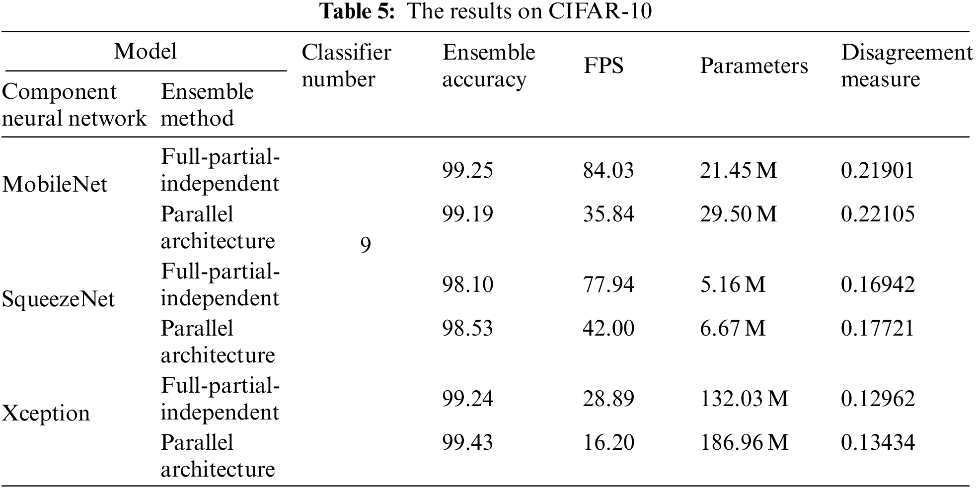
Ensemble accuracy, Inference speed, and parameters. From Table 5, parallel neural network ensemble could improve the accuracy, but it significantly sacrifices the inference speed and produces lots of parameters. When we introduce fully shared module and fuse those parallel component neural networks into one network named full-independent-independent, all component neural networks can be simultaneously run with only one input. This saves much time and accelerates the inference speed. On the basis of full-independent-independent architecture, when we replace an independent module with a partially shared module, inference speed is further accelerated. At the same time, introducing a partially shared module slightly decreases the disagreement measure and full-partial-independent architecture keeps the ensemble accuracy basically consistent with the full-independent-independent architecture. Generally, neural network ensemble architecture could significantly improve the accuracy, but introduces a lot of parameters and slows down the inference speed. The proposed neural network ensemble architecture compresses ensemble architecture and accelerates the inference speed meanwhile keeping the ensemble accuracy basically consistent with the traditional neural network ensemble architecture.

Disagreement measure. Disagreement measures the difference between any two component neural networks. Small disagreement means that any two component neural networks extract similar features, which are adverse to the generalization ability. Parallel architecture has good disagreement, but it leads to many problems such as slow inference speed and lots of parameters. Here, the proposed full-partial-independent architecture mitigate the above problems. Shared modules reduce the parameters and accelerate the inference speed. Independent modules keep component neural networks independent with each other. From Table 5, compared with parallel ensemble architecture, full-partial-independent architecture produces similar disagreement. This reveals that the proposed ensemble architecture has a good generalization ability while producing quick inference speed and few parameters.

4.3 Performance in the Real World

4.3.1 Environment Understanding of Unmanned Robot

In the real world, unmanned robot needs to perform various tasks in different environments. Here, two vision tasks are tested on the unmanned robot to show the PSENet performance. One is the semantic segmentation, a key technology for unmanned robot to understand environmental information. 11 classes such as road, sky, car, building, tree, and so on are segmented from the image. The other is a classification task. According to different targets in the image, the scene is divided into 4 classes: experimental area, garden, parking lot, and main road. The environmental perception system is shown in Fig. 7 and the unmanned robot is shown in Fig. 8.

Figure 7: Environmental perception system

Figure 8: Unmanned system

While the unmanned system is moving, the camera captures the images, and those captured images are transmitted to the AI embedded device. Then PSENet deals with those images in real time and the results are fed back to the unmanned system. Fig. 9 shows some results of semantic segmentation and scene recognition in continuous road scenes.

Figure 9: Results in the real world

Semantic segmentation. In the whole road scenes, a single neural network could better segment large classes such as road, sky, tree, building, and car from the image. However, a lot of noise are existed in each large classes. PSENet synthesizes the results of multiple networks and effectively mitigate the problem. For small classes such as bicyclist, fence, column, both the single neural network and PSENet produce coarse semantic segmentation results. Overall, compared with the single neural network, PSENet achieves smooth boundary and high accuracy.

Classification. The whole road scenes are divided in 4 categories: experimental area, garden, parking lot, main road. The unmanned mobile recognizes different scenes to finish different operations. For example, when passing through the parking lot, the unmanned system can perform parking operation. When passing through the main road, the unmanned system needs to drive to the right and increases its speed appropriately. In road scenes, PSENet could recognize the category of each scene well.

4.3.2 Classification of Tobacco Leaf State during Curing

Intelligent baking requires to identify the drying degree of tobacco leaves and adjust the temperature. Therefore, it is a key technology to accurately identify the current stage of tobacco leaf. The intelligent baking system is shown in the Fig. 10. The CCD camera is used to collect tobacco leaves, and the pictures are transmitted to the processor for processing. Finally, the results are fed back to the controller to adjust the temperature. State discrimination results of tobacco leaves are shown in the Table 6 and Fig. 11.

Figure 10: Intelligent baking system

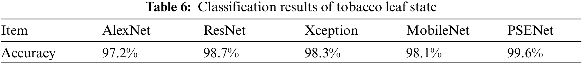
Figure 11: State discrimination results of tobacco leaves

It is necessary for tobacco leaves to adjust the temperature under different baking conditions. Tobacco leaves are divided into 10 states, and each state corresponds to a different baking temperature. The intelligent baking control of tobacco leaf is realized by judging the current tobacco leaf state and adaptively adjusting the baking temperature. For 2217 continuous images, PSENet is used for state recognition. Results in the real world show that PSENet can well distinguish each state of tobacco. As the early method, AlexNet has 95.2% accuracy. ResNet introduces the residual structure and greatly deepens the network structure, so as to obtain better performance. Compared with AlexNet, ResNet could improve the accuracy from 97.2% to 98.7%. Based on Inception V3, Xception simplifies the calculation of convolution. It replaces the standard convolution with the combination of 1 × 1 convolution and separable convolution. For classification of tobacco leaf state, Xception produces 98.3%. MobileNet, a lightweight neural network, produces similar accuracy like Xception. Xception and MobileNet produce lower accuracy than ResNet. However, they achieve a quicker inference speed. As a ensemble architecture, PSENet achieves 99.6% accuracy that outperform other algorithms. For classification of tobacco leaf state, it is difficult to classify the last four stages due to similar appearance. PSENet could overcome this problem and achieve stable and accurate classification results.

5  Conclusions

We present a new lightweight neural network ensemble architecture that compresses the parallel neural network ensemble architecture. This ensemble architecture divides the parallel structure into fully shared module, partially shared module, and independent module. A fully shared module is shared by all component neural networks and makes all component neural networks simultaneously run with only one input. Independent module tends to keep component neural networks independent of each other and makes the neural network ensemble architecture have a good ensemble ability. We test on Camvid and CIFAR-10 and the results show that the proposed neural network ensemble architecture not only decreases the parameters but also significantly accelerates the inference speed while keeping the ensemble ability similar to the parallel neural network ensemble architecture. This revealed that partially shared layers also maintain the independence of the component neural network and have a greater advantage than the parallel ensemble structure. In the real world, PSENet could deal with semantic segmentation and scene recognition well. In the future, the work mainly focuses on how to determine the relationship between various modules such as the number of shared components.

Funding Statement: This work is supported by the National Key Research and Development Program of China under Grant 2019YFC1511401, the National Natural Science Foundation of China under Grant 62173038 and 61103157, Science Foundation for Young Scholars of Tobacco Research Institute of Chinese Academy of Agricultural Sciences under Grant 2021B05, and Key Scientific and Technological Research and Development Project of China National Tobacco Corporation under Grant 110202102007.

Conflicts of Interest: The authors declare that they have no conflicts of interest to report regarding the present study.

References

 1.  Jiang, C. R., Xiao, J. M., Xie, Y. C., Tillo, T., Huang, K. Z. (2018). Siamese network ensemble for visual tracking. Neurocomputing, 275, 2892–2903. DOI 10.1016/j.neucom.2017.10.043. [Google Scholar] [CrossRef]

 2.  Wang, Y. Y., Wang, D. J., Geng, N., Wang, Y. Z., Yin, Y. Q. et al. (2019). Stacking-based ensemble learning of decision trees for interpretable prostate cancer detection. Applied Soft Computing, 77, 188–204. DOI 10.1016/j.asoc.2019.01.015. [Google Scholar] [CrossRef]

 3.  Ghanbari-Adivi, F., Mosleh, M. (2019). Text emotion detection in social networks using a novel ensemble classifier based on parzen tree estimator. Neural Computing and Applications, 31(12), 8971–8983. DOI 10.1007/s00521-019-04230-9. [Google Scholar] [CrossRef]

 4.  Yu, Z. W., Wang, D. X., Zhao, Z. X., Chen, C. L. P., You, J. et al. (2019). Hybrid incremental ensemble learning for noisy real-world data classification. IEEE Transactions on Cybernetics, 49(2), 403–416. DOI 10.1109/TCYB.2017.2774266. [Google Scholar] [CrossRef]

 5.  Ma, X. Q., Liu, W. F., Tao, D. P., Zhou, Y. C. (2019). Ensemble p-laplacian regularization for scene image recognition. Cognitive Computing, 11(6), 841–854. DOI 10.1007/s12559-019-09637-z. [Google Scholar] [CrossRef]

 6.  Krawczyk, B., Mclnnes, B. T. (2018). Local ensemble learning from imbalanced and noisy data for word sense disambiguation. Pattern Recognition, 78, 103–119. DOI 10.1016/j.patcog.2017.10.028. [Google Scholar] [CrossRef]

 7.  Rayal, R., Khanna, D., Sandhu, J. K., Hooda, N., Rana, P. S. (2019). N-Semble: Neural network based ensemble approach. International Journal of Machine Learning and Cybernetics, 10(2), 337–345. DOI 10.1007/s13042-017-0718-0. [Google Scholar] [CrossRef]

 8.  Ke, R. M., Tang, Z. B., Tang, J. J., Pan, Z. W., Wang, Y. H. (2019). Real-time traffic flow parameter estimation from uav video based on ensemble classifier and optical flow. IEEE Transactions on Intelligent Transaction Systems, 20(1), 54–64. DOI 10.1109/TITS.2018.2797697. [Google Scholar] [CrossRef]

 9.  Debapriya, M., Anirban, S., Pabitra, M., Debdoot, S. (2016). Ensemble of deep convolutional neural networks for learning to detect retinal vessels in fundus images. https://arxiv.org/abs/1603.04833v1. [Google Scholar]

10. Breiman, L. (2001). Random forests. Machine Learning, 45(1), 5–32. DOI 10.1023/A:1010933404324. [Google Scholar] [CrossRef]

11. Quinlan, J. R. (1986). Induction of decision trees. Machine Learning, 1(1), 81–106. DOI 10.1007/BF00116251. [Google Scholar] [CrossRef]

12. Quinlan, J. R. (1986). Improved use of continuous attributes in C4.5. Journal of Artificial Intelligence Research, 4, 77–90. DOI 10.1613/jair.279. [Google Scholar] [CrossRef]

13. Hansen, L. K., Salamon, P. (1990). Neural network ensembles. IEEE Transactions on Pattern Analysis and Machine Intelligence, 12(10), 993–1001. DOI 10.1109/34.58871. [Google Scholar] [CrossRef]

14. Chen, F. J., Wang, Z. L., Xu, Z. G., Jiang, X. (2009). Facial expression recognition based on wavelet energy distribution feature and neural network ensemble. 2009 WRI Global Congress on Intelligent Systems, pp. 122–126. Xiamen, China. [Google Scholar]

15. Khened, M., Kolletathu, V. A., Krishnamurthi, G. (2019). Fully convolutional multi-scale residual densenets for cardiac segmentation and automated cardiac diagnosis using ensemble of classidiers. Medical Image Analysis, 51, 21–45. DOI 10.1016/j.media.2018.10.004. [Google Scholar] [CrossRef]

16. Rasp, S., Lerch, S. (2018). Neural networks for postprocessing ensemble weather forecasts. Monthly Weather Review, 146(11), 3885–3900. DOI 10.1175/MWR-D-18-0187.1. [Google Scholar] [CrossRef]

17. Alvarez-Arenal, A., Dellanos-Lanchares, H., Martin-Fernandez, E., Mauvezin, M., Sanchez, M. L. et al. (2020). An artificial neural network model for the prediction of bruxism by means of occlusal variables. Neural Computing and Application, 32(5), 1259–1267. DOI 10.1007/s00521-018-3715-7. [Google Scholar] [CrossRef]

18. Li, T., Leng, J. B., Kong, L. Y., Guo, S., Bai, G. et al. (2019). Dcnr: Deep cube cnn with random forest for hyperspectral image classifification. Multimedia Tools and Applications, 78(3), 3411–3433. DOI 10.1007/s11042-018-5986-5. [Google Scholar] [CrossRef]

19. Ye, J. H., Shi, S. X., Li, H. X., Zuo, J. L., Wang, S. M. (2018). A horizon detection method based on deep learning and random forest. Journal of System Simulation, 30(7), 2507–2514. DOI 10.16182/j.issn1004731x.joss.201807010. [Google Scholar] [CrossRef]

20. Guo, Y. Y., Wang, X., Xiao, P. C., Xu, X. Z. (2020). An ensemble learning framework for convolutional neural network based on multiple classifiers. Soft Computing, 24(5), 3727–3735. DOI 10.1007/s00500-019-04141-w. [Google Scholar] [CrossRef]

21. Li, H. W., Jiang, G. F., Zhang, J. G., Wang, R. X., Wang, Z. L. et al. (2018). Fully convolutional network ensembles for white matter hyperintensities segmentation in MR images. Neuroimage, 183, 650–665. DOI 10.1016/j.neuroimage.2018.07.005. [Google Scholar] [CrossRef]

22. Fu, Q., Dong, H. B. (2021). An ensemble unsupervised spiking neural network for objective recognition. Neurocomputing, 419(2), 47–58. DOI 10.1016/j.neucom.2020.07.109. [Google Scholar] [CrossRef]

23. Fu, G. Y. (2018). Deep belief network based ensemble approach for cooling load forecasting of air-conditioning system. Energy, 148, 269–282. DOI 10.1016/j.energy.2018.01.180. [Google Scholar] [CrossRef]

24. Yu, Z. W., Zhang, Y. D., Chen, C. L. P., You, J., Wong, H. S. (2019). Multiobjective semisupervised classifier ensemble. IEEE Transactions on Cybernetics, 49(6), 2280–2293. DOI 10.1109/TCYB.2018.2824299. [Google Scholar] [CrossRef]

25. Bermejo-Pelaez, D., Ash, S. Y., Washko, G. R., Esteparz, R. S. J., LedesmaCarbayo, M. J. (2020). Classification of interstitial lung abnormality patterns with an ensemble of deep convolutional neural networks. Science Reports, 10(1), 338. DOI 10.1038/s41598-019-56989-5. [Google Scholar] [CrossRef]

26. Zhu, S. L., Dong, X., Su, H. (2019). Binary ensemble neural network: More bits per network or more network per bits?. 2019 IEEE/CVF Conference on Computer Vision and Pattern Recognition (CVPR), pp. 4918–4927. Long Beach, USA. [Google Scholar]

27. Courbariaux, M., Hubara, I., Soudry, D., El-Yaniv, R., Bengio, Y. (2016). Binarized neural networks: Training deep neural networks with weights and activations constrained to +1 or −1. https://arxiv.org/abs/1602.02830. [Google Scholar]

28. Rastegari, M., Ordonez, V., Redmon, J., Farhadi, A. (2016). XNOR-Net: ImageNet classifification using binary convolutional neural networks. 14th European Conference on Computer Vision (ECCV), pp. 525–542. Amsterdam, The Netherlands. [Google Scholar]

29. Breiman, L. (1996). Bagging predictors. Machine Learning, 24(2), 123–140. DOI 10.1007/BF00058655. [Google Scholar] [CrossRef]

30. Markus, M. T., Groenen, P. J. F. (1998). An introduction to the bootstrap. Psychometrika, 63(1), 97–101. DOI 10.1111/1467-9639.00050. [Google Scholar] [CrossRef]

31. Schapire, R. E. (1990). The strength of weak learnability. Machine Learning, 5(2), 197–227. DOI 10.1007/BF00116037. [Google Scholar] [CrossRef]

32. Freund, Y. (1995). Boosting a weak learning algorithm by majority. Information and Computation, 121(2), 256–285. DOI 10.1006/inco.1995.1136. [Google Scholar] [CrossRef]

33. Ho, T. K. (1998). The random subspace method for constructing decision forests. IEEE Transactions on Pattern Analysis and Machine Intelligence, 20(8), 832–844. DOI 10.1109/34.709601. [Google Scholar] [CrossRef]

34. Breiman, L. (2000). Randomizing outputs to increase prediction accuracy. Machine Learning, 45(3), 261–277. DOI 10.1023/A:1017934522171. [Google Scholar] [CrossRef]

35. Liu, Y., Yao, X. (1999). Ensemble learning via negative correlation. Neural Networks, 12(10), 1399–1404. DOI 10.1016/S0893-6080(99)00073-8. [Google Scholar] [CrossRef]

36. Rokach, L. (2010). Ensemble-based classififiers. Artifificial Intelligence Review, 33(1), 1–39. DOI 10.1007/s10462-009-9124-7. [Google Scholar] [CrossRef]

37. Zhou, Z. H., Wu, J. X., Tang, W. (2002). Ensembling neural networks: Many could be better than all. Artificial Intelligent, 137(1), 239–263. DOI 10.1016/S0004-3702(02)00190-X. [Google Scholar] [CrossRef]

38. Keys, R. G. (1981). Cubic convolution interpolation for digital image-processing. IEEE Transactions on Acoustics Speech and Signal Processing, 29(6), 1153–1160. DOI 10.1109/TASSP.1981.1163711. [Google Scholar] [CrossRef]

39. Zeiler, M. D., Krishnan, D., Taylor, G. W., Fergus, R. (2010). Deconvolutional networks. 2010 IEEE Conference on Computer Vision and Pattern Recognition (CVPR), pp. 2528–2535. San Francisco, USA. [Google Scholar]

40. Zeiler, M. D., Taylor, G. W., Fergus, R. (2011). Adaptive deconvolutional networks for Mid and high level feature learning. 2011 IEEE International Conference on Computer Vision (ICCV), pp. 2018–2025. Barcelona, Spain. [Google Scholar]

41. Rumelhart, D. E., Hinton, G. E., Williams, R. J. (1986). Learning representations by back-propagating errors. Nature, 323(6088), 533–536. DOI 10.1038/323533a0. [Google Scholar] [CrossRef]

42. Brostow, G. J., Shotton, J., Fauqueur, J., Cipolla, R. (2008). Segmentation and recognition using structure from motion point clouds. 10th European Conference on Computer Vision (ECCV), pp. 44–57. BMarseille, France. [Google Scholar]

43. Brostow, G. J., Fauqueur, J., Cipolla, R. (2009). Semantic object classes in video: A high-defifinition ground truth dataset. Pattern Recognition Letters, 30(2), 88–97. DOI 10.1016/j.patrec.2008.04.005. [Google Scholar] [CrossRef]

44. Krizhevsky, A. (2009). Learning multiple layers of features from tiny images. https://www.semanticschicscholar.org/paper/Learning-Multiple-Layers-of-Features-from-Tiny-Krizhevsky/5d90f06bb70a0a3dced62413346235c02b1aa086. [Google Scholar]

45. Sturgess, P., Alahari, K., Ladicky, L., Torr, P. H. (2009). Combining appearance and structure from motion features for road scene understanding. 20th British Machine Vision Conference, pp. 1–11. London, UK. [Google Scholar]

46. Shelhamer, E., Long, J., Darrell, T. (2017). Fully convolutional networks for semantic segmentation. IEEE Transactions on Pattern Analysis and Machine Intelligence, 39(4), 640–651. DOI 10.1109/TPAMI.2016.2572683. [Google Scholar] [CrossRef]

47. Paszke, A., Chaurasia, A., Kim, S., Culurciello, E. (2016). Enet: A deep neural network architecture for real-time semantic segmentation. https://arxiv.org/abs/1606.02147. [Google Scholar]

48. Li, G., Yun, I., Kim, J., Kim, J. (2019). DABNet: Depth-wise asymmetric bottleneck for real-time semantic segmentation. 30th British Machine Vision Conference, pp. 418–434. Wales, UK. [Google Scholar]

49. Yu, C. Q., Gao, C. X., Wang, J. B., Yu, G., Shen, C. H. (2020). Bisenet v2: Bilateral network with guided aggregation for real-time semantic segmentation. International Journal of Computer Vision, 129, 3051–3068. DOI 10.1007/s11263-021-01515-2. [Google Scholar] [CrossRef]

50. Howard, A. G., Zhu, M. L., Chen, B., Kalenichenko, D., Wang, W. J. et al. (2017). Mobilenets: Effiffifficient convolutional networks for mobile vision application. https://arxiv.org/abs/1704.04861. [Google Scholar]

51. Chollet, F. (2017). Xception: Deep learning with depthwise separable convolutions. 2017 IEEE Conference on Computer Vision and Pattern Recognition (CVPR), pp. 1800–1807. Hawaii, USA. [Google Scholar]

52. Iandola, F. N., Han, S., Moskewicz, M. W., Ashraf, K., Dally, W. J. et al. (2016). Squeezenet: Alexnet-level accuracy with 50x fewer parameters and <0.5MB model size. 5th International Conference on Learning Representations, pp. 1–13. San Juan, Puerto Rico. [Google Scholar]