Study on Crack Propagation Parameters of Tunnel Lining Structure Based on Peridynamics

1  Introduction

By the end of 2020, China’s railway system had a total working distance of 145,000 km, including 16,798 railway tunnels with a total length of around 19,630 km. With the rapid advancement of tunnel construction, the illness problem associated with tunnel operation has grown in prominence, particularly the lining crack, which poses a significant hidden threat to the tunnel’s safe operation [1–3].

Cracks are one of the most common causes of tunnel lining diseases, which can result in deformation, cracking, peeling, spalling, water leakage, and other lining diseases, as well as local lining collapse and structural damage. As a result, several scholars [4–6] have achieved significant progress in tunnel lining disease exploration and research in recent years. However, most crack lining research relies on engineering examples. Therefore, they have yet to develop a comprehensive and systematic understanding of the cracking process, dynamic propagation, influencing factors and crack distribution law. Furthermore, although numerical analysis has made significant progress in the research of lining cracks, the majority of these studies focus on the stress and deformation of lining cracks and crack position. In addition, simulation accuracy requires a deeper investigation of parameter selection and model accuracy.

Based on traditional continuum mechanics, the finite element method (FEM) must predict the cracking position and propagation direction to solve the fracture damage problem. It is highly dependent on the grid, so the calculation results frequently differ from the actual situation. Many scholars employ the traditional FEM as the basic framework and add contact elements that imitate discontinuous behaviour, such as Goodman contact elements [7], Desai thin layer elements [8], and Cohesive [9] elements, to overcome this limitation of FEM. However, in the face of complex engineering-geological conditions and mechanical response mechanisms in geotechnical engineering, FEM faces computational and convergence challenges, especially when a wide range of cracks appear and continue to expand.

To solve the crack propagation simulation problem, Belytschko et al. [10] and Moës et al. [11] introduced the eXtended finite element (XFEM) method. The method discards the internal properties associated with material property changes and internal geometric jumps, creating a mesh based on the geometry of the material. The improved shape function is employed to produce a sparse symmetrical banded stiffness matrix, and the level set approach is used to track the crack position and propagation. In this way, the XFEM successfully avoids the difficulty of meshing and makes the simulation of discontinuous mechanical problems reach a new level. Although XFEM has been effectively utilized to consider a wide range of fracture situations, crack propagation still needs to be predicted by external crack propagation criteria.

To eliminate the discontinuity in the classical continuum theory, Silling [12] proposed the theory of PD. In the theory of PD, the internal force is expressed by the interaction of non-local forces between the particles in a continuous body. The damage is an element of the constitutive model, and each particle interacts with other particles within a finite distance. The resulting equation of motion does not need to use spatial derivatives to be defined, even in the case of discontinuity. PD theory explains the equation of motion in the shape of integral equations rather than the differential form employed in classical mechanics, which provides adequate accuracy and benefits in numerical simulation. Furthermore, because of the properties of PD theory, fracture initiation and propagation can occur in various sites and along arbitrary trajectories without particular crack propagation criteria. As a result, the theory has more advantages than the extended finite element approach and the conventional finite element method.

The theory of PD has been developed continuously in some fields, and remarkable progress has been made. The theory was first used for numerical simulations of tensile and dynamic tearing of thin films, with the fracture propagation defined by equations of motion and constitutive relations [13]. Silling et al. [14] proposed a simple and efficient meshless discretization method (mesh-free method). They also studied the accuracy of uniform discretization of spatial integration under different grid sizes and provided a method for finding the temporal integration step. Classical continuum mechanical parameters were effectively introduced into PD theory by Zimmermann [15], Weckner et al. [16,17], and Lehoucq et al. [18]. The relationship between PD and traditional mechanical parameters is investigated and proven using specific examples. As for crack damage, Foster et al. [19] characterized the fracture parameters by critical strain energy density. In addition, Yu et al. [20] improved the calculation of energy release rates in PD. Shojaei et al. [21] proposed a locally refined non-uniform grid model for PD, which reduces the amount of calculation to a great extent and provides an efficient meshing method for the study of dynamic crack propagation. Huang et al. [22] and Yang et al. [23] established a PD model of crack propagation in concrete structures and simulated the propagation process of type I crack in concrete slabs. Then, Zhang et al. [24] and Chen et al. [25] used the PD method to simulate reinforced and fiber-reinforced concrete structures. Zhou et al. [26] developed a novel PD method for investigating the start, propagation, and merging of cracks in the rock under pressure. In order to improve the computational efficiency of the PD method, Sun et al. [27] proposed a method that combines PD theory with the numerical substructure method (NSM) to model structures with local discontinuities.

Most current research is restricted to laboratory studies and is mainly concerned with rock sample damage processes. There are only a few numerical theories and simulation approaches for engineering problems such as tunnels based on PD. PD’s quick progress has provided a fresh study suggestion for resolving lining structure cracking and damage. In this paper, the PD is used to analyze the lining prototype test carried out by the Japanese Tunnel Research Institute, and the feasibility of the PD analysis method of lining crack propagation is verified. Compared to the prototype tests above, the PD model established in this paper mainly considers two failure modes: collapse when the concrete reaches ultimate compressive strength and tensile crack when the concrete reaches ultimate tensile strength. Moreover, the crack location, propagation law, appearance form, generation mechanism, and lining failure form of lining under the main influencing factors are discussed through PD.

2  Bond-Based Peridynamics Framework

2.1 Peridynamics Theory

The bond-based PD theory assumes that the continuum has a reference configuration in the region ℜ, as shown in Fig. 1a bond establishes the interaction between a material point x in the body and another material point x′ on the horizon Hx. As shown in Fig. 1b, the relative position vector of material points x and x′ in the reference configuration is the “bond”, represented by ζ:

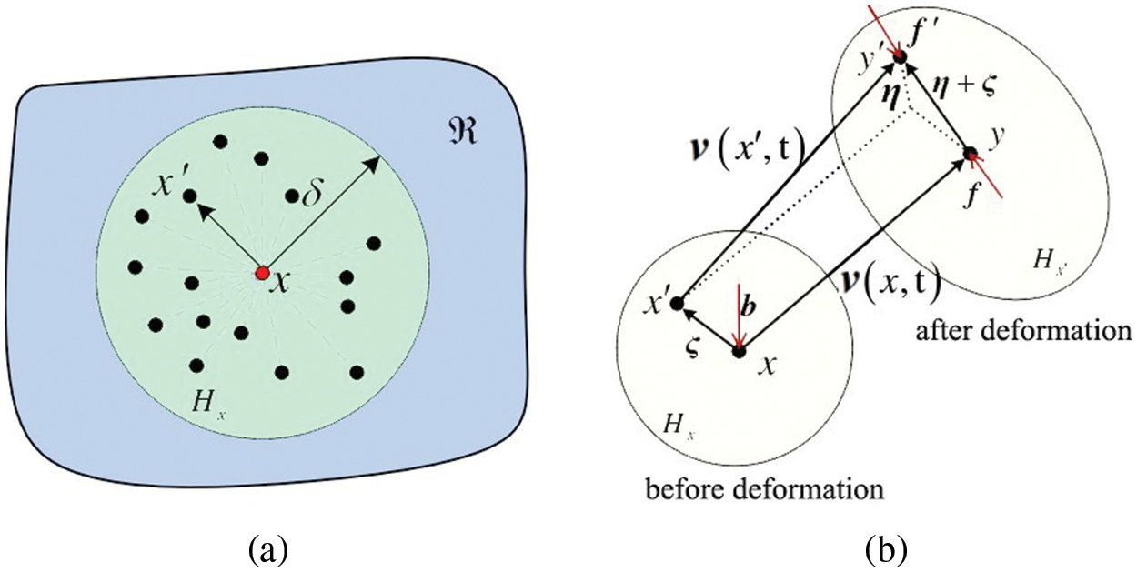
Figure 1: The interaction of material points in bond-based PD theory

ζ=x′−x.(1)

In the current configuration following deformation, the relative displacement vectors η of the two material locations are expressed as follows:

η=ν(x′,t)−ν(x,t).(2)

where ν(x′,t) and ν(x,t) are the displacement field vectors of material points x′ and x at t time, respectively. Then, the relative position vector of the two material points in the current configuration is:

y′−y=ζ+η.(3)

According to Newton’s second law, the equation of motion of any material point x in the horizon at t time is as follows:

ρν..(x,t)=∫Hxf(ν(x′,t)−ν(x,t),x′−x)dVx′+b(x,t).(4)

where ρ is the density of the material, b is the external force or the density of physical force, ν.. is the acceleration, Vx′ is the volume of the material point x′, and f is the pairwise force vector per unit volume squared that x′ exerts on x. In the current reference configuration, the direction of the PD bond force is parallel to the direction of the relative position vector of these material points, and there are:

f=f(ν(x′,t)−ν(x,t),x′−x)=f(η,ζ)=0∀|ζ|>δ.(5)

The PD force f satisfies the law of linear conservation of momentum: the acting force and the reaction force between two material points are equal, and the direction is opposite, that is, the linear allowable condition in PD theory:

f(−η,−ζ)=−f(η,ζ)∀η,ζ.(6)

In addition, it satisfies the law of conservation of angular momentum:

(η+ζ)×f(η,ζ)=0∀η,ζ.(7)

PD bond forces can be described in the following forms for elastic isotropic materials:

f=c(ζ)s(η,ζ)ζ+η|ζ+η|.(8)

where c(ζ) is the micro-modulus, a constitutive parameter of the PD model known as bond stiffness, and s(η,ζ) represents the bond tension.

The strain energy density WPD(x) obtained by PD theory equals the strain energy density WCCM(x) obtained by classical continuum mechanics theory under simple loading, allowing the relationship between bond stiffness c and material constant to be determined. The link between PD parameters and traditional mechanical parameters is shown by Silling [12] using strain energy density and energy release rate experiments.

c=18kπδ4(9)

where k is the bulk modulus of the material, the bulk modulus of the isotropic material is k=E3(1−2v), and δ is the horizon size.

The elongation s(η,ζ) of the bond can be expressed as follows when using the maximum tensile failure criterion to determine whether the bond is broken or not:

s=|ζ+η|−|ζ||ζ|.(10)

When the bond is pulled, the value of s is positive, and when compressed, it is negative, which is quite similar to the definition of strain in material mechanics. |ζ| is the original length of the bond in the reference configuration and |ζ+η| is the deformed length of the bond in the current reference configuration.

2.2 Damage Criterion

The critical tensile value of the bond is s0. When the bond elongation between any two material points surpasses this critical value, the interaction between the two material points ceases instantaneously, introducing damage into the constitutive model of PD theory through the bond fracture. The micro-crack will be formed when the bond fractures in the model. The macroscopic crack is the discontinuous space generated by broken bonds when a given number of bonds have been disrupted. The break of the bond is connected with the introduction of the failure parameter μ(t,ζ), therefore the pairwise force of PD can be represented as follows:

f=g(s)μ(t,ζ).(11)

where g(s)=cs (c is a constant) is a linear scalar function with respect to bond elongation. μ(t,ζ) is a historically dependent scalar function used to describe the destruction of bonds between material points. The function value of 1 means that the bond has not been broken, whereas the function value of 0 means that the bond has been broken, as seen below:

μ(t,ζ)={1 if s<s00 otherwise .(12)

The critical tensile s0 of isotropic materials can be calculated using the macroscopically determined fracture energy G0. The critical tensile values of prototype microelastic brittle (PMB) materials are as follows:

s0=10G0πcδ5=5G09kδ.(13)

As a result, Fig. 2 depicts the PD constitutive relationship of PMB material (the relationship between bond force f and bond elongation s).

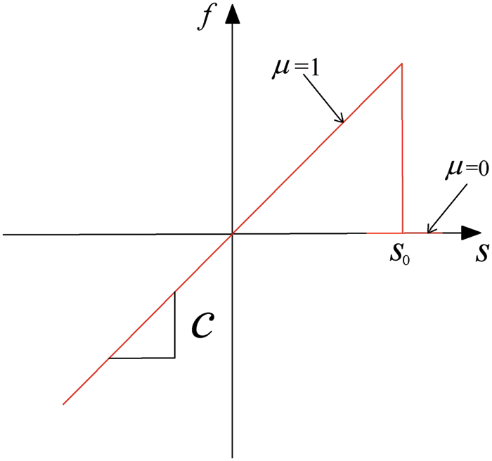
Figure 2: The relationship between bond force f and bond stretch s of PMB materials

The variable φ(x,t) expresses the local damage degree of a material point x in an object at t time. According to the definition of “bond” failure in PD theory, the value of this variable can be defined as the ratio of the number of broken bonds to all bonds in all material points interacting with material point x in the horizon Hx:

φ(x,t)=1−∫Hxμ(t,ζ)dVx′∫HxdVx′.(14)

The variable has a range of values from 0 to 1, with 1 indicating that the bond that initially interacts with the material point is totally broken and 0 indicating that the bond is completely intact. The local damage degree of a material point is an essential index for determining the likelihood of cracks occurring in the object. In the beginning, a material point interacts with all the material points on its horizon, so its local damage value is 0. About half of the interaction is terminated by the formation of cracks. The value of local damage is 0.5, indicating that a crack may form, as shown in Fig. 3. As a result, the constitutive relation of the PD model already incorporates the description of damage and fracture. No additional crack propagation criteria are required. With the increase of the load on the structure, the whole process of crack start and propagation in the model can be simulated spontaneously by breaking the bonds in the horizon of the material point one by one.

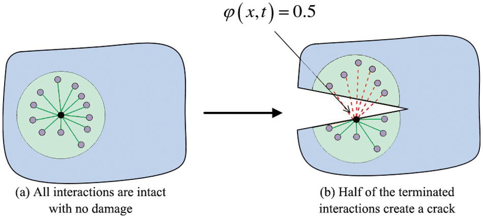
Figure 3: Schematic diagram of crack formation

2.3 Numerical Method

The research body must be uniformly dispersed into material points with a specified volume when using the numerical approach to solve the equation of motion in the form of PD integral, and the mass of the material point must be concentrated in its midway. PD discrete equations of motion can be written as follows:

ρν¨in=∑pf(νpn−νin,xp−xi)Vp+bn.(15)

where ρ is the material density, ν¨in is the acceleration of the material point i, n is the number of time steps, the subscript represents the material point number, νin=ν(xi,tn) represents the displacement of the material point i at n time steps, Vp is the volume of point p within the horizon of material point i.

The volume of some material points is completely included in the horizon radius of a certain material point i during the spatial discretization process in the theory of PD. However, the volume of other material points is not completely included. As a result, the accuracy of the numerical simulation during the calculation will be affected. Therefore, the volume of the specific material point j needs to be corrected.

Vj={Δx3(|ξ|<δ−0.5Δx)[(δ+0.5Δx−|ξ|)/Δx]Δx3(δ−0.5Δx<|ξ|<δ−0.5Δx)0 otherwise (16)

where Δx is the spacing between two neighboring material points, δ is the horizon range of a certain material point i, and Vj is the volume of the specific material point j.

On the left side of Eq. (15), the acceleration can be stated as an explicit central difference.

ν¨in=νin+1−2νin+νin−1Δt2(17)

Silling et al. [14] investigated the effect of time step on result convergence and proposed convergence conditions.

νtn=λne(κi−1)(18)

where n is the time step, κ represents a real number, and λ represents a complex number. In order to achieve the stability requirements, all κ values must be satisfied to avoid the infinite growth of stress waves.

Because the central difference method is an explicit integration algorithm with conditional convergence, the time step Δt must satisfy the following conditions for the algorithm to be stable.

Δt<2ρ∑j=1N⁡c‖xj−xi‖Vp(19)

where N is the total number of material points within the horizon of the material point xi. Vp and c are the volume and micro-modulus of other material points, respectively, on the horizon of the material point p.

In this paper, the adaptive dynamic relaxation (ADR) method is used to add damping to the equation of motion to solve static or quasi-static problems. Therefore, Eq. (15) can be turned into an ordinary differential equation by adding a damping system:

DV¨(X,t)+ηDV˙(X,t)=F(V,V′,X,X′)(20)

where D is the diagonal density matrix, and η is the damping coefficient. X and V are the initial position and displacement vector of discrete material points, respectively, and they can be expressed as:

XT={x1,x2,x3,…,xM}(21)

VT={v(x1,t),v(x2,t),v(x3,t),…,v(xM,t)}(22)

where M is the number of all material points in the structure, F is the sum of all internal and external forces of the structure, and the component i in the F vector can be expressed as:

Fi=∑f(νp−νi,xp−xi)Vp+bi(23)

The displacement and velocity at the next iterative time step can be stated as follows using the revealed central difference method:

V˙t+1/2Δt=((2−ηt)V˙t−1/2Δt+2ΔtD−1Ft(2+ηtΔt)(24)

Vt+Δt=Vt+ΔtV˙t+1/2Δt(25)

where n denotes the number of iterations, the number of time iteration steps is commonly set to 1 (Δt=1) when using the ADR approach. Please refer to [28] for selecting the diagonal components of the density matrix D.

The algorithm flow chart (Fig. 4) for applying PD theory in numerical simulation is shown below to understand the numerical calculation process better.

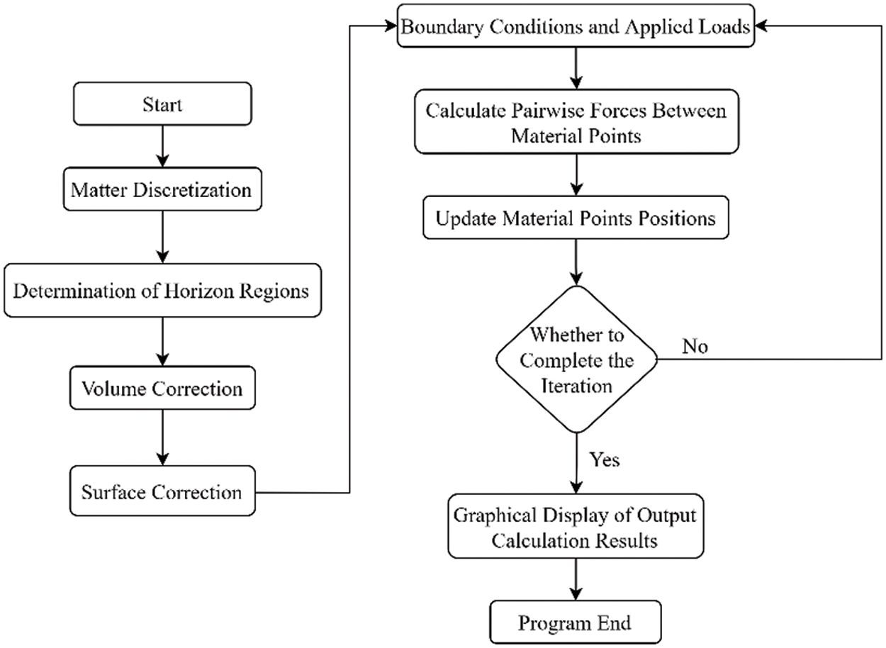
Figure 4: The PD algorithm flow chart

The program’s pre-treatment part is the discretization of the material point, the determination of the horizon region, and the volume and surface correction. If there is a crack in the model’s initial state, it is necessary to pre-construct the crack on the model so that all the bonds passing through the crack surface are broken. Suppose the elongation of the bond exceeds the critical elongation when calculating the pairwise force to judge the elongation of the bond. In that case, the bond must be marked as having an irreversible fracture and will no longer participate in the computation of the subsequent pairwise force. After the pairwise force has been determined, the material point’s acceleration needs to be estimated based on the force, and the velocity and displacement of the point can be derived using the central difference algorithm to update the position of the material point.

3  Feasibility Study on Peridynamics of Lining Cracks

Japan Tunnel Research Institute [29] conducted an indoor 1:1 liner model test. The load and surrounding rock resistance were applied by 34 jacks placed on the outer surface of the lining. The crack propagation under the action of concentrated load on the lining arch, voids behind the lining and unstable rock strata are studied, respectively (Fig. 5). In order to verify the applicability of PD simulation of lining crack propagation process and law, the fractures in the tunnel lining are numerically analyzed using the above prototype microelastic brittle material model and the adaptive dynamic relaxation approach. This paper establishes a concentrated load model of lining vault. Compared to the prototype test described above, two failure possibilities are primarily considered: the concrete reaches ultimate compressive strength and collapses, and the concrete reaches ultimate tensile strength and cracks. The fracture energy is 80N/m, Young’s modulus is 23.47 GPa and, the Poisson ratio is 0.25, the density is 2,400kg/m3. For detailed simulation parameters, please refer to the literature [30]. The criterion for crack propagation uses the strain energy density factor, which is based on the notion of equivalent strain energy density.

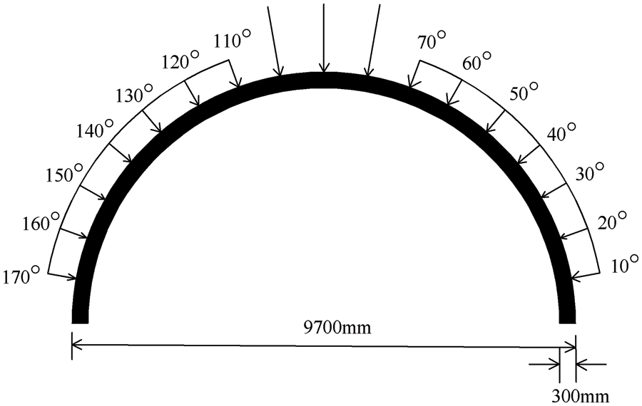
Figure 5: Schematic diagram of prototype experimental tunnel model

3.1 The Effect of Material Point Spacing on Cracks

In order to study the effect of material points spacing in tunnel crack simulation, four numerical modes with the material point spacing of Δx=L/200, Δx=L/300, Δx=L/400, and Δx=L/500 were selected, where L=9.7m. Horizon size is specified as δ=3Δx. The cracks under different material point spacing are shown in Fig. 6. The characteristics of tunnel cracks in the four numerical models are similar. As the number of material points increases, the crack distribution becomes clearer, and the contour becomes smoother. It illustrates that when the material point spacing lowers, the PD model’s accuracy improves, but it cannot grow indefinitely, which is consistent with the PD theory’s δ-convergence law. The material point spacing can be taken as Δx=L/400, which fits the simulation requirements, considering the computation cost and accuracy.

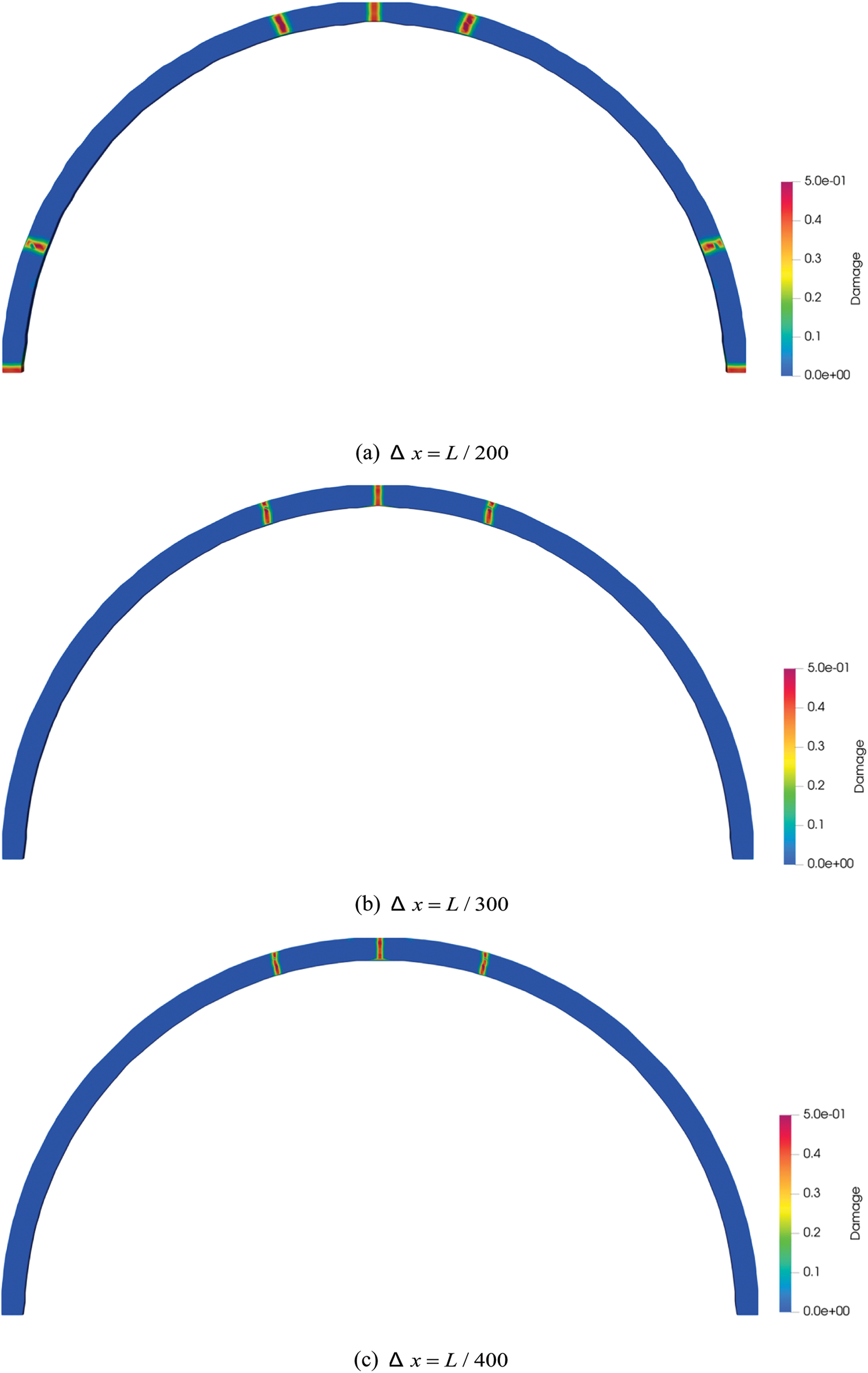
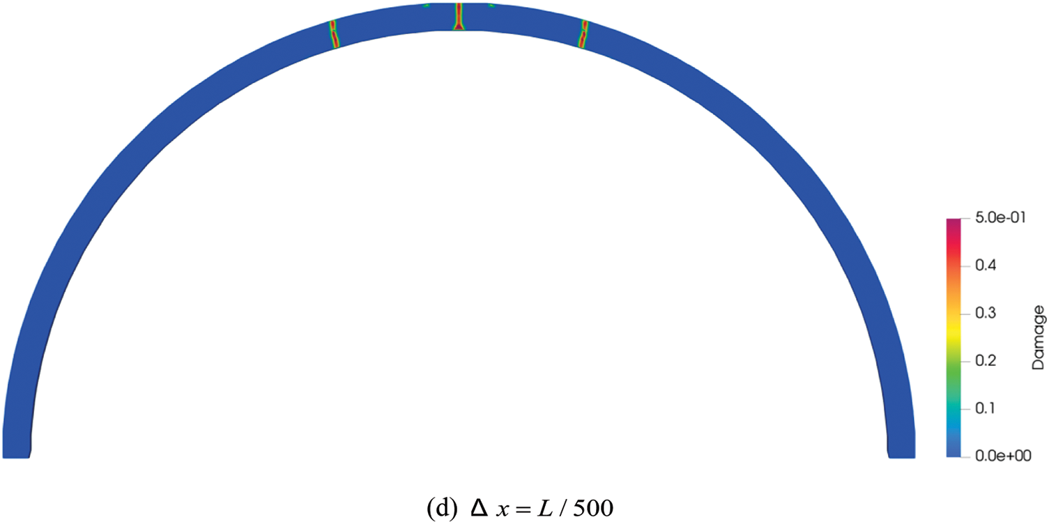
Figure 6: The distribution characteristics of cracks at different sizes of material point spacing

3.2 The Influence of Horizon Size on Cracks

Four numerical simulations with horizon size of δ=2Δx, δ=3Δx, δ=4Δx, and δ=5Δx were undertaken to investigate the m-convergence features of the PD. The material point spacing is specified as Δx=L/400. The distribution features of fractures at various horizon sizes are shown in Fig. 7. Under different horizon sizes, cracks’ distribution places and forms are comparable. However, when the horizon size is too small or too large, some calculation mistakes appear in the simulation results. This is because the smaller horizon size cannot capture the fracture propagation behavior. The horizon size can be set to δ=3Δx, which fits the present numerical simulation requirements.

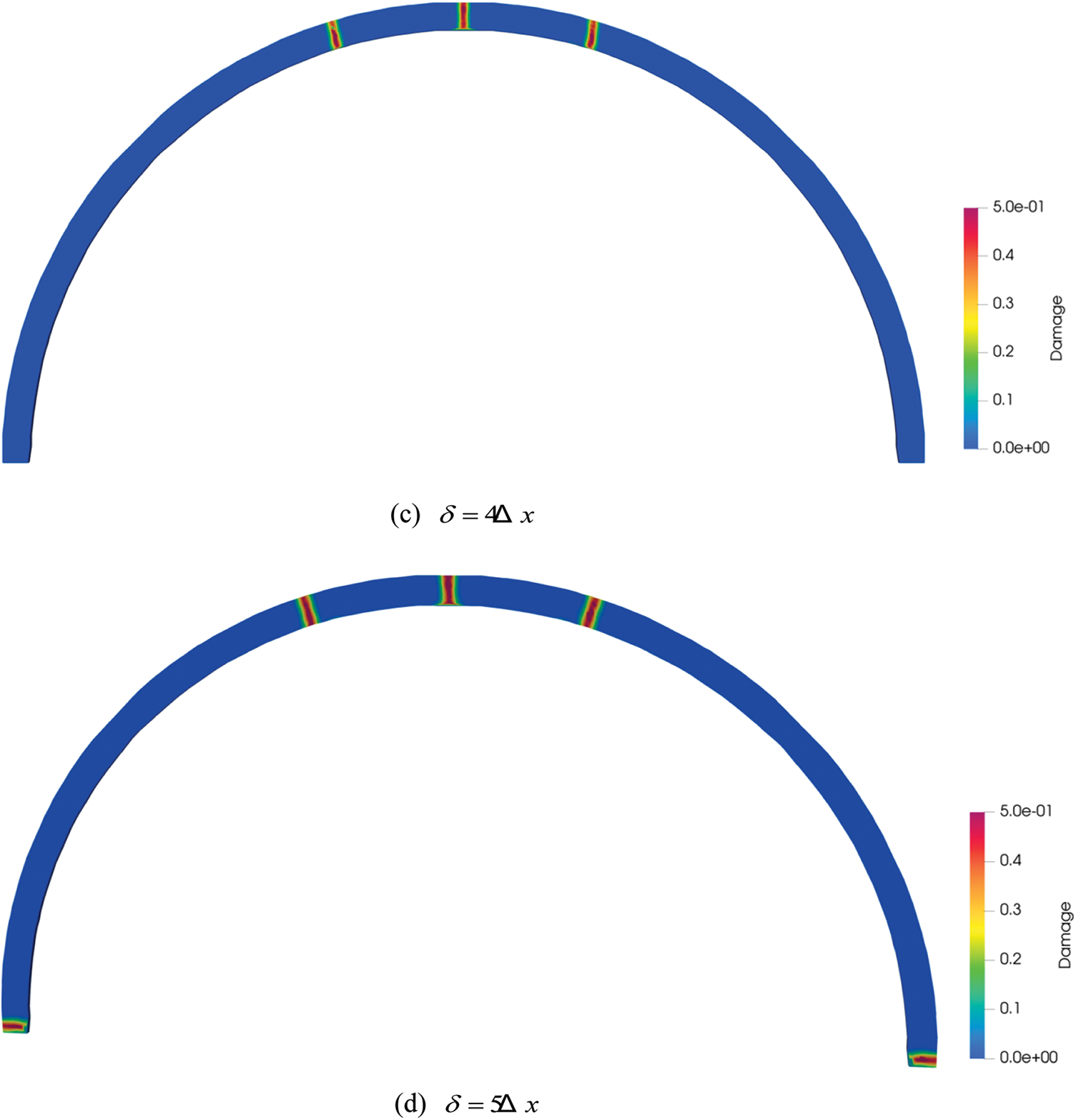
Figure 7: The distribution characteristics of cracks at different horizon sizes

3.3 Verification

The crack distribution state diagrams derived from the indoor prototype test and the load-vault displacement comparison curves are depicted in Figs. 8 and 9. The PD method in Fig. 9 adopts the horizon size δ=3Δx and the material point spacing Δx=L/400.

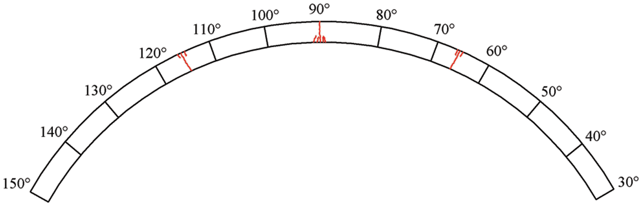
Figure 8: Prototype experimental crack expansion diagram

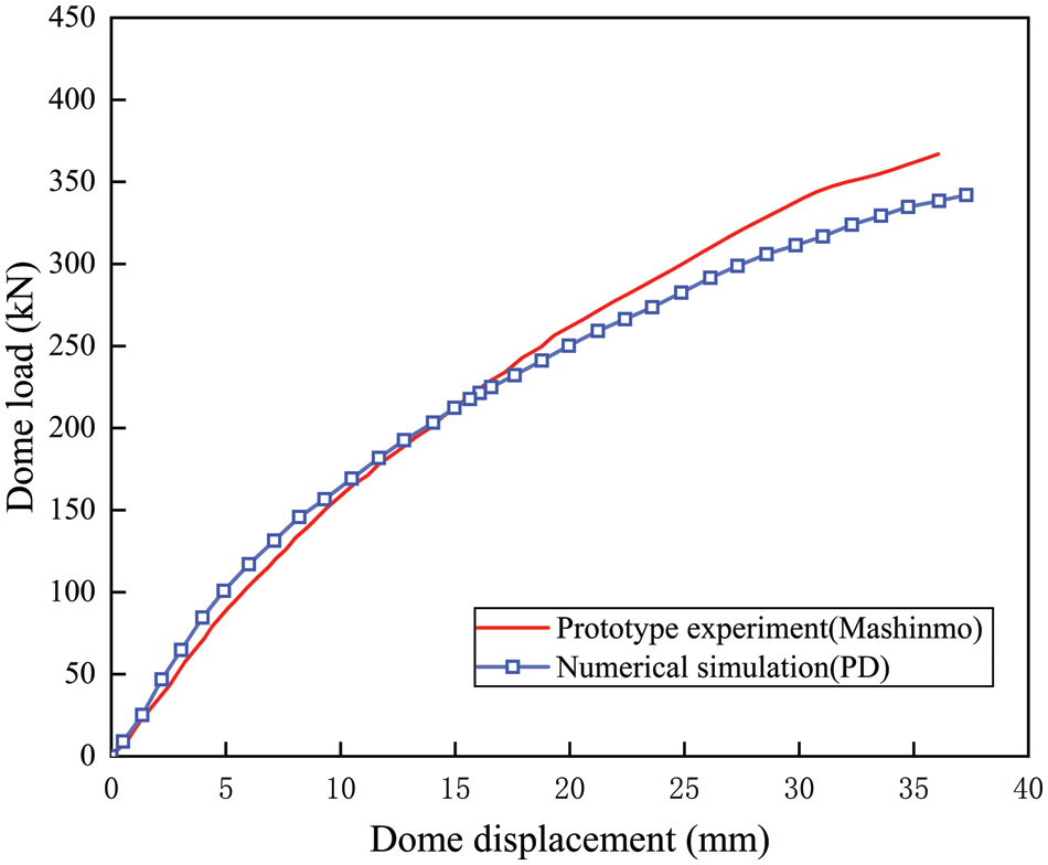
Figure 9: Comparison of load-displacement curves at vault between numerical modeling and laboratory tests

The results of the comparison show that the load-vault displacement curves of the two have the same trend, the curve fitting is good, the vault displacement generated by the early loading of the numerical simulation is larger than that of the prototype test, and the vault displacement generated by the later loading of the numerical simulation is smaller than that of the prototype test. According to the prototype test process analysis, the inhomogeneity of the external force simulated by the jack and the resistance of the surrounding rock is the main explanation for the differences in the results. The crack distribution state diagram indicates that the two results are essentially consistent in terms of crack location and distribution. As a result, the PD approach can be used to replicate the progressive cracking process of lining cracks.

4  Peridynamic Analysis of the Main Influencing Factors of Cracking

The results of the on-the-spot investigation on the crack diseases of 48 highway tunnels in the Zhejiang region in [31] show that the proportion of cracks in the vault, arch waist, and side wall is 42.27%, 27.08%, and 30.65%, respectively. The vault, which accounts for 64.92% of longitudinal cracks, is followed by the arch waist, which accounts for 27.30% of longitudinal cracks. The numerical simulation of progressive cracking of lining structures is carried out using the tunnel maintenance and improvement project as the main example. The relevant parameters of the model are as follows: the radius of the tunnel is 9,700 mm, the thickness of the lining is 300 mm thick C30 concrete, the fracture energy is 80N/m, the Young modulus is 20.7 GPa, the Poisson ratio is 0.25, the density is 2,420kg/m3, and the surrounding rock pressure is 20 kPa.The fractures in the tunnel lining are numerically analyzed using the prototype above microelastic brittle material model and the adaptive dynamic relaxation approach. The horizon size δ = 3Δx can produce a decent simulation outcome in macro-scale simulation. A too-small selection of the horizon size will lead to a grid effect; too large will lead to the diffusion of stress waves and increase the calculation cost. After careful consideration, the horizon size is specified as δ = 3.015Δx, which considers both the calculation efficiency and the crack propagation accuracy. According to the convergence study above, the material point spacing is selected Δx = L/400.

4.1 Local Bias Pressure

The significant asymmetry of tunnel surrounding rock pressure leads to the eccentric pressure on the lining structure, divided into two types: topographic bias pressure and local bias pressure [32–34]. The paper only studies the crack propagation under the action of local bias pressure in the range of 30° arch waists (80°~50°, the right baseline of the tunnel is 0° and rotates counterclockwise) because of the actual bias pressure position of the project. Fig. 10 is a schematic diagram for the calculation of local bias pressure. Based on the original confining pressure load, the load of the bias part is gradually increased. The PD method is used to compare and analyze three working conditions: the range of the bias pressure is 10° (located between 80° and 70° of the arch waist), 20° (located between 80° and 60° of the arch waist) and 30° (located between 80° and 50° of the arch waist).

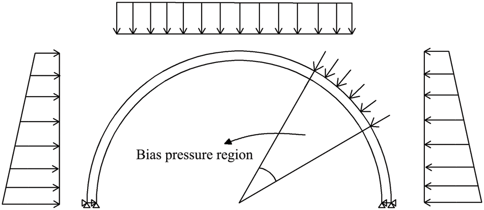
Figure 10: Calculation of bias pressure

When the load reaches a certain value, tension cracks appear on the inner surface of the lining arch waist. As the bias load increases, the tension cracks on the inner surface of the lining continue to expand, while pressure cracks appear on the outer surface of the lining near the 60° arch waists. The crack distribution law is shown in Fig. 11. The local magnification diagram shows the propagation of the corresponding cracks in the total time of 1 ms. For the convenience of comparison, the maximum crack damage factor of the local magnification map is 0.5. The maximum value of the crack damage factor increases with the increase of the bias pressure range. Tensile cracks form first on the inner surface of the lining when the range of local bias pressure is small (10° working condition). Then, the cracks on the inner surface continue to expand, and the effective bearing part gradually declines. When the range of local bias pressure reaches a certain value (20°, 30°), wider tensile cracks emerge on the lining’s inner surface. The lining’s failure mode swiftly shifts to overall failure produced by compression of the outer surface. Fig. 11c shows a type ‘I’ pressure crack on the arch waist’s outer surface during 236 μs.

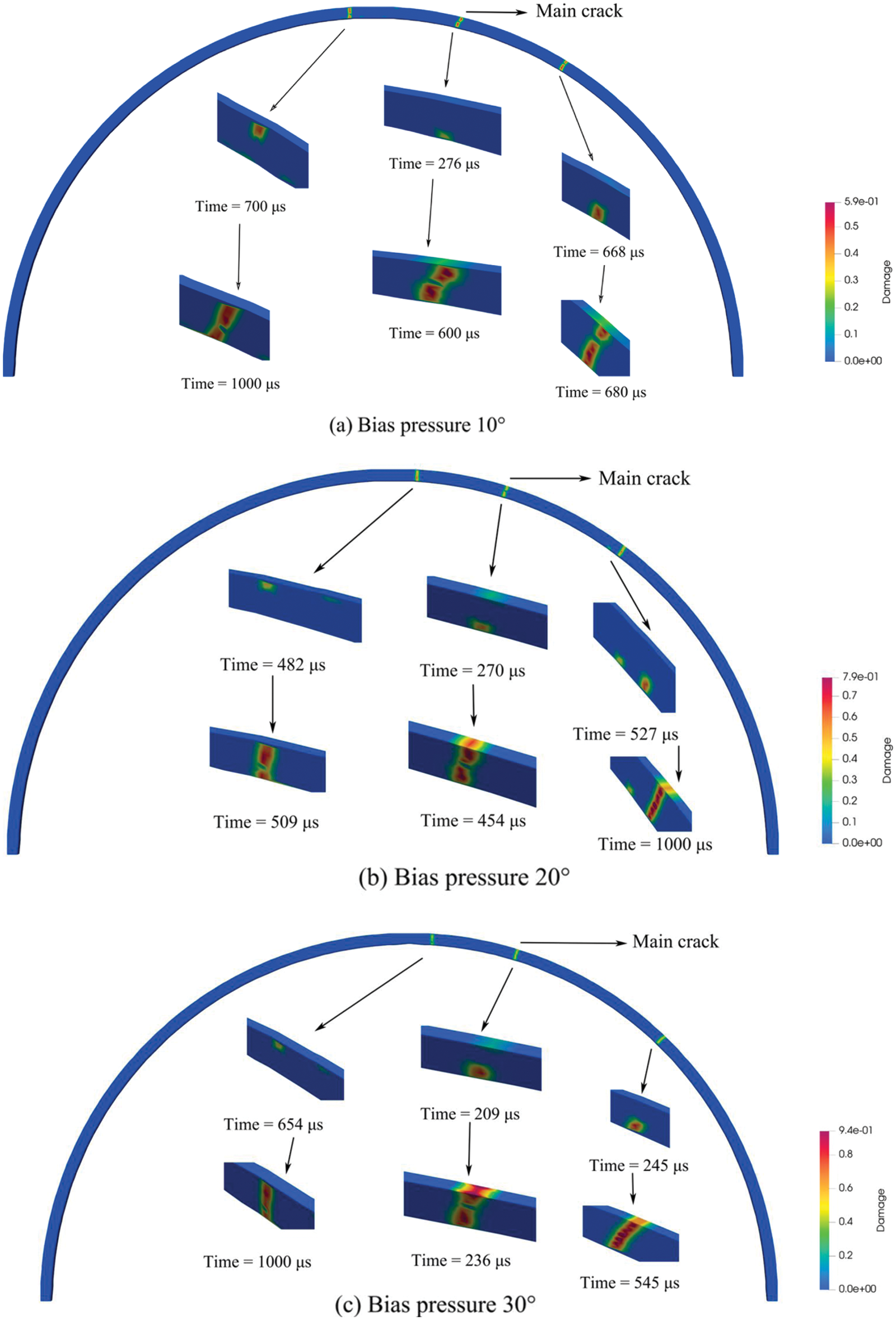
Figure 11: Fracture distribution state diagram under bias pressure

Fig. 12 shows the change in crack depth over time induced by tension on the inner surface and compression on the outside surface of the arch waist under three bias pressure conditions. The larger the bias pressure angle, the earlier the crack forms, and the tension crack appears before the compression crack, as illustrated in the image. When the bias pressure angle is 30°, the extended depth of the tensile fracture on the inner surface after failure is obviously less than 10 degrees, indicating a structural geometric instability failure tendency.

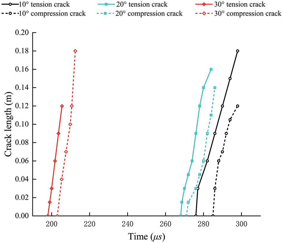
Figure 12: Main crack (inner surface tension crack and external surface compression crack) advance curves with three different bias pressure angles

Considering the paper’s length and the similarity of the stress field diagrams for different bias angles, we chose a bias angle of 10 degrees as an example. The normal stress field predicted by the PD method is displayed in Fig. 13.

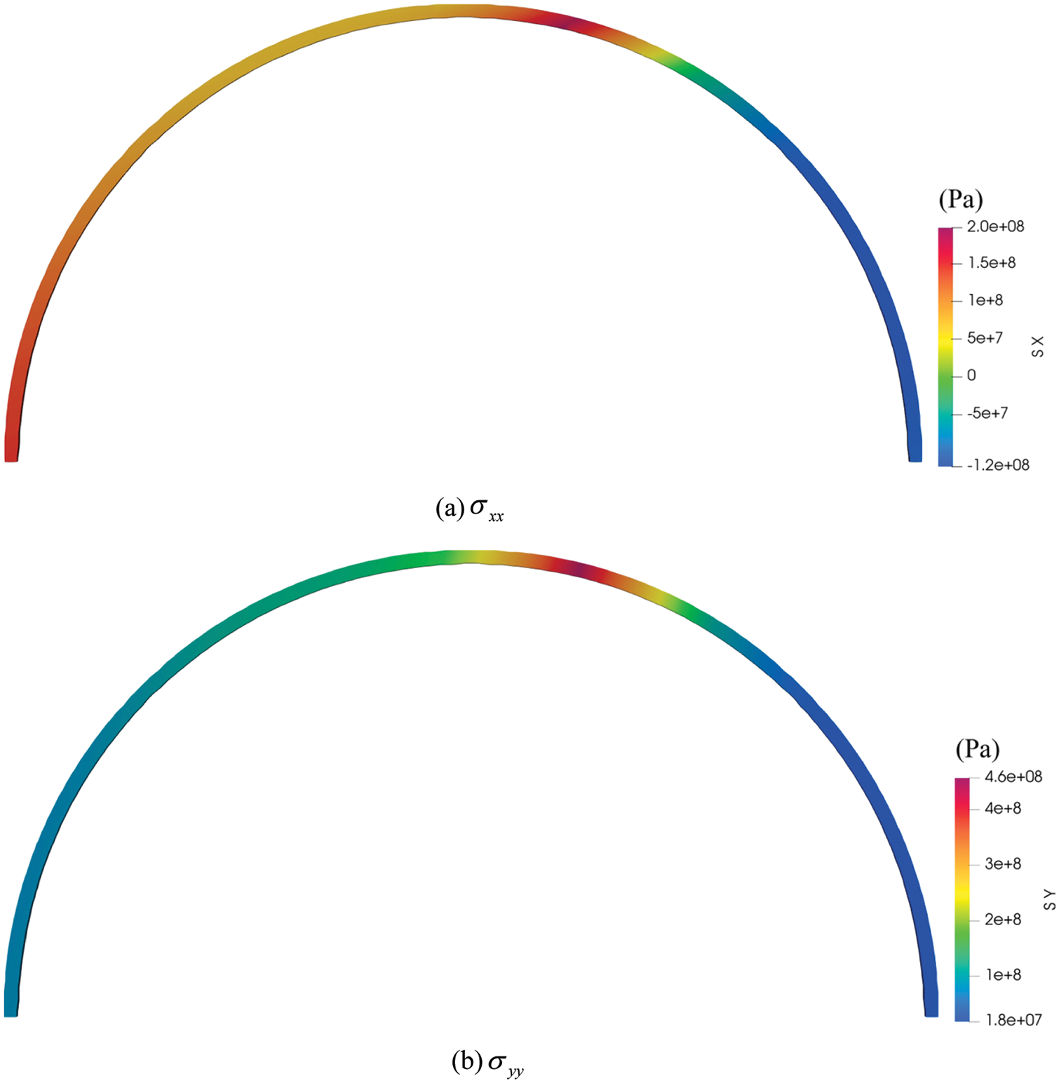
Figure 13: The normal stress field diagrams of lining under bias pressure angle of 10 degree

4.2 Lining Thickness

In order to analyze the influence of lining thickness on lining crack propagation under local bias pressure, the outer diameter of the tunnel is unchanged, the lining thickness is 500 mm, and the loading confining pressure and bias pressure are consistent with those in Section 4.1. Fig. 14 shows the distribution of lining cracks when the 500 mm thickness lining model is destroyed. The earliest cracking portions of the two structures are similar during continuous loading. The cracks are mostly open when the 300 mm thickness lining model is damaged. When penetrating cracks appear in the arch waist, new cracks arise on both sides of the current portion. However, there is no penetrating crack in the 500 mm thickness lining model under 10° and 20° bias pressure conditions. Although the penetrating crack is produced under the condition of 30° bias pressure, the relative depth of the new right crack is obviously smaller than that of the 300 mm lining.

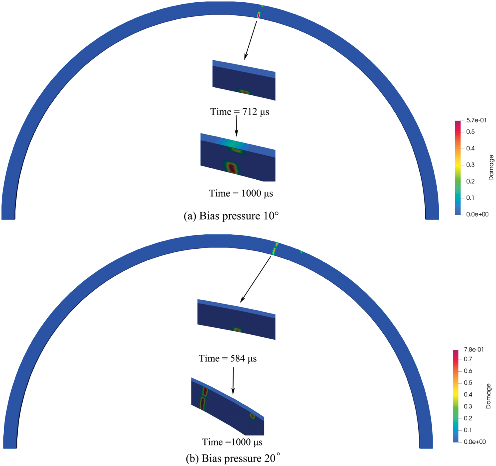
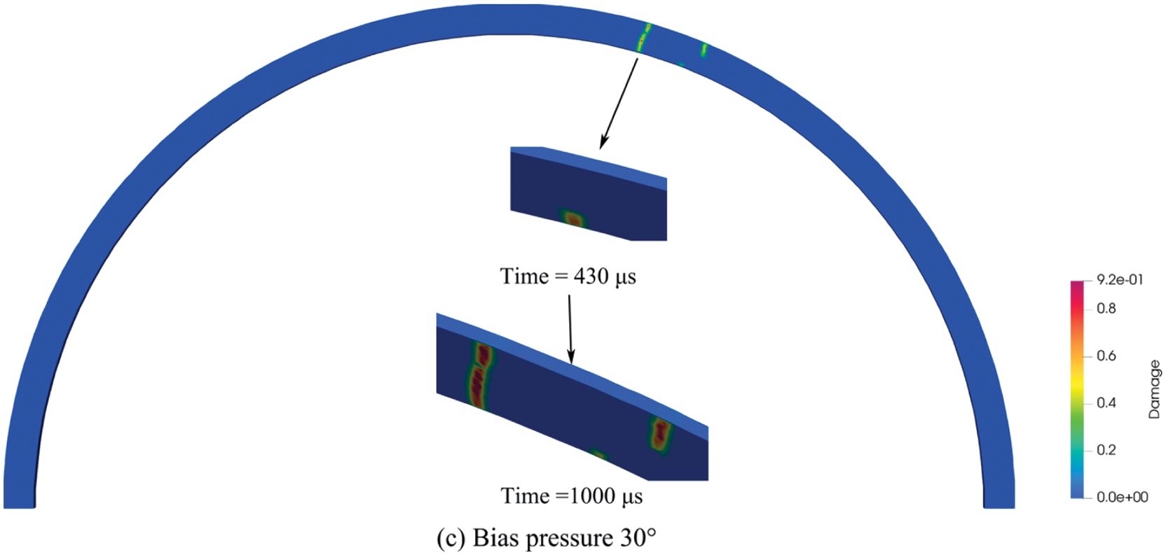
Figure 14: State diagram of crack distribution in different lining thicknesses

The relative depth is clearer to indicate the fracture propagation depth due to the different thicknesses of the lining. Fig. 15 depicts the main crack propagation on the inner surface of the arch waist with different lining thicknesses under three kinds of bias pressure. At 10° bias pressure, the crack propagation of 300 mm lining is much larger than that of 500 mm, due to the penetration crack of 300 mm lining. The 20° bias pressure is similar to the 10° bias pressure. Both types of lining thickness have penetrating cracks under 30° bias pressure. However, the crack propagation of the 500 mm lining is much larger than that of the 300 mm, and the crack appears later, indicating that the lining damage of the 500 mm lining thickness is primarily tensile crack propagation.

Figure 15: Main crack (inner surface tension crack) advances curves in different lining thicknesses

Similarly, the normal stress diagram of the lining with increased thickness is shown in Fig. 16 at a bias pressure angle of 10°.

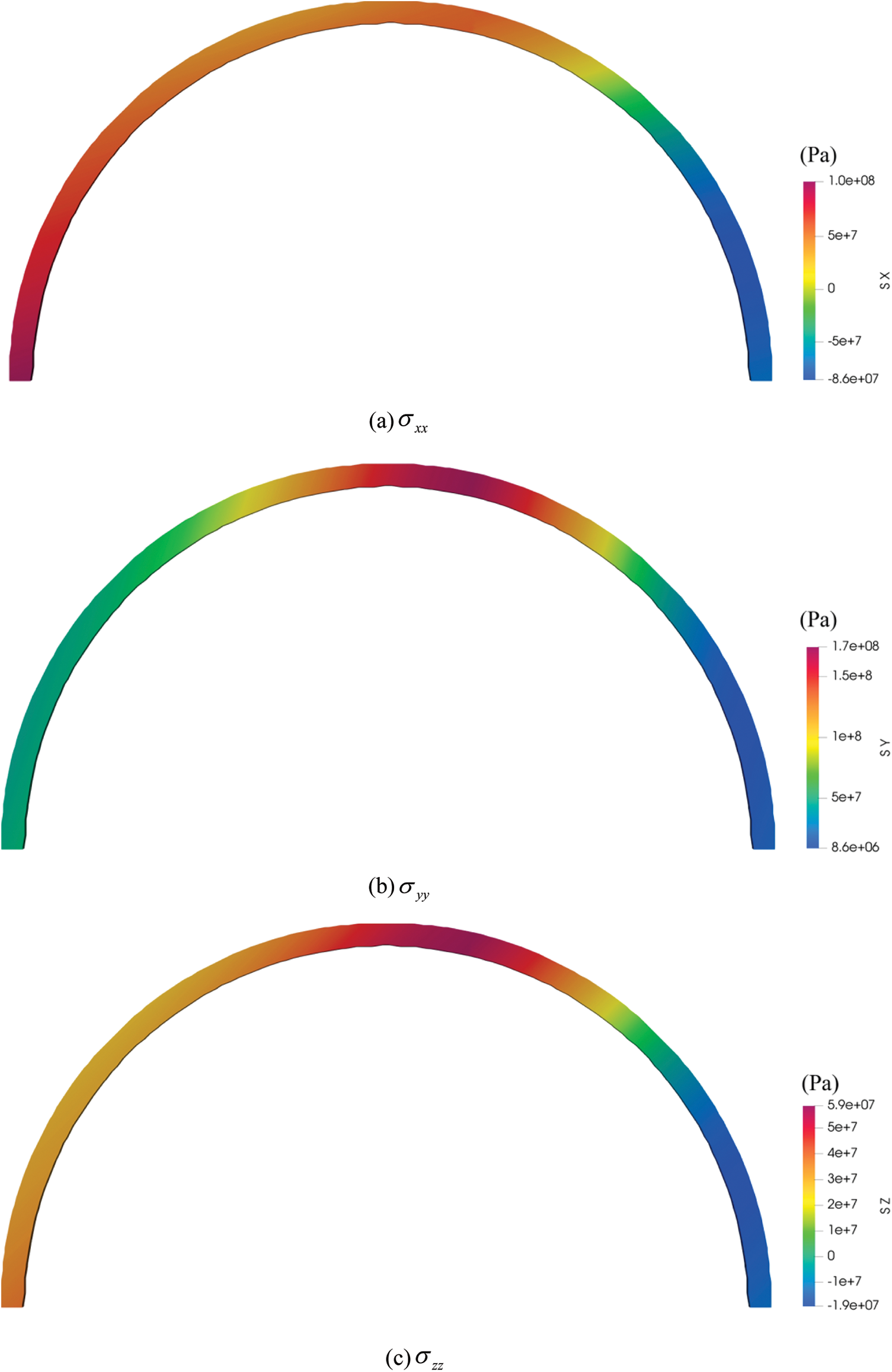
Figure 16: The normal stress field diagrams of lining with increased thickness under a bias pressure angle of 10 degree

4.3 Damaged Lining

Cracks often accompany the lining, so it is necessary to study the existing cracks. In this section, the inner surface of the lining is preset with 90° vertical compression cracks, 30° symmetrical tension cracks, and 60° symmetrical tension cracks with a crack depth of 100 mm. Fig. 17 displays the fracture propagation under the three working conditions. Only half of the lining is taken because the crack is symmetrically distributed. A compression crack with a vertical angle of 90 degrees is shown in Fig. 17a. A tensile crack appears at the preset crack’s location before the compressive crack begins to propagate, showing that tensile stress is the primary cause of lining failure and that the initial crack initiation did not occur at the preset crack’s tip. After the vertical crack propagates for a while, a new crack appears at 60° on the left side of the arch waist, indicating that the left side of the arch waist is also a dangerous position under the influence of the preset crack. For the tensile cracks preset at the arch waist of 30° (Fig. 17b) and 60° (Fig. 17c), the positions of the new tensile cracks around the preset cracks are similar, so more attention should be paid to the lining treatment.

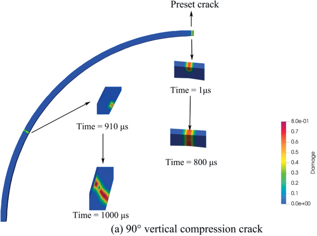
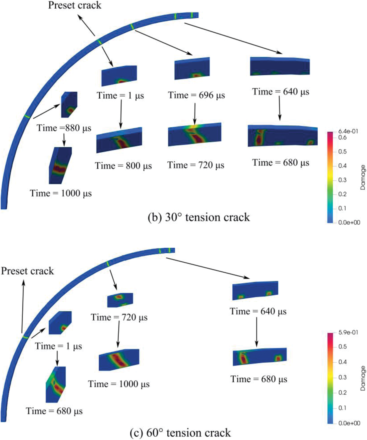
Figure 17: Crack distribution state diagram of different preset crack positions

Fig. 18 shows the crack propagation depth on the inner surface of the preset crack as a function of time in three different working situations. The working condition of 90° is a preset pressure crack, so the tensile crack on the inner surface begins to expand from 0, and both 30° and 60° begin to expand from the depth of 0.1 m. The propagation depth of inner surface crack under 60° condition is lower than that under 30° condition, which indicates that the failure mode of lining under 60° condition changes to outer surface pressure faster than that under 30° condition. However, the 30° condition damage factor is higher than that of the 60° condition, and the crack propagation slope is steeper, implying a faster propagation speed.

Figure 18: Preset crack (inner surface tension crack) advances curves in different positions

The normal stress diagram of the lining with preset cracks in different positions is shown in Figs. 19–21.

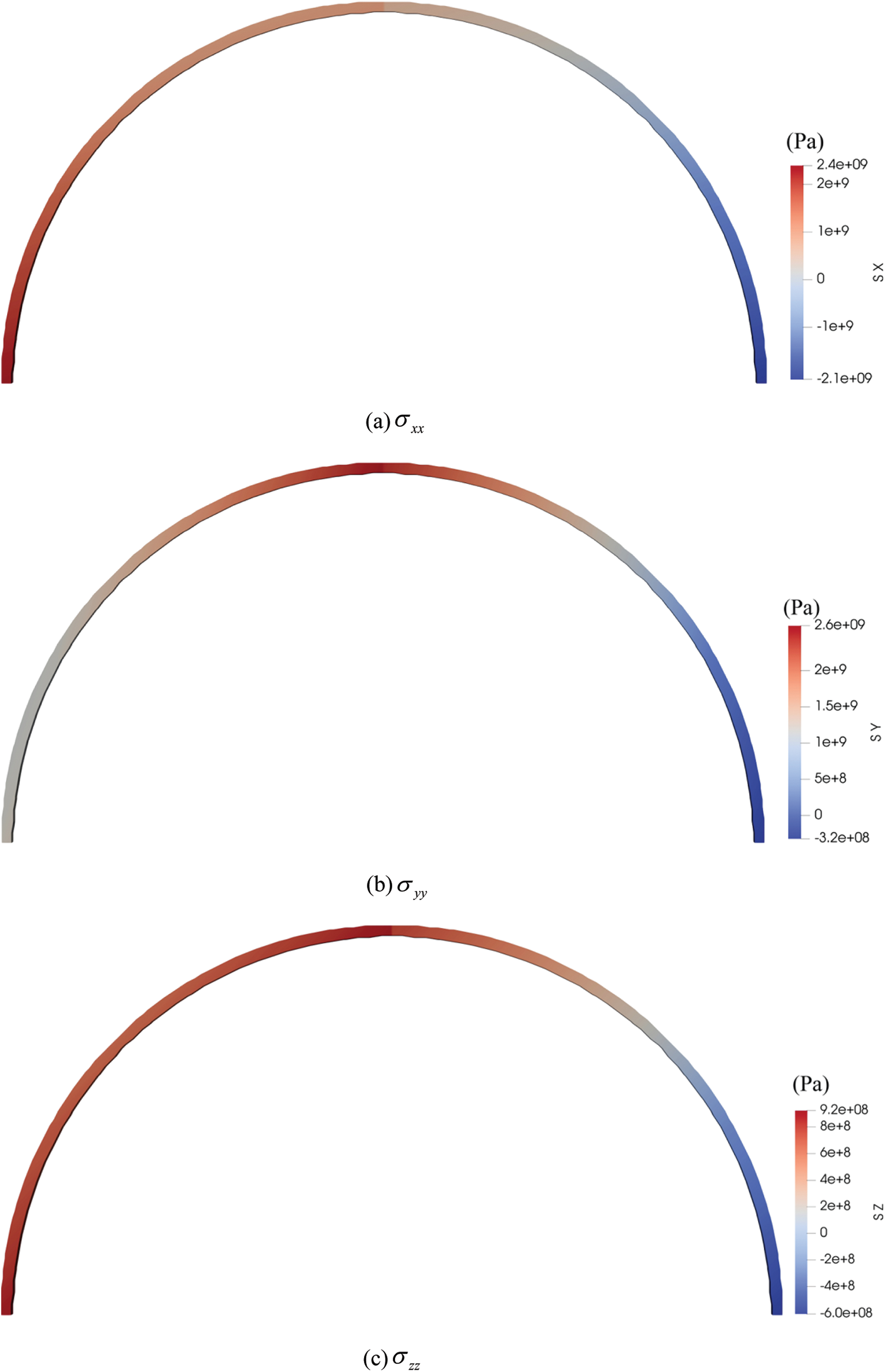
Figure 19: The normal stress field diagrams of lining with 90° vertical compression crack

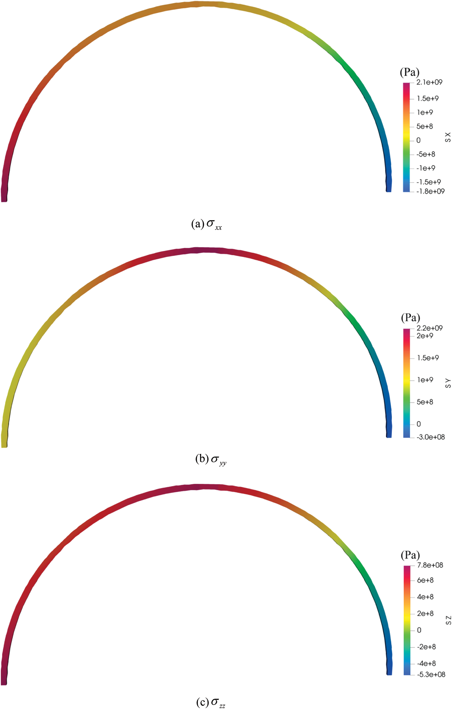
Figure 20: The normal stress field diagrams of lining with a 30° tension crack

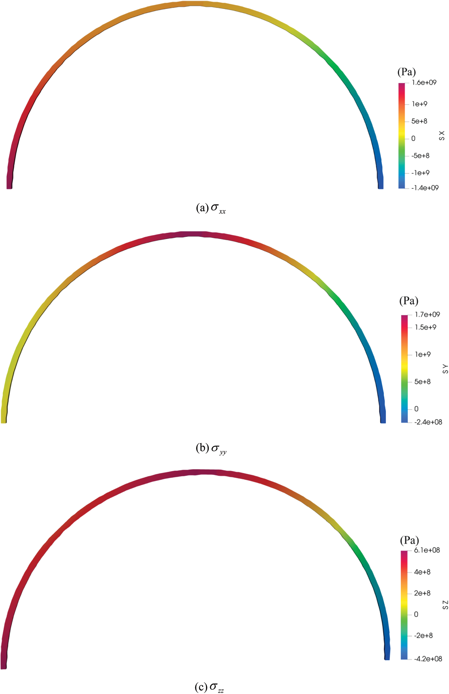
Figure 21: The normal stress field diagrams of lining with 60° tension crack

4.4 Lining Section Shapes

This section mainly studies the propagation of cracks in the lining with the tunnel invert under bias pressure (the data are the same as in Section 4.1). It can be seen from Fig. 22 that the position and shape of the generated cracks are almost the same as those in Section 4.1. A new crack is generated at the junction of the inverted arch and the upper semicircle of the tunnel lining, but there is no crack at the inverted arch.

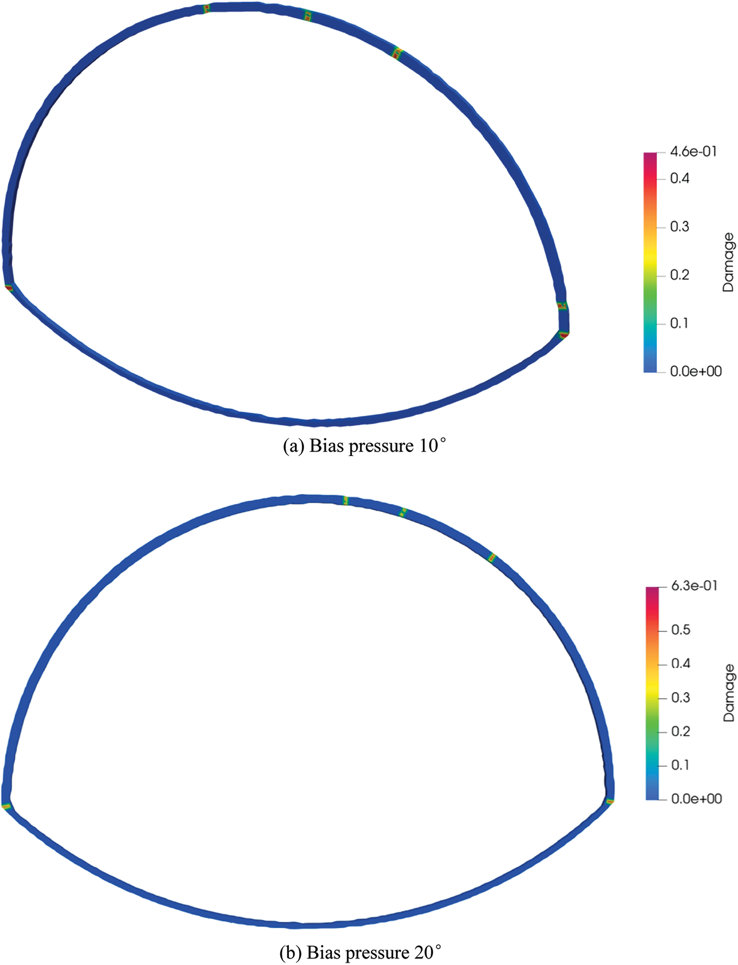
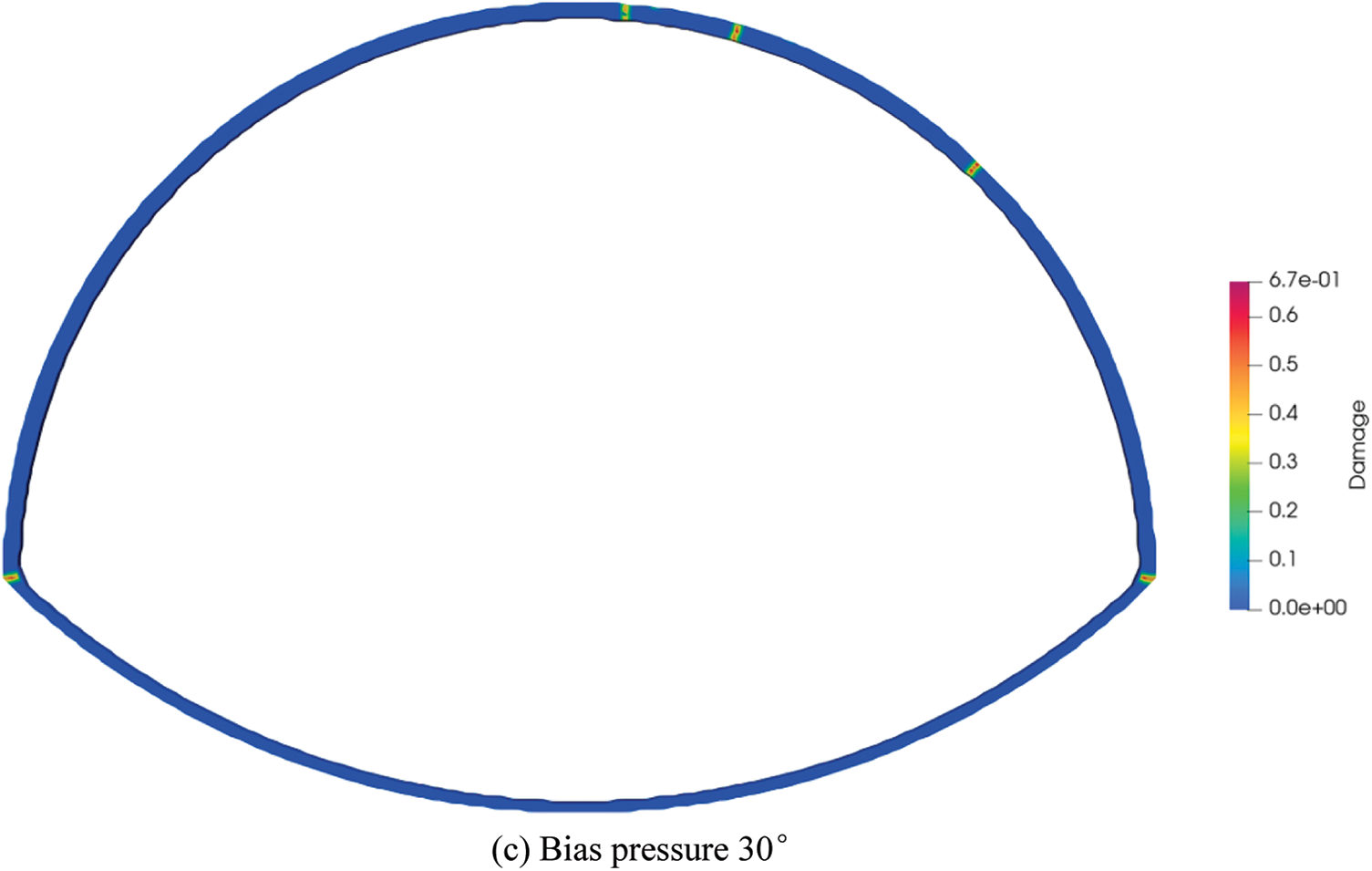
Figure 22: Crack distribution state diagram of the lining with tunnel invert

Similarly, the normal stress diagram of the lining with tunnel invert is shown in Fig. 23 at a bias pressure angle of 10°.

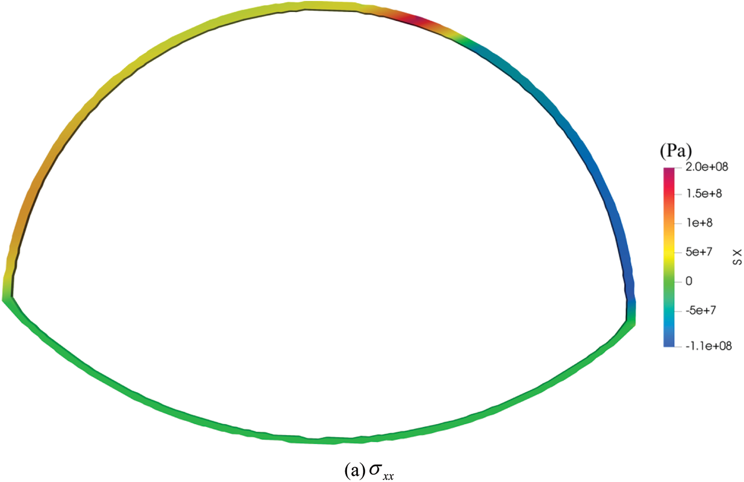
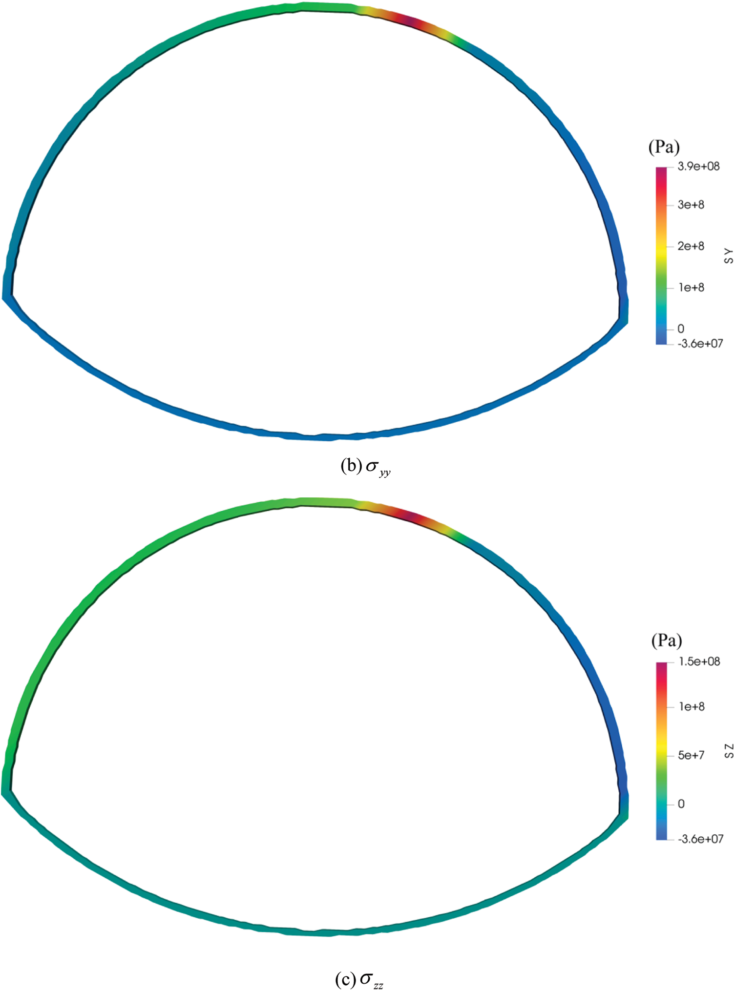
Figure 23: The normal stress field diagrams of lining with tunnel invert under bias pressure angle of 10 degree

5  Conclusion

The distribution location, expansion law, appearance, and generation mechanism of structural fractures in shallow tunnel lining under load are examined using PD, and the following main conclusions are drawn:

(1)   Through the comparative analysis with the laboratory test, it is concluded that the PD method is feasible in simulating the whole process of lining the initial crack, crack expansion, and overall failure.

(2)   The inner surface of the lining will create tensile cracks due to local bias pressure. It demonstrates that under the influence of bias pressure, the inner surface of the lining is primarily susceptible to tensile stress. Furthermore, the extended depth of the inner surface tensile crack is related to the bias pressure range.

(3)   When comparing and analyzing different lining thicknesses, the position of the crack in the loading process is roughly the same, but when the lining thickness is thin, the fracture propagation depth is larger, and new cracks will form around the primary crack. Therefore, the lining design should ensure that the lining has sufficient thickness.

(4)   Tensile stress is the main cause of lining failure, and the initial crack initiation occurs on the inner surface of the lining, not at the tip of the preset fracture, indicating that the inner surface of the lining is the location of the largest tensile stress. The preset tension crack is more harmful to the lining than the preset compression crack, and the preset crack at the arch waist of 30 degrees is more destructive to the lining than the preset crack of 60 degrees. The treatment of discovered tensile cracks should be prioritized in practical engineering.

Acknowledgement: The authors gratefully acknowledge the support from the National Natural Science Foundation of China (52079128).

Funding Statement: The paper is supported by the National Natural Science Foundation of China (52079128).

Conflicts of Interest: The authors declare that they have no conflicts of interest to report regarding the present study.

References

1. Xu, G., He, C., Chen, Z., Liu, C., Wang, B. et al. (2020). Mechanical behavior of secondary tunnel lining with longitudinal crack. Engineering Failure Analysis, 113(6), 104543. DOI 10.1016/j.engfailanal.2020.104543. [Google Scholar] [CrossRef]
2. Xu, G., He, C., Lu, D., Wang, S. (2019). The influence of longitudinal crack on mechanical behavior of shield tunnel lining in soft-hard composite strata. Thin-Walled Structures, 144(3), 106282. DOI 10.1016/j.tws.2019.106282. [Google Scholar] [CrossRef]
3. Liu, D., Li, M., Zuo, J., Gao, Y., Zhong, F. et al. (2021). Experimental and numerical investigation on cracking mechanism of tunnel lining under bias pressure. Thin-Walled Structures, 163, 107693. DOI 10.1016/j.tws.2021.107693. [Google Scholar] [CrossRef]
4. Lyu, Y., Wang, H., Gong, J. (2020). GPR detection of tunnel lining cavities and reverse-time migration imaging. Applied Geophysics, 17(1), 1–7. DOI 10.1007/s11770-019-0831-9. [Google Scholar] [CrossRef]
5. Zhao, D. P., Tan, X. R., Jia, L. L. (2014). Study on investigation and analysis of existing railway tunnel diseases. Applied Mechanics and Materials, 580–583, 1218–1222. DOI 10.4028/www.scientific.net/AMM.580-583.1218. [Google Scholar] [CrossRef]
6. Huang, S. P., Guo, M. L. (2015). Analysis and strategies of the common tunnel problems. Proceedings of the 2015 International Conference on Artificial Intelligence and Industrial Engineering, vol. 7, pp. 312–314. DOI 10.2991/aiie-15.2015.87. [Google Scholar] [CrossRef]
7. Goodman, R. E., Taylor, R. L., Brekke, T. L. (1968). A model for the mechanics of jointed rock. Journal of the Soil Mechanics and Foundations Division, 94(3), 637–659. DOI 10.1061/JSFEAQ.0001133. [Google Scholar] [CrossRef]
8. Desai, C. S., Zaman, M. M., Lightner, J. G., Siriwardane, H. J. (1984). Thin-layer element for interfaces and joints. International Journal for Numerical and Analytical Methods in Geomechanics, 8(1), 19–43. DOI 10.1002/(ISSN)1096-9853. [Google Scholar] [CrossRef]
9. Camacho, G. T., Ortiz, M. (1996). Computational modelling of impact damage in brittle materials. International Journal of Solids and Structures, 33(20), 2899–2938. DOI 10.1016/0020-7683(95)00255-3. [Google Scholar] [CrossRef]
10. Belytschko, T., Black, T. (1999). Elastic crack growth in finite elements with minimal remeshing. International Journal for Numerical Methods in Engineering, 45(5), 601–620. DOI 10.1002/(SICI)1097-0207(19990620)45:5<601::AID-NME598>3.0.CO;2-S. [Google Scholar] [CrossRef]
11. Moës, N., Dolbow, J., Belytschko, T. (1999). A finite element method for crack growth without remeshing. International Journal for Numerical Methods in Engineering, 46(1), 131–150. DOI 10.1002/(ISSN)1097-0207. [Google Scholar] [CrossRef]
12. Silling, S. A. (2000). Reformulation of elasticity theory for discontinuities and long-range forces. Journal of the Mechanics and Physics of Solids, 48(1), 175–209. DOI 10.1016/S0022-5096(99)00029-0. [Google Scholar] [CrossRef]
13. Silling, S. A., Bobaru, F. (2005). Peridynamic modeling of membranes and fibers. International Journal of Non-Linear Mechanics, 40(2), 395–409. DOI 10.1016/j.ijnonlinmec.2004.08.004. [Google Scholar] [CrossRef]
14. Silling, S. A., Askari, E. (2005). A meshfree method based on the peridynamic model of solid mechanics. Computers & Structures, 83(17), 1526–1535. DOI 10.1016/j.compstruc.2004.11.026. [Google Scholar] [CrossRef]
15. Zimmermann, M. (2005). A continuum theory with long-range forces for solids. USA: Massachusetts Institute of Technology. [Google Scholar]
16. Weckner, O., Emmrich, E. (2005). Numerical simulation of the dynamics of a non-local, inhomogeneous, infinite bar. Journal of Computational and Applied Mechanic, 6(2), 311–319. [Google Scholar]
17. Weckner, O., Abeyaratne, R. (2005). The effect of long-range forces on the dynamics of a bar. Journal of the Mechanics and Physics of Solids, 53(3), 705–728. DOI 10.1016/j.jmps.2004.08.006. [Google Scholar] [CrossRef]
18. Lehoucq, R. B., Silling, S. A. (2008). Force flux and the peridynamic stress tensor. Journal of the Mechanics and Physics of Solids, 56(4), 1566–1577. DOI 10.1016/j.jmps.2007.08.004. [Google Scholar] [CrossRef]
19. Foster, J. T., Silling, S. A., Chen, W. (2011). An energy based failure criterion for use with peridynamic states. International Journal for Multiscale Computational Engineering, 9(6), 675–688. DOI 10.1615/IntJMultCompEng.2011002407. [Google Scholar] [CrossRef]
20. Yu, H., Li, S. (2020). On energy release rates in peridynamics. Journal of the Mechanics and Physics of Solids, 142(3), 104024. DOI 10.1016/j.jmps.2020.104024. [Google Scholar] [CrossRef]
21. Shojaei, A., Mossaiby, F., Zaccariotto, M., Galvanetto, U. (2018). An adaptive multi-grid peridynamic method for dynamic fracture analysis. International Journal of Mechanical Sciences, 144(1), 600–617. DOI 10.1016/j.ijmecsci.2018.06.020. [Google Scholar] [CrossRef]
22. Huang, D., Lu, G., Liu, Y. (2015). Non-local peridynamic modeling and simulation on crack propagation in concrete structures. Mathematical Problems in Engineering, 2015(12), 1–11. DOI 10.1155/2015/571594. [Google Scholar] [CrossRef]
23. Yang, D., Dong, W., Liu, X., Yi, S., He, X. (2018). Investigation on mode-I crack propagation in concrete using bond-based peridynamics with a new damage model. Engineering Fracture Mechanics, 199(1), 567–581. DOI 10.1016/j.engfracmech.2018.06.019. [Google Scholar] [CrossRef]
24. Zhang, N., Gu, Q., Huang, S., Xue, X., Li, S. (2021). A practical bond-based peridynamic modeling of reinforced concrete structures. Engineering Structures, 244(1), 112748. DOI 10.1016/j.engstruct.2021.112748. [Google Scholar] [CrossRef]
25. Chen, Z., Chu, X. (2021). Peridynamic modeling and simulation of fracture process in fiber-reinforced concrete. Computer Modeling in Engineering & Sciences, 127(1), 241–272. DOI 10.32604/cmes.2021.015120. [Google Scholar] [CrossRef]
26. Zhou, X. P., Shou, Y. D. (2017). Numerical simulation of failure of rock-like material subjected to compressive loads using improved peridynamic method. International Journal of Geomechanics, 17(3), 4016086. DOI 10.1061/(ASCE)GM.1943-5622.0000778. [Google Scholar] [CrossRef]
27. Sun, B., Li, S., Gu, Q., Ou, J. (2019). Coupling of peridynamics and numerical substructure method for modeling structures with local discontinuities. Computer Modeling in Engineering & Sciences, 120(3), 739–757. DOI 10.32604/cmes.2019.05085. [Google Scholar] [CrossRef]
28. Underwood, P. (1983). Dynamic relaxation. Computer Methods in Applied Mechanics and Engineering, 1, 245–265. [Google Scholar]
29. Mashimo, H., Isago, N., Yoshinaga, S., Shiroma, H., Baba, K. (2002). Experimental investigation on load-carrying capacity of concrete tunnel lining. Japan Society of Civil Engineers, 2002, 1–11. [Google Scholar]
30. Mashimo, H., Kusaka, A., Isago, N., Kitani, T., Kaise, S. (2008). Experimental study on collapse mechanism of tunnel lining and effect of reinforcing material on load-bearing capacity of tunnel lining. Japan Society of Civil Engineers, 2008, 311–326. [Google Scholar]
31. Huang, H. W., Liu, D. J., Xue, Y. D., Wang, P. R., Liu, Y. (2013). Numerical analysis of cracking of tunnel linings based on extended finite element. Chinese Journal of Geotechnical Engineering, 35(2), 266–275. [Google Scholar]
32. Lei, M., Peng, L., Shi, C. (2015). Model test to investigate the failure mechanisms and lining stress characteristics of shallow buried tunnels under unsymmetrical loading. Tunnelling and Underground Space Technology, 46, 64–75. DOI 10.1016/j.tust.2014.11.003. [Google Scholar] [CrossRef]
33. He, B., Zhang, Z., Chen, Y. (2012). Unsymmetrical load effect of geologically inclined bedding strata on tunnels of passenger dedicated lines. Journal of Modern Transportation, 20(1), 24–30. DOI 10.1007/BF03325773. [Google Scholar] [CrossRef]
34. Liu, D., Li, M., Zuo, J., Gao, Y., Zhong, F. et al. (2021). Experimental and numerical investigation on cracking mechanism of tunnel lining under bias pressure. Thin-Walled Structures, 163, 107693. DOI 10.1016/j.tws.2021.107693. [Google Scholar] [CrossRef]
Cite This Article
Copyright © 2023 The Author(s). Published by Tech Science Press.
This work is licensed under a Creative Commons Attribution 4.0 International License , which permits unrestricted use, distribution, and reproduction in any medium, provided the original work is properly cited.
Downloads
Citation Tools