Dynamic Reliability Evaluation and Life Prediction of Transmission System of Multi-Performance Degraded Wind Turbine

Nomenclature

1  Introduction

With environmental pollution and energy shortages becoming more prominent, the development and utilization of new energy have become the focus of attention of all countries in the world. New energy will play a prominent role not only in improving the ecological environment and optimizing the energy structure, but also in promoting sustainable social and economic development. In addition to hydropower technology, wind power is the most mature, largest and most promising power generation method among new energy power generation technologies [1]. At present, many countries have invested a lot of research on wind power generation and related technologies.

Among various new energy, wind energy has the advantages of huge reserves, no pollution, no damage, no need for transportation and wide distribution [2–5]. For wind power generation, wind turbines are essential equipment. Their working status is closely related to the overall efficiency of wind power generation. And they are related to whether they can provide safe and reliable electricity for the lives of the general public [6].

The failures of large-scale wind turbines are mainly concentrated in the gear transmission system [7–9]. Wind farms are remote, while the rotating machinery of the generator set is bulky and high in the air. It is difficult to implement operations such as re-hoisting and component replacement [10]. Once a failure occurs, it is necessary to invest huge manpower and material resources in maintenance. With the development trend of higher and higher reliability requirements for mechanical products in various fields and smaller and smaller reliability test samples, the existing reliability evaluation methods have gradually failed to meet the engineering requirements on some occasions [11–17].

Under the influence of external random loads, multiple parameters of the wind turbine gear transmission system tend to change over time [18]. In addition, because the system operates in a harsh environment and is largely influenced by the internal gear-bearing, the failure modes of the major components exhibit some statistical correlation [19–21]. Therefore, when designing the wind turbine gear train, it is important to analyze the impact of failure correlation and time history on the system reliability. In reality, the load effect is usually regarded as a stochastic process. The corresponding functional functions can be constructed according to the relevant requirements, after which the dynamic reliability index of each component is analyzed by the perturbation method [22–24]. In addition, a simulation model is established for the transmission system. Then the reliability of the system is analyzed by simulation [25,26]. Since there are failure correlations among the system components, the simulation model corresponding to the strength degradation of the components can be constructed according to the requirements. Thereby, the laws of system stability and failure rate change with time can be analyzed.

The main research of this article is the dynamic reliability of planetary gear transmission systems. A stress-strength interference model based on performance degradation is introduced. Based on considering the strength degradation of each component, the improved Monte Carlo (MC) method simulation based on the Back Propagation (BP) neural network is used to obtain the curve of system reliability over time. Finally, using the Miner linear cumulative damage theory and the Carten-Dolan cumulative damage theory calculate the cumulative damage and fatigue life method of the gear transmission system.

2  Basic Theory of Reliability of Wind Turbine Gearbox

2.1 Basic Theory of Reliability

Reliability reflects the changing law of product quality on the time scale. It is the ability to complete the corresponding functions within the specified time according to different purposes, requirements and occasions [27,28]. Commonly used reliability characteristics include reliability, unreliability, average life and remaining life [29–31].

In the reliability calculation, interference analysis of random variables is required [32,33]. The basic idea is to compare the magnitude of the two random variables of stress and intensity. In the same coordinate system, the probability density function curves of stress and intensity usually intersect, which is called the “interference zone”. This shows that there is a possibility that the stress is greater than the strength. Use g(s) and f(s) to represent the probability density function of stress and strength, respectively. The reliability of the parts can be obtained by making the stress and strength interfere, as shown in Eq. (1).

R=∫0∞⁡g(s)[∫0∞⁡f(s)ds]ds(1)

Stress refers to various physical coefficients that may cause components to fail. And strength is a performance index for components to resist corresponding stress.

For engineering equipment, it is usually not an independent system, but is composed of multiple systems. This article mainly analyzes the wind power gear transmission system, which is a critical component of the wind power unit. Due to the complicated working conditions and the difficulty of maintenance, its reliability problems have largely hindered its further development.

Regarding the wind turbine transmission system, planetary gear transmission is generally adopted. In terms of planetary gear transmission, planetary carrier input is generally selected. The planetary gear is mainly used to effectively share the load. Fig. 1 [34] is a kind of gear transmission system in wind turbine. If helical gear transmission is selected, the corresponding overall structure is shown in Fig. 2.

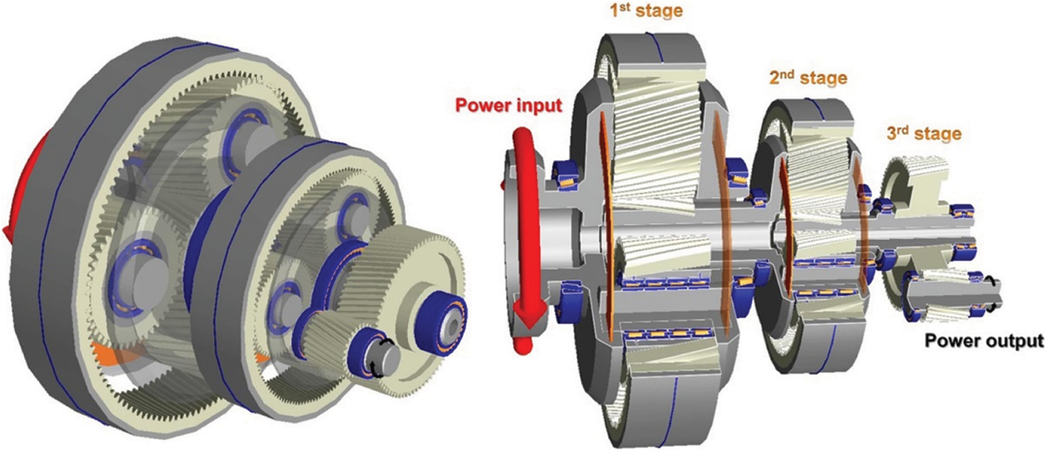
Figure 1: Gear transmission system in wind turbine

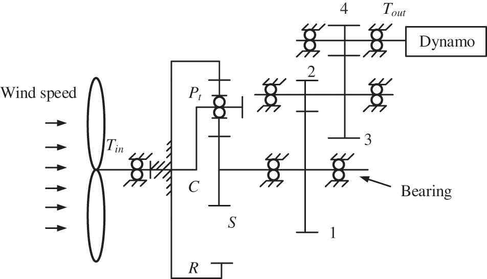
Figure 2: Wind turbine transmission system structure diagram
Note: Pi—Planetary gear; R—Internal gear; S—Sun gear; C—Planetary carrier; 1—Medium-speed driving helical gear; 2—Medium-speed driven helical gear; 3—High-speed driving helical gear; 4—High-speed driven helical gear; Tin—Input torque; Tout—Output torque.

Combining relevant experience results, it can be found that in the process of analyzing the reliability of the system, it focuses on the analysis of the impact of key components [35]. This article analyzes the reliability problems of the system composed of planetary carrier C and sun gear S. Generally speaking, the following assumptions can be made for tooth surface contact fatigue strength failure and tooth root bending fatigue strength [36–38]. During the operation of the gear, these two types of modes usually coexist and appear in multiple components of the gear. It can be determined that the strengths of the components in the two types of modes do not affect each other, but their loads show statistical correlation to a large extent. For tooth surface contact fatigue failure [39,40], only when the three-way component fails at the same time, the whole will have corresponding characteristics. For tooth root bending fatigue failure, if a planetary gear fails, the system will not work properly. Fig. 3 is the reliability diagram of the planetary gear transmission system.

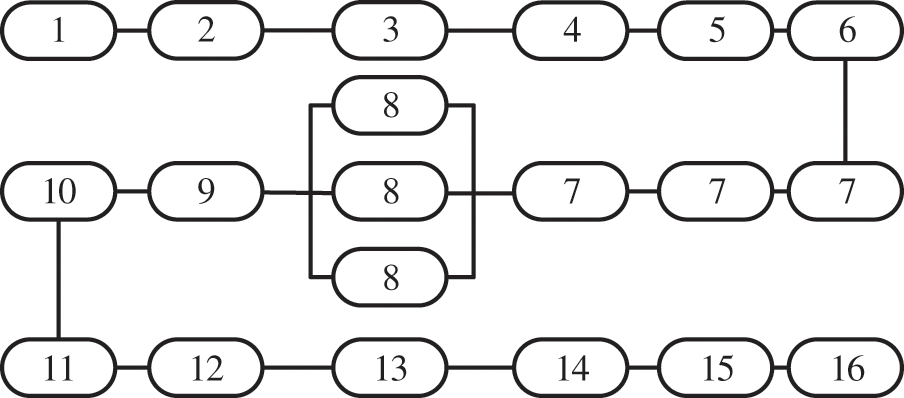
Figure 3: The reliability diagram of the plan

The specific meaning of the unit number is:

1, 3, 5——contact fatigue unit of each component;

2, 4, 6——bending fatigue unit of each component;

7, 8——bending fatigue unit and contact fatigue unit of planetary gear;

9, 11, 13, 15——contact fatigue units of helical gears 1, 2, 3 and 4;

10, 12, 14, 16——bending fatigue units of helical gear 1, 2, 3 and 4.

Combined with the above diagram, the following equation can be derived:

R=R1R2R3R4R5R6(R7)3[1−(1−R8)3]R9R10R11R12R13R14R15R16(2)

2.2 Failure Analysis of Gearbox of Wind Turbine

The wind turbine transmission system includes the main shaft, speed-increasing gearbox, high-speed output shaft, braking equipment, coupling and other components. The wind turbine captures wind energy through the wind wheel. The transmission system transfers the kinetic energy to the generator and converts it into electrical energy. The transmission system is located on top of the wind turbine tower. The height above the ground is generally tens of meters or even higher. Under the action of the alternating load with unstable wind, the transmission chain will shake as a whole.

The gearbox using the planetary gear transmission structure has many advantages such as smooth and precise meshing, power splitting and improvement of system load sharing. In addition, the safety coefficient of transmission system can be improved by reducing the size of the gearbox, reducing the weight, increasing the transmission efficiency, increasing the transmission ratio and increasing the load-bearing capacity. It is because the slight deformation of the planetary central axis makes the internal structure elastically adjusted. The load distribution of each planetary gear tends to be more consistent, so that the internal meshing is reasonably applied. Moreover, the planetary wheel and parallel wheel structure improve the ability of the system to resist impact loads and reduce the impact of components processing and assembly errors on the transmission.

This article mainly analyzes the main fault types of gearboxes and gears. Gearbox generally uses gear pairs to efficiently transmit power. The core function is variable speed. In addition, the types of gearboxes mainly involve cylindrical gearboxes, combined gearboxes, etc. Relevant statistics show that gearbox failures account for 40%–50% of the total failures, which is a relatively high proportion in wind turbines. The assembly space is not large for a gearbox, but it must bear the impact load of changing directions and changing loads. In addition, due to its complex failure causes, maintenance is more difficult. Therefore, it needs to be studied, which is significant to the avoidance of fault problems.

3  Dynamic Reliability Modeling of Gear Transmission System Considering Strength Degradation

Under the influence of external random loads, many parameters of the wind turbine gear transmission system tend to change over time [41]. In addition, the operating environment of the system is relatively harsh and is largely affected by the internal gear-bearings, the failure modes of the main components show a certain correlation. Thus, when designing a wind turbine gear transmission system, it is necessary to analyze the influence of failure correlation and time history on system reliability. In reality, the load effect is usually regarded as a random process. While the function can be constructed according to relevant requirements. Then analyze the dynamic reliability index of each component by the perturbation method. Because of the existence of the failure correlation between the components of the system, the simulation model corresponding to the strength degradation of the components can be constructed according to the requirements. Then the law of system reliability changing with time can be analyzed.

3.1 Reliability Calculation Model

The strength and stress change over time. When the strength of the product degrades over time, the interference area of the strength and stress will become larger over time. It reflects that the reliability of the product is gradually decreasing. Therefore, the strength X that the product can bear and the stress Y applied by the external are both variables that change over time. The strength X of the product and the stress Y imposed by the external are regarded as random processes X(t) and Y(t). In contrast, symmetric and homogeneous drift Brownian motion is used to describe the random variables.

X(t)=σB1B(t)+d(s)⋅t+μ1(3)

Y(t)=σB2B(t)+μ2(4)

where B(t)——Standard Brownian motion with mean value 0 and variance t; σB——Diffusion coefficient, usually constant; d(s)——Drift coefficient; μ——Starting point of drift Brownian motion, where μ1 refers to the initial strength of the product, and μ2 refers to the initial value of the stress. The density function can be obtained through Z(t)=X(t)−Y(t):

ht(z,t)=12πσB2texp⁡[−z−(d(s)⋅t−μz)22tσB2](5)

Product reliability is R=P(Z(t)>0)=P(X(t)−Y(t)>0). The intensity degradation is a negative drift Brownian motion, that is d(s)<0. Combined with the distribution of the first arrival time of Brownian motion, the working reliability in time (0,t0) is:

Rt0=P(Z(t)>0)=∫t0∞|μz|2πt3σB2exp⁡[−(d(s)t+μz)22tσB2]dz(6)

According to Eq. (6) and numerical integration calculation, when the time tends to 0, the product reliability is 1.

When using the time-related stress intensity interference model to solve the reliability of the product after working t hours, the product reliability can be expressed:

R=P(Z>0)⋅P(X(t)−Y(t)>0)=Rt0⋅Rz(7)

When t=0,R=Rz.

3.2 Time-Varying Stress Calculation Model

Tooth surface contact stress can be calculated as follows [42]:

σH=ZEZHZεZβKAKVKHβKHαFtd1b⋅μ±1μ(8)

where ZE is the elastic coefficient; ZH is the node area coefficient; Zε is the coincidence degree function; Zβ is the helix angle coefficient; KA is the use coefficient; KV is the tooth load distribution coefficient; KHα is the tooth load distribution coefficient calculated for the contact strength; KHβ is the tooth between teeth load distribution coefficient; Ft is the circumferential force; d1 is the diameter of the dividing circle; b is the medium and small tooth width; μ is the gear ratio, μ=z2z1=d2d1; z2, z1 are the number of teeth corresponding to the two types of gears.

The limit of tooth surface contact fatigue stress can be analyzed by the following equation:

σHS=σHlimZNZRZVZWZLZX(9)

where σHlim denotes the contact fatigue limit of the experimental gear; ZN denotes the life coefficient; ZR denotes the roughness coefficient; ZV denotes the speed coefficient; ZL denotes the lubricant coefficient; ZW denotes the work hardening coefficient; ZX denotes the size coefficient.

Based on the analysis of relevant specifications, the mean value and coefficient of variation can be deduced as follows [42]:

σHS¯=σ¯HlimZ¯NZ¯LZ¯VZ¯RZ¯WZ¯X(10)

CσHS=(CσHlim2+CZN2+CZL2+CZV2+CZR2+CZW2+CZX2)12(11)

The mean value and coefficient of variation of σHlim can be analyzed by the following equations:

σ¯Hlim=exp⁡(2.326Sln⁡σHlim+ln⁡σHlim+12S2ln⁡σHlim)(12)

CσHlim=eSln⁡σHlim2−1(13)

where Sln⁡σHlim mainly refers to the logarithmic standard deviation, which can be found in the manual [43].

The tooth root bending fatigue stress can be calculated as follows:

σF=KAKVKFβKFαFtbmnYFαYSαYεYβ(14)

where YFα denotes the tooth profile coefficient; YSα denotes the stress correction coefficient; Yε denotes the coincidence coefficient; Yβ denotes the helix angle coefficient; Ft denotes the circumferential force; KA denotes the use coefficient; KV denotes the dynamic load coefficient; KFβ denotes the tooth load distribution coefficient; KFα denotes the load distribution coefficient between teeth; mn denotes the normal modulus; b denotes the smaller tooth width.

The limit of bending fatigue stress can be analyzed by the following equation:

σFS=σFlimYSTYNTYδRrelTYRrelTYX(15)

where σFlim denotes the tooth root bending fatigue limit stress; YST denotes the stress correction coefficient; YNT denotes the life coefficient; YδrelT denotes the sensitivity coefficient; YRrelT denotes the condition system; YX denotes the specification coefficient.

In addition, the mean value and coefficient of variation of this parameter can be calculated as follows [43]:

σFS¯=σ¯FlimY¯NTY¯STY¯δrelTY¯RrelTY¯X(16)

CσHS=(CσHlim2+CZN2+CZL2+CZV2+CZR2+CZW2+CZX2)12(17)

The mean value of σFlim can be analyzed by the following equations:

δ¯Flim=exp⁡(2.326Sln⁡σFlim+ln⁡σFlim+12Sln⁡σFlim2)(18)

CσFlim=eSln⁡σFlim2−1(19)

where Sln⁡σFlimis the logarithmic standard deviation, which can be found in the manual [43].

3.3 Dynamic Reliability Model Considering Strength Degradation

Because the strength is gradually degraded under the action of long-term load, the dynamic reliability model of the component of the stress-strength interference model is:

R(t)=P(r(t)>S(t))(20)

R(t)=P(r(t)>S(t))R0(21)

where t=0,R(t)=R0.

After the MC method is used to carry out the simulation analysis, the K-S test can be carried out according to the requirements. Then it can be concluded that its strength obeys the normal distribution law. At the same time, the parameters corresponding to all components conform to the Weibull distribution characteristics as a whole. At this time, they can be converted to a normal distribution. In this section, an MC improvement based on the BP neural network (BP-MC) is used [44]. The purpose is to input the sample points into the BP model when identifying whether the MC sample points are located in the failure domain. This is to shorten the calculation time required for the sample points, thereby improving the calculation efficiency. When selecting the training set, a DOE experiment is performed to select sample points in the entire design space. The performance function value of the sample points is used as the screening criterion. The sample points close to the failure surface are also added to the training set. Put the sample points of the training set into the reliability function model. The function value of its equation is further calculated as a response set. The BP model can be trained by taking the training set as the input and the response set as the output. When using the BP model, the predicted value of the sample point input into the BP model is not important; only the positive and negative values need to be paid attention to. On the failure surface, the function value of the limit state equation is 0; in the safety domain, the function value of the limit state equation is positive; and in the failure domain, the function value of the limit state equation is negative. As long as the accuracy of the BP model near the failure surface is guaranteed, both the failure domain and the safety domain are covered by the DOE. The BP model can be used to identify whether the MC sample points are located in the failure domain, thereby completing the reliability calculation of the structure. The specific process of the method is shown in Fig. 4.

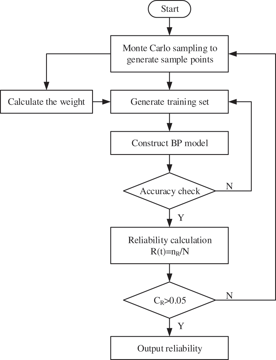
Figure 4: Steps of BP-MC method for calculating reliability

First, determine the equivalent stress Y(t) and strength X(t) distribution of the component under time-varying load. Then calculate the initial reliability [45]. The total number of samples sampled by MC method is N, the design variables contained in each point are counted as Wij(j=1,2,…,n), where n is the number of design variables. The probability of the sample point appearing in the design space is used as the weight. This section involves two variables, stress Y(t) and strength X(t), which are independent of each other. The weight is expressed as Eq. (22):

wi=fi(Ui1)fi(Ui2)…fn(Uin)=fi(Xi(t))fi(Yi(t))(22)

where fn(⋅) is the probability density function of the n-th random variable. Select sample points in the design space as the BP training set. Then sort the remaining samples by weight, select the part of the sample points with the lowest weight to join the BP training set, while substitute the sample points into the function Z(Xi(t),Yi(t)). Then use the training set [Xi(t),Yi(t)] as input and the response set Z(Xi(t),Yi(t)) as the output to obtain the initial BP model. Use Matlab to predict the response value of the spatial sample points Z~(Xi(t)Yi(t)). Arrange the obtained predicted values Z~(Xi(t)Yi(t)) according to the absolute value. Then compare the error with the true value. If it does not meet the accuracy requirements of the BP model, return and retrain; if it does, use the response prediction value for reliability calculation. Put the sample value into the BP model and get the value of Z~(Xi(t)Yi(t)), when Z~(Xi(t)Yi(t))>0, the system is reliable, the total number of reliable points is L, then the system reliability is:

R(t)=L/N(23)

Use the MC method to calculate, only when N is large enough, the obtained result is reliable. Therefore, the obtained result needs to be checked. This section uses the standard deviation to determine. Suppose CR=1−R(t)R(t)N, when there are enough samples, the set condition can be satisfied: CR is less than 0.05.

If CR is less than 0.05, the reliability is output. If not, return to the first step, add more samples. Then construct the BP model of the new sample point. Repeat the above steps until the judgment conditions are met. Finally, output the reliability.

Take the 1.5 MW wind turbine transmission system as an example.

The radius of the impeller is 26.8 m. Input shaft speed is 14.6 r/min, rated impeller torque is 1.25 × 106 Nm, rated wind speed is 12 m/s, wind energy coefficient is 0.55, gear material is 20CrMnTi, cut-in wind speed is 4 m/s, cut-out wind speed is 20 m/s, sun gear tooth number is 27, planetary gear tooth number is 44, internal gear tooth number is 115, gear 1 tooth number is 103, gear 2 teeth number is 24, gear 3 teeth number is 99, gear 7 teeth number is 24, low-speed shaft modulus is 16, meshing angle is 23°; medium-speed shaft normal surface modulus is 12, helix angle is 10.5°, meshing angle is 21°; high-speed shaft normal surface modulus is 24, helix angle is 12.5, meshing angle is 21°, random wind speed is v∼W (k = 4.5065, c = 13.1485). Each parameter is considered to obey a normal distribution, while its mean and variance are from references [46,47].

Under time-varying load conditions, during the analysis of gears’ reliability, the focus is on the problems caused by pitting on the tooth surface. Refer to Figs. 5a–5h for details of the changes in the reliability of each gear over time.

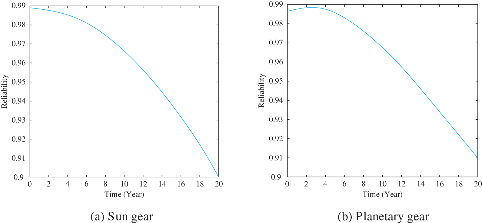
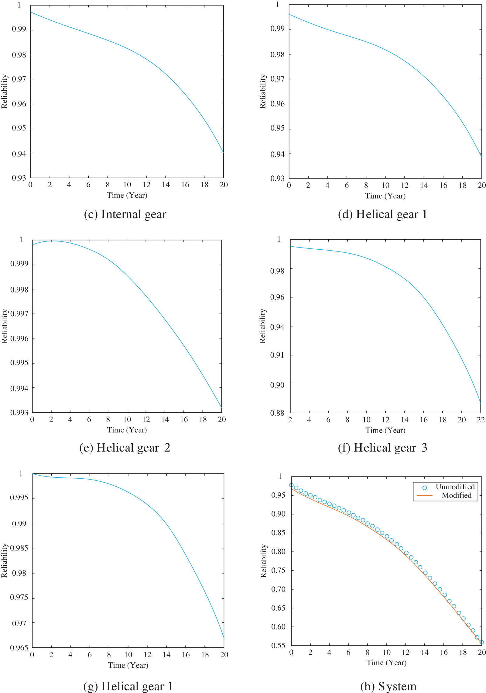
Figure 5: Changes in the reliability of each gear element over time

Combining Figs. 5a–5h, it can be found that the reliability of all gears has shown a continuous decrease with the extension of time. The reliability curve obtained by the modified stress-strength reliability model will move down compared to the unmodified reliability model, so that the modified reliability model is more reliable.

4  Prediction and Analysis of Fatigue Life of Wind Power Gear Transmission System

4.1 Nominal Stress Method

For all structures, if there is no difference in the stress concentration coefficient and the load spectrum, their life will be the same. This method generally uses load statistical analysis to clarify the nominal stresses corresponding to all stressed parts. Then estimates the fatigue life in combination with related theories [48,49]. In addition, the nominal stress method can not only analyze the service life of a component under a specific stress amplitude through the S-N or P-S-N curve, but also can be combined with the cumulative damage theory to achieve scientific fatigue design. Among P-S-N, S represents stress, N represents cycles, and P represents survival rate.

Usually, due to the lack of components of the same shape, the P-S-N curve is modified under uniaxial loading of similar materials to calculate the fatigue life of the component [50,51]. The process for estimating the fatigue life of the structure is as follows:

(1)   Clarify the stress dangerous parts;

(2)   Define the nominal stress in conjunction with related manuals to determine the stress concentration coefficient KT;

(3)   Query the P-S-N curve of the material. If there is a lack, it can be replaced by the P-S-N curve of similar materials;

(4)   Combining the fatigue damage accumulation theory, calculate the fatigue life of components.

4.2 Load Statistics

The gear transmission system operates in a diverse environment. Because the gear transmission system is affected by random loads, the components tend to form alternating stresses, which leads to the accumulation of internal damage and fatigue failure of the components. In the fatigue reliability analysis of components, the statistical analysis of stress-time history uses the rain flow counting method [52]. Then obtain the stress spectrum and probability distribution function of a load of each component of the transmission system, to analyze the load action history of the wind turbine in the working process. The stress-strength interference model is applied to the reliability analysis and life prediction of the transmission system.

The stress spectrum of each component is shown in Figs. 6a–6e:

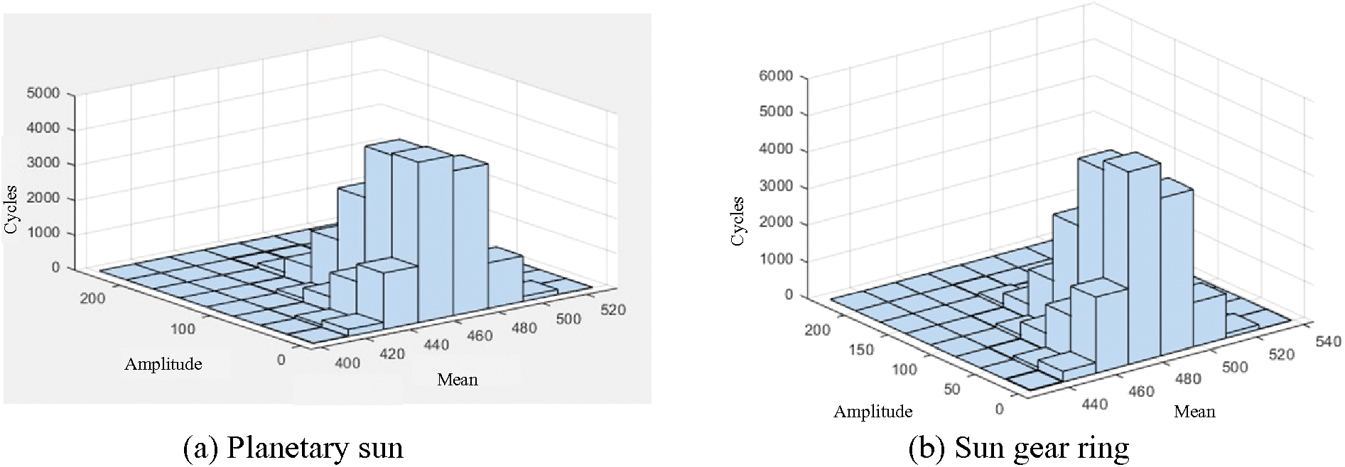
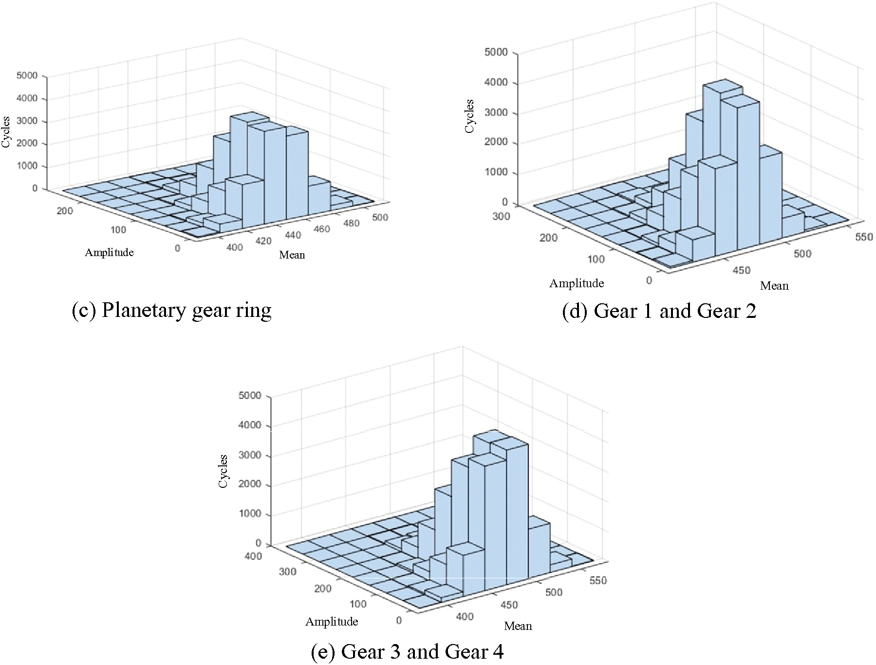
Figure 6: The stress spectrum of each component

4.3 Fatigue Life Estimation of Transmission System

Because the random wind speed is constantly changing, the stress applied to each component also changes non-directionally. To clarify the fatigue life, not only can the P-S-N curve be used, but also the fatigue cumulative damage criterion can be used to carry out the analysis. The dynamic random stress of each gear pair of the transmission system is counted cyclically. Then the P-S-N curve of the transmission system component is obtained according to the fatigue performance of the material. Finally, use the Miner linear cumulative damage theory and Corten-Dolan cumulative damage theory to calculate the cumulative damage and fatigue life of the gears of the wind turbine gear transmission system under random wind loads. It is a reliable and effective fatigue life prediction method.

The gear material is 20GrMnTi, while the bearing material is high-strength bearing steel GCr15SiMnA. Assume that the wind turbine gear transmission system works 20 h a day. Combined with the rain flow calculation program, the number of cycles corresponding to the stress amplitude at each level should be clarified. At this time, the contact stress spectrum should be equivalent to the contact stress through the Goodman equation. Then the fatigue life equation will be used as the core. The total working time when the gear in the transmission system is damaged can be calculated as shown in Table 1.

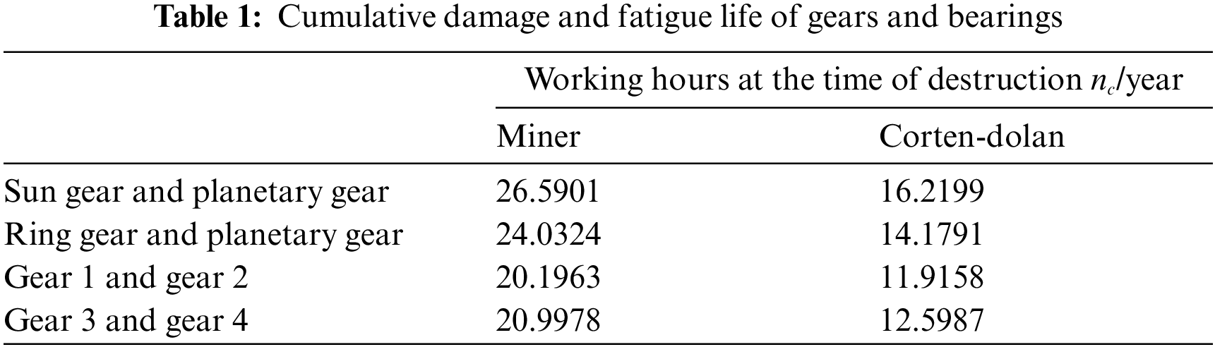
It can be found that with the continuous increase of input torque, the gear stress has further increased. The limit value of the contact stress is about 1000 MPa. However, it can be found in combination with the fatigue damage theory that because the speed of the planetary gear is relatively low, the corresponding contact damage of the high-speed gear is relatively large, and its useful life is relatively short. In addition, the fatigue life calculated by Carten-Dolan theory of each component is smaller than that of Miner theory, indicating that Carten-Dolan damage theory is more reliable than Miner theory.

5  Conclusion

This article mainly analyzes and evaluates the dynamic reliability of the planetary gear transmission system. Based on the strength degradation of each component, a stress-strength interference model based on performance degradation is introduced. Through the BP-MC, the system reliability curve with time is obtained. Finally, Miner linear cumulative damage theory and Carten-Dolan cumulative damage theory are used to calculate the cumulative damage and fatigue life of gears in the transmission system. The results show that Carten-Dolan damage theory is more reliable than Miner theory.

Acknowledgement: The supports from the National Natural Science Foundation of China (Grant Nos. 52075081 and 52175130), the Innovation Training Programme for Chengdu university Students (CDUCX2022047), and The Key Laboratory of Pattern Recognition and Intelligent Information Processing, Institutions of Higher Education of Sichuan Province, Chengdu University, China (MSSB-2022-08) are gratefully acknowledged.

Funding Statement: The authors received no specific funding for this study.

Conflicts of Interest: The authors declare that they have no conflicts of interest to report regarding the present study.

References

1. Porté-Agel, F., Bastankhah, M., Shamsoddin, S. (2020). Wind-turbine and wind-farm flows: A review. Boundary-Layer Meteorology, 174(1), 1–59. DOI 10.1007/s10546-019-00473-0. [Google Scholar] [CrossRef]
2. Shoaib, M., Siddiqui, I., Rehman, S., Khan, S., Alhems, L. M. (2019). Assessment of wind energy potential using wind energy conversion system. Journal of Cleaner Production, 216, 346–360. DOI 10.1016/j.jclepro.2019.01.128. [Google Scholar] [CrossRef]
3. Liu, H., Chen, C., Lv, X., Wu, X., Liu, M. (2019). Deterministic wind energy forecasting: A review of intelligent predictors and auxiliary methods. Energy Conversion and Management, 195, 328–345. DOI 10.1016/j.enconman.2019.05.020. [Google Scholar] [CrossRef]
4. Li, X. Q., Song, L. K., Bai, G. C. (2022). Recent advances in reliability analysis of aeroengine rotor system: A review. International Journal of Structural Integrity, 13(1), 1–29. DOI 10.1108/IJSI-10-2021-0111. [Google Scholar] [CrossRef]
5. Meng, D., Li, Y., He, C., Guo, J., Lv, Z. et al. (2021). Multidisciplinary design for structural integrity using a collaborative optimization method based on adaptive surrogate modelling. Materials & Design, 206, 109789. DOI 10.1016/j.matdes.2021.109789. [Google Scholar] [CrossRef]
6. Bortolotti, P., Ivanov, H., Johnson, N., Barter, G. E., Veers, P. et al. (2022). Challenges, opportunities, and a research roadmap for downwind wind turbines. Wind Energy, 25(2), 354–367. DOI 10.1002/we.2676. [Google Scholar] [CrossRef]
7. Meng, D., Wang, H., Yang, S., Lv, Z., Hu, Z. et al. (2022). Fault analysis of wind power rolling bearing based on EMD feature extraction. Computer Modeling in Engineering & Sciences, 130(1), 543–558. DOI 10.32604/cmes.2022.018123. [Google Scholar] [CrossRef]
8. He, P., Hong, R., Wang, H., Lu, C. (2018). Fatigue life analysis of slewing bearings in wind turbines. International Journal of Fatigue, 111, 233–242. DOI 10.1016/j.ijfatigue.2018.02.024. [Google Scholar] [CrossRef]
9. Menezes, E. J. N., Araújo, A. M., da Silva, N. S. B. (2018). A review on wind turbine control and its associated methods. Journal of Cleaner Production, 174, 945–953. DOI 10.1016/j.jclepro.2017.10.297. [Google Scholar] [CrossRef]
10. de Novaes Pires Leite, G., Araújo, A. M., Rosas, P. A. C. (2018). Prognostic techniques applied to maintenance of wind turbines: A concise and specific review. Renewable and Sustainable Energy Reviews, 81, 1917–1925. DOI 10.1016/j.rser.2017.06.002. [Google Scholar] [CrossRef]
11. Meng, D., Yang, S., Zhang, Y., Zhu, S. P. (2019). Structural reliability analysis and uncertainties-based collaborative design and optimization of turbine blades using surrogate model. Fatigue & Fracture of Engineering Materials & Structures, 42(6), 1219–1227. DOI 10.1111/ffe.12906. [Google Scholar] [CrossRef]
12. Bangalore, P., Letzgus, S., Karlsson, D., Patriksson, M. (2017). An artificial neural network-based condition monitoring method for wind turbines, with application to the monitoring of the gearbox. Wind Energy, 20(8), 1421–1438. DOI 10.1002/we.2102. [Google Scholar] [CrossRef]
13. Zhu, S. P., Keshtegar, B., Tian, K., Trung, N. T. (2021). Optimization of load-carrying hierarchical stiffened shells: Comparative survey and applications of six hybrid heuristic models. Archives of Computational Methods in Engineering, 28(5), 4153–4166. DOI 10.1007/s11831-021-09528-3. [Google Scholar] [CrossRef]
14. Nahal, M., Khelif, R. (2020). A finite element model for estimating time-dependent reliability of a corroded pipeline elbow. International Journal of Structural Integrity, 12(2), 306–321. DOI 10.1108/IJSI-02-2020-0021. [Google Scholar] [CrossRef]
15. Liu, X., Wang, X., Xie, J., Li, B. (2020). Construction of probability box model based on maximum entropy principle and corresponding hybrid reliability analysis approach. Structural and Multidisciplinary Optimization, 61(2), 599–617. DOI 10.1007/s00158-019-02382-9. [Google Scholar] [CrossRef]
16. Liu, X., Liang, R., Hu, Y., Tang, X., Bastien, C. et al. (2021). Collaborative optimization of vehicle crashworthiness under frontal impacts based on displacement oriented structure. International Journal of Automotive Technology, 22(5), 1319–1335. DOI 10.1007/s12239-021-0115-2. [Google Scholar] [CrossRef]
17. Liu, X., Gong, M., Zhou, Z., Xie, J., Wu, W. (2021). An improved first order approximate reliability analysis method for uncertain structures based on evidence theory. Mechanics Based Design of Structures and Machines, 1–18. DOI 10.1080/15397734.2021.1956324. [Google Scholar] [CrossRef]
18. Cui, D., Wang, G., Lu, Y., Sun, K. (2020). Reliability design and optimization of the planetary gear by a GA based on the DEM and Kriging model. Reliability Engineering & System Safety, 203, 107074. DOI 10.1016/j.ress.2020.107074. [Google Scholar] [CrossRef]
19. Yuan, R., Tang, M., Wang, H., Li, H. (2019). A reliability analysis method of accelerated performance degradation based on Bayesian strategy. IEEE Access, 7, 169047–169054. DOI 10.1109/Access.6287639. [Google Scholar] [CrossRef]
20. Yuan, R., Li, H., Gong, Z., Tang, M., Li, W. (2017). An enhanced Monte Carlo simulation–based design and optimization method and its application in the speed reducer design. Advances in Mechanical Engineering, 9(9). DOI 10.1177/1687814017728648. [Google Scholar] [CrossRef]
21. Abd Rahim, A. A., Abdullah, S., Singh, S. S. K., Nuawi, M. Z. (2019). Reliability assessment on automobile suspension system using wavelet analysis. International Journal of Structural Integrity, 10(5), 602–611. DOI 10.1108/IJSI-04-2019-0035. [Google Scholar] [CrossRef]
22. Li, H., Yuan, R., Fu, J. (2019). A reliability modeling for multi-component systems considering random shocks and multi-state degradation. IEEE Access, 7, 168805–168814. DOI 10.1109/Access.6287639. [Google Scholar] [CrossRef]
23. Zhi, P., Xu, Y., Chen, B. (2019). Time-dependent reliability analysis of the motor hanger for EMU based on stochastic process. International Journal of Structural Integrity, 11(3), 453–469. DOI 10.1108/IJSI-07-2019-0075. [Google Scholar] [CrossRef]
24. Pavlou, D. G. (2018). The theory of the SN fatigue damage envelope: Generalization of linear, double-linear, and non-linear fatigue damage models. International Journal of Fatigue, 110, 204–214. DOI 10.1016/j.ijfatigue.2018.01.023. [Google Scholar] [CrossRef]
25. Babich, D., Bastun, V., Dorodnykh, T. (2019). Structural-probabilistic modeling of fatigue failure under elastic-plastic deformation. International Journal of Structural Integrity, 10(4), 484–496. DOI 10.1108/IJSI-05-2018-0024. [Google Scholar] [CrossRef]
26. Zhu, S. P., Ai, Y., Liao, D., Correia, J. A., De Jesus, A. M. et al. (2021). Recent advances on size effect in metal fatigue under defects: A review. International Journal of Fracture, 234, 21–43. DOI 10.1007/s10704-021-00526-x. [Google Scholar] [CrossRef]
27. Yang, Y. J., Wang, G., Zhong, Q., Zhang, H., He, J. et al. (2021). Reliability analysis of gas pipeline with corrosion defect based on finite element method. International Journal of Structural Integrity, 12(6), 854–863. DOI 10.1108/IJSI-11-2020-0112. [Google Scholar] [CrossRef]
28. Zhu, S. P., Keshtegar, B., Trung, N. T., Yaseen, Z. M., Bui, D. T. (2019). Reliability-based structural design optimization: Hybridized conjugate mean value approach. Engineering with Computers, 37(1), 381–394. DOI 10.1007/s00366-019-00829-7. [Google Scholar] [CrossRef]
29. Meng, D., Yang, S., Lin, T., Wang, J., Yang, H. et al. (2022). RBMDO using Gaussian mixture model-based second-order mean-value saddlepoint approximation. Computer Modeling in Engineering & Sciences, 132(2), 553–568. DOI 10.32604/cmes.2022.020756. [Google Scholar] [CrossRef]
30. Meng, D., Hu, Z., Guo, J., Lv, Z., Xie, T. et al. (2021). An uncertainty-based structural design and optimization method with interval taylor expansion. Structures, 33, 4492–4500. DOI 10.1016/j.istruc.2021.07.007. [Google Scholar] [CrossRef]
31. Meng, D., Yang, S., He, C., Wang, H., Lv, Z. et al. (2022). Multidisciplinary design optimization of engineering systems under uncertainty: A review. International Journal of Structural Integrity, 13(4), 565–593. DOI 10.1108/IJSI-05-2022-0076. [Google Scholar] [CrossRef]
32. Meng, D., Xie, T., Wu, P., He, X., Hu, Z. et al. (2021). An uncertainty-based design optimization strategy with random and interval variables for multidisciplinary engineering systems. Structures, 32, 997–1004. DOI 10.1016/j.istruc.2021.03.020. [Google Scholar] [CrossRef]
33. Blokus-Roszkowska, A., Kołowrocki, K. (2017). Modelling safety of multistate systems with dependent components and subsystems. Journal of Polish Safety and Reliability Association, 8(3), 23–42. [Google Scholar]
34. Yan, Y. (2020). Load characteristic analysis and fatigue reliability prediction of wind turbine gear transmission system. International Journal of Fatigue, 130, 105259. [Google Scholar]
35. Zhu, S. P., Keshtegar, B., Bagheri, M., Hao, P., Trung, N. T. (2020). Novel hybrid robust method for uncertain reliability analysis using finite conjugate map. Computer Methods in Applied Mechanics and Engineering, 371, 113309. DOI 10.1016/j.cma.2020.113309. [Google Scholar] [CrossRef]
36. Yuan, R., Li, H., Wang, Q. (2019). Simulation-based design and optimization and fatigue characteristics for high-speed backplane connector. Advances in Mechanical Engineering, 11(6). DOI 10.1177/1687814019856752. [Google Scholar] [CrossRef]
37. Narayanan, G. (2020). Probabilistic fatigue model for cast alloys of aero engine applications. International Journal of Structural Integrity, 12(3), 454–469. DOI 10.1108/IJSI-05-2020-0048. [Google Scholar] [CrossRef]
38. He, J. C., Zhu, S. P., Liao, D., Niu, X. P. (2020). Probabilistic fatigue assessment of notched components under size effect using critical distance theory. Engineering Fracture Mechanics, 235, 107150. DOI 10.1016/j.engfracmech.2020.107150. [Google Scholar] [CrossRef]
39. Liu, X., Zhang, Y., Xie, S., Zhang, Q., Guo, H. (2019). Fatigue failure analysis of express freight sliding side covered wagon based on the rigid-flexibility model. International Journal of Structural Integrity, 12(1), 98–108. DOI 10.1108/IJSI-11-2019-0122. [Google Scholar] [CrossRef]
40. Salari, M. (2019). Fatigue crack growth reliability analysis under random loading. International Journal of Structural Integrity, 11(2), 157–168. DOI 10.1108/IJSI-06-2019-0053. [Google Scholar] [CrossRef]
41. Li, W., Gao, L., Garg, A., Xiao, M. (2020). Multidisciplinary robust design optimization considering parameter and metamodeling uncertainties. Engineering with Computers, 38, 191–208. DOI 10.1007/s00366-020-01046-3. [Google Scholar] [CrossRef]
42. Meng, D., Lv, Z., Yang, S., Wang, H., Xie, T. et al. (2021). A time-varying mechanical structure reliability analysis method based on performance degradation. Structures, 34, 3247–3256. DOI 10.1016/j.istruc.2021.09.085. [Google Scholar] [CrossRef]
43. Lynwander, P. (2019). Gear drive systems: Design and application. USA: CRC Press. [Google Scholar]
44. Heravi, A. R., Hodtani, G. A. (2018). A new correntropy-based conjugate gradient backpropagation algorithm for improving training in neural networks. IEEE Transactions on Neural Networks and Learning Systems, 29(12), 6252–6263. DOI 10.1109/TNNLS.2018.2827778. [Google Scholar] [CrossRef]
45. Xu, H., Li, W., Li, M., Hu, C., Zhang, S. et al. (2018). Multidisciplinary robust design optimization based on time-varying sensitivity analysis. Journal of Mechanical Science and Technology, 32(3), 1195–1207. DOI 10.1007/s12206-018-0223-8. [Google Scholar] [CrossRef]
46. Carter, A. D. (2016). Mechanical reliability. UK: Macmillan International Higher Education. [Google Scholar]
47. Woo, S. (2020). Reliability design of mechanical systems. Singapore: Springer. [Google Scholar]
48. Liao, D., Zhu, S. P., Keshtegar, B., Qian, G., Wang, Q. (2020). Probabilistic framework for fatigue life assessment of notched components under size effects. International Journal of Mechanical Sciences, 181, 105685. DOI 10.1016/j.ijmecsci.2020.105685. [Google Scholar] [CrossRef]
49. Abdullah, L., Singh, S. S. K., Azman, A. H., Abdullah, S., Ihsan, A. K. A. M. et al. (2019). Fatigue life-based reliability assessment of a heavy vehicle leaf spring. International Journal of Structural Integrity, 10(5), 726–736. DOI 10.1108/IJSI-04-2019-0034. [Google Scholar] [CrossRef]
50. Nya, R. M., Abdullah, S., Singh, S. S. K. (2019). Reliability-based fatigue life of vehicle spring under random loading. International Journal of Structural Integrity, 10(5), 737–748. DOI 10.1108/IJSI-03-2019-0025. [Google Scholar] [CrossRef]
51. Li, S., Liu, X., Wang, X., Wang, Y. (2019). Fatigue life prediction for automobile stabilizer bar. International Journal of Structural Integrity, 11(2), 303–323. DOI 10.1108/IJSI-07-2019-0063. [Google Scholar] [CrossRef]
52. Kebir, T., Correia, J., Benguediab, M., de Jesus, A. M. (2020). Numerical study of fatigue damage under random loading using rainflow cycle counting. International Journal of Structural Integrity, 12(1), 149–162. DOI 10.1108/IJSI-04-2020-0041. [Google Scholar] [CrossRef]
Cite This Article
Copyright © 2023 The Author(s). Published by Tech Science Press.
This work is licensed under a Creative Commons Attribution 4.0 International License , which permits unrestricted use, distribution, and reproduction in any medium, provided the original work is properly cited.
Downloads
Citation Tools