
 Submit a Paper
 Propose a Special lssue
 Open Access
ARTICLE

Study of Fractional Order Dynamical System of Viral Infection Disease under Piecewise Derivative
1 Department of Mathematics and Sciences, Prince Sultan University, P.O. Box 66833, Riyadh, 11586, Saudi Arabia
2 Department of Mathematics, University of Malakand, Chakdara Dir(L), Khyber Pakhtunkhwa, 18000, Pakistan
3 Department of Medical Research, China Medical University, Taichung, 40402, Taiwan
* Corresponding Author: Thabet Abdeljawad. Email:
(This article belongs to the Special Issue: Applications of Fractional Operators in Modeling Real-world Problems: Theory, Computation, and Applications)
Computer Modeling in Engineering & Sciences 2023, 136(1), 921-941. https://doi.org/10.32604/cmes.2023.025769
Received 29 July 2022; Accepted 07 September 2022; Issue published 05 January 2023
 View Full Text
 Download PDF
Abstract
This research aims to understand the fractional order dynamics of the deadly Nipah virus (NiV) disease. We focus on using piecewise derivatives in the context of classical and singular kernels of power operators in the Caputo sense to investigate the crossover behavior of the considered dynamical system. We establish some qualitative results about the existence and uniqueness of the solution to the proposed problem. By utilizing the Newtonian polynomials interpolation technique, we recall a powerful algorithm to interpret the numerical findings for the aforesaid model. Here, we remark that the said viral infection is caused by an RNA type virus which can transmit from animals and also from an infected person to person. Fruits bats which are also known as flying foxes are one of the sources of transmission of NiV disease. Here in this work, we investigate its transmission mechanism through some new concepts of fractional calculus for further analysis and prediction. We present the approximate results for different compartments using different fractional orders. By using the piecewise derivative concept, we detect the crossover or multi-steps behavior in the transmission dynamics of the mentioned disease. Therefore, the considered form of the derivative is used to deal with problems exhibiting crossover behaviors.Graphic Abstract

Keywords
From ancient times, viral diseases have remained a great threat to human as well as animal life on this globe. The said infections have caused millions of death in the past. Sometimes these infections have given birth to various terrible outbreaks in which millions of people lost their lives. For instance, viral infections like swine flu, MERS, bird flu, Nipah, and Henipa have triggered global public health disasters in the last many decades [1]. These infections have reappeared after some period of time and spread dramatically in most parts of the world. During their transmission, millions of people have died (see [2,3]). NiV disease is a highly contagious viral disease and can transmit among animals and humans. NiV infection causes encephalitis (brain swelling), which can vary from severe chronic sickness to even death. The said virus was identified for the first time in the town of Malaysia Nipah in 1998. Therefore, this virus has been named NiV. It was initially identified in a patient in the said town of Malaysia. From September 1998 to May 1999, it was initially identified in a massive epidemic of 276 cases in Peninsular Malaysia and Singapore [4]. Migratory fruit bats have been reported as natural reservoirs of this disease. Bats that are infected transmit viruses through their wastes and mucus, such as spitting, urinating, and reproductive cells. Hence, they are asymptomatic carriers of the disease [5,6]. The NIV is extremely infectious in pigs and transmitted through coughing. Direct contact with infected pigs has been found to be the primary mechanism of transfer in individuals when it was initially detected in a massive epidemic in Malaysia in 1999 (see [7]). More than eighty percent of people during the 1998 to 1999 outbreaks were belonging to the pigs’ farmers’ community or were exposed to pigs (see [8]).
The awareness of NiV transmission has made tremendous progress over the last two decades, especially in ways to investigate and study human Nipah microbial infections. Also, WHO declared it as one of the most dangerous and highly contagious diseases in 2015. Diagnostic equipment has been invented in the context of the Malaysian pandemic which is helping us to detect cases much more easily. Two NiV epidemics arose in India and Bangladesh in 2001 (see detail [9]). After outbreaks in the Philippines in 2014 as well as in Kerala India in 2018, the geographic range of human infections of the NiV virus has continued to expand. NiV is a disease that can be passed from person to person, but no cases have been reported in Malaysia or Singapore in this context. Incidents of humans to humans and animals to humans have been reported in Bangladesh, the Philippines, and India. More research on the dynamics of NiV transmission, however, is required. Clear symptoms of NiV illness include fever, memory problems, migraines, dysentery, asthma, chest tightness, extreme weakness, and tremors [10]. Approximately
Here, we demonstrate that mathematical models are essential tools for understanding how to effectively investigate the dynamics of transmissions and treatment of these infections. We refer to the importance of the mathematical model of the book for the reader in [16]. The literature on NiV contains a wide diversity of research. A few researchers have worked on the medical trial of NIV disease (see [17]). The authors have explained the characteristic symptoms of the disease encephalitis patients among Malaysian pigs and its psychological effect on human life (we refer to [18]). Further, some researchers worked on controlling of the disease in the community (see [19]). Some authors have worked on clinical trials. For instance, authors [20] have investigated the clinical features of NiV encephalitis among pig farmers in Malaysia. In the same line, authors [21] have studied differences in epidemiologic and clinical features of Nipah virus encephalitis between the Malaysian and Bangladesh outbreaks. Additionally, authors [22] have analyzed the clinical presentation of NiV disease in Bangladesh. Biswas established a mathematical model consisting of ordinary differential equations for the transmission of the NiV disease. The said model has been solved numerically by the said author. Further, some authors investigated the nature of the infection using an optimal control method [23].
So far, ordinary derivatives have been used as powerful tools to study the dynamical behavior of real-world problems. Since most of the dynamical problems suffer from abrupt or sudden changes in their state of rest or motions and hence show multi-behavior which is known as crossover behavior. It has been investigated that the said behavior cannot be explained by the concept of traditional calculus properly. Also, ordinary fractional order derivatives involving exponential, Mittag-Leffler, and power law kernel do not explain these terms significantly. It is because many real-world models exhibit crossover phenomena that are difficult to describe using traditional fractional order derivatives. For instance, earthquakes, pendulum motion, and contemporary economic fluctuations in less developed nations, experience rapid shifts in their state of dynamics. Instead of utilizing continuous derivatives, piecewise derivatives have been proved an ideal way to show this crossover phenomenon. In this context, the mentioned derivative’s key characteristics have recently been examined in [24]. The authors have defined the classical and global piecewise derivatives, as well as several examples. Here it should be kept in mind that traditional fractional order derivative has been increasingly used in mathematical models of various infectious diseases like COVID-19. A mathematical model of COVID-19 using fractional order derivative has been investigated in [25]. Moreover, some mathematical models under the fractional order derivatives have been investigated in [26]. In the same line, the author has also studied a model of COVID-19 using the concept of fractional calculus. Authors [27] have studied attractors of chaotic dynamical systems with fractal-fractional operators. In the same fashion, authors [28] have established a fractional order model for the investigation of COVID-19. Furthermore, authors [29] have investigated a fractional order susceptible, infected, and recovered epidemic model of childhood disease numerically. Authors [30] have developed and analyzed a mathematical model for the dynamics of COVID-19 with re-infection. In the same line, authors [31] have considered the fractional order predator-prey model with the harvesting rate. Keeping the importance of fractional calculus, authors [32] have investable transmission dynamics of Nipah virus disease under Caputo fractional derivative.
Inspired by the importance of fractional calculus, we considered the integer order model of NiV which has been studied under some new concept of fractional order derivative. Authors [33] have presented a novel NiV disease model under traditional order derivative as presented in Fig. 1 and described as
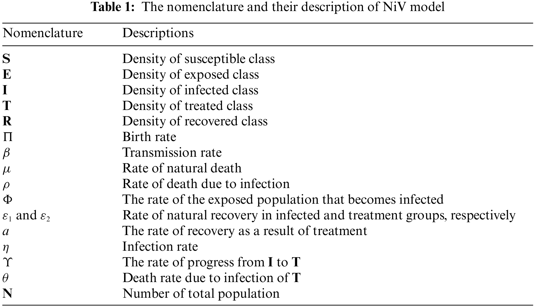
where various compartments, parameters and variables involved in the model are explained in the Table 1. Here, the total population of the community at time t is

Figure 1: Flow chart of the model (1)
Motivated by the importance of piecewise derivatives, we extend model (1) under the piecewise derivative with fractional order
Here, some basic results are recollected from fractional calculus.
Definition 3.1. [41]. The fractional derivative of
such that right hand side exists.
Definition 3.2. [41]. Fractional integration of
such that right hand side exists.
Definition 3.3. [24]. Let
with
Definition 3.4. Let
such that
Lemma 3.1. [24] The solution of
is given by
Some existence results are derived here. It should be kept in mind that prior to dealing with a dynamical system, existence theory is important to investigate for the prosed problem. As the model is used to estimate the population of humans, it is necessary that all of its parameters and variables for all time
Theorem 4.1. [33]. Let
Proof. By adding all equations of model (2), where
Take Laplace transform of and use
yields after simplification
After evaluating, we have
where
Also, it is straightforward to show that each compartment is non-negative.
Remark 1. Disease free equilibrium refers to a stable condition in which there is no infection or disease. The said point has been computed in [33] as
and the fundamental threshold number is given by
The said number predicts the transmission dynamics of disease in the community. If
Some 3D profiles of

Figure 2: 3D configuration of
Lemma 4.1. Inview of Lemma 3.1, the solution of
is given by
where
Proof. Following the fashion of Lemma 3.1, we can easily obtain the solution above. Let
We use the growth and Lipschtiz conditions on the non-linear operator
(D1) Let
(D2) If
Theorem 4.2. Let piece-wise continuous function
Proof. Using Schauder fixed point theorem, let denote a closed and bounded subset
Let
For
for
Thus, it proved that
By (7), we obtain
Since
It follows that
Next, we take the other interval
We see from (8), that
Hence,
Therefore,
Theorem 4.3. By hypothesis
Proof. Consider the mapping
Using (9), one has
For
From Eq. (11), we get
Therefore,
For piecewise derivable problem (2), we develop a numerical technique for the two sub-intervals of
The solution of (2) under the piecewise derivative can be expressed as
We will first develop the strategy for the first equation in System (12) and then apply it to the rest of the equations. At
Eq. (13) is expressed in the Newton interpolation formula given in the reference as
For the rest of three equations, we can write the Newton interpolation scheme as shown below:
and
6 Numerical Simulations and Discussion
We illustrate the numerical simulation in Figures utilizing the acquire scheme of Newton Polynomial of classical and global piece-wise derivative notion. We divide the interval into two sub-intervals and analyze the first for integer order derivatives, whereas the second is tested for different fractional orders in the sense of Caputo, using the data in a table. Here, we simulate our model corresponding to the numerical data given in Table 2. Here, we present approximate solutions under piecewise fractional order differentiation of the proposed model using various fractional orders. The concerned graphs for approximate solutions when
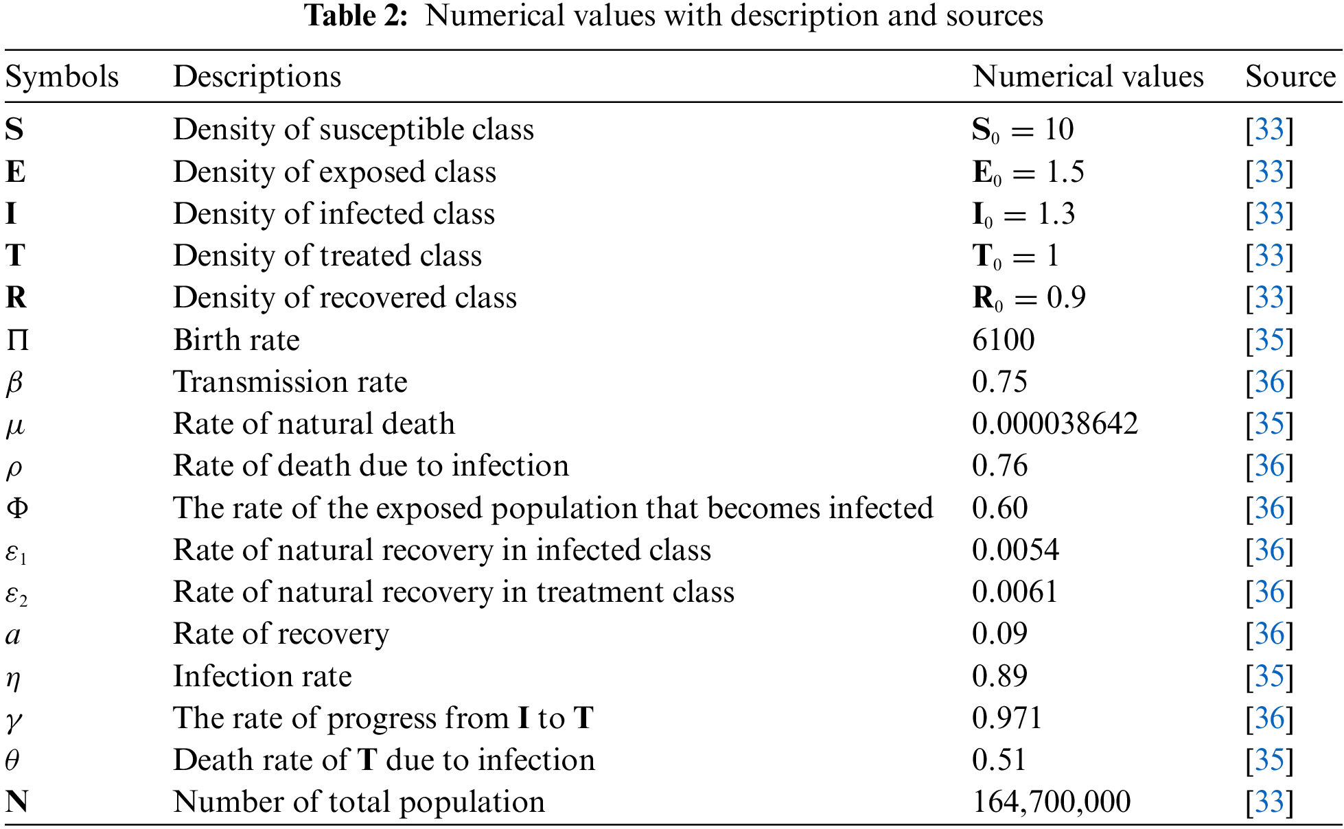
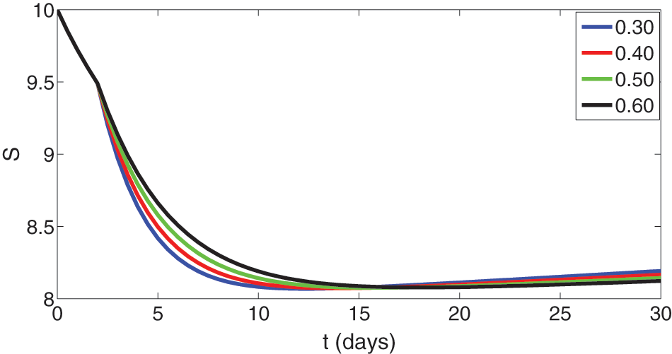
Figure 3: Graphical presentation of approximate solutions of susceptible compartment against different values of fractional orders such that

Figure 4: Graphical presentation of approximate solutions of exposed compartment against different values of fractional orders such that

Figure 5: Graphical presentation of approximate solutions of infected compartment against different values of fractional orders such that

Figure 6: Graphical presentation of approximate solutions of treated compartment against different values of fractional orders such that

Figure 7: Graphical presentation of approximate solutions of recovered compartment against different values of fractional orders such that

Figure 8: Graphical presentation of approximate solutions of susceptible compartment against different values of fractional orders such that

Figure 9: Graphical presentation of approximate solutions of exposed compartment against different values of fractional orders such that

Figure 10: Graphical presentation of approximate solutions of infected compartment against different values of fractional orders such that
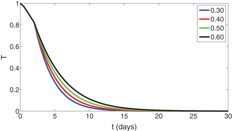
Figure 11: Graphical presentation of approximate solutions of treated compartment against different values of fractional orders such that

Figure 12: Graphical presentation of approximate solutions of recovered compartment against different values of fractional orders such that
In this article, we have developed a qualitative and computational analysis of a NiV disease. Based on the notion of the newly explored piecewise derivative of fractional order, we have investigated the model to study the crossover behavior in the dynamics of the disease. First of all, the invariance of the model and the feasible region has been established in the sense of the Caputo fractional derivative via using Laplace transform. Some remarks about thresholds number and their 3D profile corresponding to different parameters have been given. We have developed necessary and sufficient conditions for the existence and uniqueness of approximate solutions via fixed point results of Banach and Schauder. Utilizing the Newtonian polynomials of numerical interpolation, we have established algorithms for simulation purposes of the model. We have constructed the required scheme for numerical findings and their graphical presentation. We have simulated the model on different sets of fractional order by dividing the domain of time into two sub-intervals. Graphical presentations have indicated the crossover (multi-step) behavior in the dynamical study of the aforesaid model. In the future, this model can be investigated by using an ABC type derivative which has a nonlocal and nonsingular kernel. It would be expected that more dynamic properties may appear for better understanding.
Acknowledgement: The authors K. Shah, T. Abdeljawad, and B. Abdalla thank Prince Sultan University for support through the TAS Research Lab.
Funding Statement: The research was financially supported by Prince Sultan University.
Conflicts of Interest: The authors declare that they have no conflicts of interest to report regarding the present study.
References
1. Rizzardini, G., Saporito, T., Visconti, A. (2018). What is new in infectious diseases: Nipah virus, MERS-CoV and the blueprint list of the World Health Organization. Le Infezioni in Medicina, 26(3), 195–198. [Google Scholar]
2. Susilarini, N. K., Haryanto, E., Praptiningsih, C. Y., Mangiri, A., Kipuw, N. et al. (2018). Estimated incidence of influenza-associated severe acute respiratory infections in Indonesia, 2013–2016. Influenza and other Respiratory Viruses, 12(1), 81–87. DOI 10.1111/irv.12496. [Google Scholar] [CrossRef]
3. Zumla, A., David, S. C. H. (2019). Emerging and reemerging infectious diseases: Global overview. Infectious Disease Clinics, 33(4), xiii–xix. DOI 10.1016/j.idc.2019.09.001. [Google Scholar] [CrossRef]
4. Farrar, J. J. (1999). Nipah-virus encephalitis–investigation of a new infection. The Lancet, 354(9186), 1222–1223. DOI 10.1016/S0140-6736(99)90124-1. [Google Scholar] [CrossRef]
5. Chua, K. B., Bellini, W. J., Rota, P. A., Harcourt, B. H., Tamin, A. et al. (2000). Nipah virus: A recently emergent deadly paramyxovirus. Science, 288(5470), 1432–1435. DOI 10.1126/science.288.5470.1432. [Google Scholar] [CrossRef]
6. Nor, M., Gan, C. H., Ong, B. L. (2000). Nipah virus infection of pigs in peninsular Malaysia. Revue Scientifique et Technique (International Office of Epizootics), 19(1), 160–165. [Google Scholar]
7. Clayton, B. A., Middleton, D., Arkinstall, R., Frazer, L., Wang, L. F. et al. (2016). The nature of exposure drives transmission of Nipah viruses from Malaysia and Bangladesh in ferrets. PLoS Neglected Tropical Diseases, 10(6), e0004775. DOI 10.1371/journal.pntd.0004775. [Google Scholar] [CrossRef]
8. Bangyao, S., Jia, L., Liang, B., Chen, Q., Liu, D. (2018). Phylogeography, transmission, and viral proteins of Nipah virus. Virologica Sinica, 33(5), 385–393. DOI 10.1007/s12250-018-0050-1. [Google Scholar] [CrossRef]
9. Liew, Y., Ibrahim, P., Ong, H., Chong, C., Tan, C. et al. (2022). The immunobiology of Nipah virus. Microorganisms, 10(6), 1162. DOI 10.3390/microorganisms10061162. [Google Scholar] [CrossRef]
10. Sinha, D., Sinha, A. (2019). Mathematical model of zoonotic Nipah virus in South-East Asia region. Acta Scientific Microbiology, 2(9), 82–89. [Google Scholar]
11. World Health Organization (2018). List of blueprint priority diseases, R and D Blueprint: World Health Organization. [Google Scholar]
12. Nita, H. S., Niketa, D. T., Foram, A. T., Moksha, H. S. (2018). Control strategies for Nipah virus. International Journal of Applied Engineering Research, 13(21), 15149–15163. [Google Scholar]
13. Schountz, T. (2014). Immunology of bats and their viruses: Challenges and opportunities. Viruses, 6(12), 4880–4901. DOI 10.3390/v6124880. [Google Scholar] [CrossRef]
14. Monath, T. P., Nichols, R., Tussey, L., Scappaticci, K., Pullano, T. G. et al. (2022). Recombinant vesicular stomatitis vaccine against Nipah virus has a favorable safety profile: Model for assessment of live vaccines with neurotropic potential. PLoS Pathogens, 18(6), e1010658. DOI 10.1371/journal.ppat.1010658. [Google Scholar] [CrossRef]
15. Wang, Z., Amaya, M., Addetia, A., Dang, H. V., Reggiano, G. et al. (2022). Architecture and antigenicity of the Nipah virus attachment glycoprotein. Science, 375(6587), 1373–1378. DOI 10.1126/science.abm5561. [Google Scholar] [CrossRef]
16. Kapur, J. N. (1988). Mathematical modelling. New Delhi, India: New Age International. [Google Scholar]
17. Goh, K. J., Tan, C. T., Chew, N. K., Tan, P. S. K., Kamarulzaman, A. et al. (2000). Clinical features of Nipah virus encephalitis among pig farmers in Malaysia. New England Journal of Medicine, 342(17), 1229–1235. DOI 10.1056/NEJM200004273421701. [Google Scholar] [CrossRef]
18. Agarwal, P., Singh, R. (2020). Modelling of transmission dynamics of Nipah virus (NiVA fractional order approach. Physica A: Statistical Mechanics and its Applications, 547, 124243. DOI 10.1016/j.physa.2020.124243. [Google Scholar] [CrossRef]
19. Tan, K. S., Tan, C. T., Goh, K. J. (1999). Epidemiological aspects of Nipah virus infection. Neurology Asia, 4(1), 77–81. [Google Scholar]
20. Cross, R., Woolsey, C., Prasad, A., Borisevich, V., Agans, K. et al. (2022). A recombinant VSV-vectored vaccine rapidly protects nonhuman primates against lethal Nipah virus disease. Proceedings of the National Academy of Sciences, 119(12), e2200065119. DOI 10.1073/pnas.2200065119. [Google Scholar] [CrossRef]
21. Chong, H. T., Hossain, M. J., Tan, C. T. (2008). Differences in epidemiologic and clinical features of Nipah virus encephalitis between the Malaysian and Bangladesh outbreaks. Neurology Asia, 13, 23–26. [Google Scholar]
22. Hossain, M. J., Gurley, E. S., Montgomery, J. M., Bell, M., Carroll, D. S. et al. (2008). Clinical presentation of Nipah virus infection in Bangladesh. Clinical Infectious Diseases, 46(7), 977–984. DOI 10.1086/529147. [Google Scholar] [CrossRef]
23. Biswas, M. H. A. (2012). Model and control strategy of the deadly Nipah virus (NiV) infections in Bangladesh. Research and Reviews in Biosciences, 6(12), 370–377. [Google Scholar]
24. Atangana, A., Araz, S. I. (2021). New concept in calculus: Piecewise differential and integral operators. Chaos, Solitons & Fractals, 145, 110638. DOI 10.1016/j.chaos.2020.110638. [Google Scholar] [CrossRef]
25. Khan, M. A., Atangana, A. (2020). Modeling the dynamics of novel coronavirus (2019-nCov) with fractional derivative. Alexandria Engineering Journal, 59(4), 2379–2389. DOI 10.1016/j.aej.2020.02.033. [Google Scholar] [CrossRef]
26. Atangana, A. (2020). Modelling the spread of COVID-19 with new fractal-fractional operators: Can the lockdown save mankind before vaccination? Chaos, Solitons & Fractals, 136, 109860. DOI 10.1016/j.chaos.2020.109860. [Google Scholar] [CrossRef]
27. Atangana, A., Qureshi, S. (2019). Modeling attractors of chaotic dynamical systems with fractal-fractional operators. Chaos, Solitons & Fractals, 123, 320–337. DOI 10.1016/j.chaos.2019.04.020. [Google Scholar] [CrossRef]
28. Atangana, A., Igret Araz, S. (2021). Modeling and forecasting the spread of COVID-19 with stochastic and deterministic approaches: Africa and Europe. Advances in Difference Equations, 2021(1), 1–107. DOI 10.1186/s13662-021-03213-2. [Google Scholar] [CrossRef]
29. Veeresha, P., Ilhan, E., Prakasha, D. G., Baskonus, H. M., Gao, W. (2022). A new numerical investigation of fractional order susceptible-infected-recovered epidemic model of childhood disease. Alexandria Engineering Journal, 61(2), 1747–1756. DOI 10.1016/j.aej.2021.07.015. [Google Scholar] [CrossRef]
30. Omame, A., Sene, N., Nometa, I., Nwakanma, C. I., Nwafor, E. U. et al. (2021). Analysis of COVID-19 and comorbidity co-infection model with optimal control. Optimal Control Applications and Methods, 42(6), 1568–1590. DOI 10.1002/oca.2748. [Google Scholar] [CrossRef]
31. Yavuz, M., Sene, N. (2020). Stability analysis and numerical computation of the fractional predator-prey model with the harvesting rate. Fractal and Fractional, 4(3), 35. DOI 10.3390/fractalfract4030035. [Google Scholar] [CrossRef]
32. Evirgen, F. (2022). Transmission of Nipah virus dynamics under caputo fractional derivative. Journal of Computational and Applied Mathematics, 418, 114654. [Google Scholar]
33. Omede, B. I., Ameh, P. O., Omame, A., Bolaji, B. (2020). Modelling the transmission dynamics of Nipah virus with optimal control. arXiv preprint arXiv:2010.04111. [Google Scholar]
34. Mondal, M. K., Hanif, M., Biswas, M. H. A. (2017). A mathematical analysis for controlling the spread of Nipah virus infection. International Journal of Modelling and Simulation, 37(3), 185–197. DOI 10.1080/02286203.2017.1320820. [Google Scholar] [CrossRef]
35. Biswas, M. H. A., Haque, M. M., Duvvuru, G. (2015). A mathematical model for understanding the spread of Nipah fever epidemic in Bangladesh. International Conference on Industrial Engineering and Operations Management (IEOM), pp. 1–8. Dubai, United Arab Emirates. [Google Scholar]
36. Diekmann, O., Heesterbeek, J. A. P. (1989). Mathematical epidemiology of infectious diseases. New York: Wiley. [Google Scholar]
37. Shah, K., Abdeljawad, T., Abdalla, B., Abualrub, M. S. (2022). Utilizing fixed point approach to investigate piecewise equations with non-singular type derivative. AIMS Mathematics, 7(8), 14614–14630. DOI 10.3934/math.2022804. [Google Scholar] [CrossRef]
38. Zeb, A., Atangana, A., Khan, Z. A., Djillali, S. (2022). A robust study of a piecewise fractional order COVID-19 mathematical model. Alexandria Engineering Journal, 61(7), 5649–5665. DOI 10.1016/j.aej.2021.11.039. [Google Scholar] [CrossRef]
39. Kumlin, P. (2004). A note on fixed point theory. In: Functional analysis lecture. Chalmers & GU. https://www.studocu.com/sv/document/goteborgs-universitet/functional-analysis/lecture-notes-fixed-point-theory/839173. [Google Scholar]
40. Khastan, A., Nieto, J. J., Rodríguez-López, R. (2014). Schauder fixed-point theorem in semilinear spaces and its application to fractional differential equations with uncertainty. Fixed Point Theory and Applications, 2014(1), 1–14. [Google Scholar]
41. Kilbas, A. A., Srivastava, H. M., Trujillo, J. J. (2006). Theory and applications of fractional differential equations. Amester Dam: Elsevier. [Google Scholar]
42. Ramos, H. (2019). Formulation and analysis of a class of direct implicit integration methods for special second-order IVPs in predictor-corrector modes. In: Recent advances in differential equations and applications, pp. 33–61. New York. [Google Scholar]
Cite This Article
 Copyright © 2023 The Author(s). Published by Tech Science Press.
This work is licensed under a Creative Commons Attribution 4.0 International License , which permits unrestricted use, distribution, and reproduction in any medium, provided the original work is properly cited.
 Downloads
 Citation Tools