On a Novel Extended Lomax Distribution with Asymmetric Properties and Its Statistical Applications

1  Introduction

A brief state of the art of the Lomax (Lo) distribution, as well as some of its recent extensions, is necessary to appreciate the interest of our study. To begin, the Lo distribution has two parameters and can be viewed as a variant of the generalized Pareto distribution, commonly known as the Pareto of the second type (or type II). Mathematically speaking, it is defined by the following cumulative distribution function (cdf):

FLo(x;α,β)={1−(1+βx)−α,x>0,0,x≤0,(1)

where α>0 and β>0. Thus defined, α is a shape parameter and β is a scale parameter. The probability density function (pdf) is defined by

fLo(x;α,β)={αβ(1+βx)−α−1,x>0,0,x≤0,(2)

and the hazard rate function (hrf) is specified by

hLo(x;α,β)={αβ1+βx,x>0,0,x≤0,(3)

The Lo distribution has been used in a variety of ways in the literature. The authors in [1], for example, have widely used it for reliability modeling and life testing. When the data are heavily tailed, it has also been employed as an alternative to the exponential distribution (see [2]). The authors in [3] investigated the Lo distribution’s record values. Some recurrence links between the moments of record values from the Lo distribution were suggested in [4]. The authors in [5] investigated the order statistics of non-identical right-truncated Lo random variables. In addition, numerous scholars have explored the Lo model from a Bayesian perspective, see, for example, [6]. The authors in [7] proposed a Bayesian estimation of the Lo distribution’s survival function. The authors in [8] examined Lo distribution data that had been progressively type-II censored for competing risks. The authors in [9] have looked at the stress-strength model estimation problem for a Lo distribution based on general progressive-censored data. The authors in [10] discussed the Lo distribution’s uses in economics, actuarial modeling, queuing difficulties, and biological sciences. The Lo distribution has been extended in various ways, with various transformations adding one or more parameters. Among these extensions, we may mention the Marshall-Olkin extended Lo distribution in [11], later study on the statistical side in [12], the exponentiated Lo distribution in [13], beta Lo distribution in [14], Poisson Lo distribution in [15], exponential Lo distribution in [16], gamma Lo distribution in [17], Weibull Lo distribution in [18], beta exponentiated Lo distribution in [19], power Lo distribution in [20], exponentiated Weibull Lo distribution in [21], Weibull generalized Lo distribution in [22], Marshall-Olkin exponential Lo distribution in [23], type II Topp-Leone power Lo distribution in [24], Marshall-Olkin length biased Lo distribution in [25], Kumaraswamy generalized power Lo distribution in [26], odd Burr Lo distribution in [27], sine power Lo distribution in [28], Nadarajah-Haghighi Lo distribution in [29], new modified inverse Lo distribution in [30], Maxwell-Lo distribution in [31], minimum Lindley Lomax distribution in [32], new Weibull inverse Lo distribution in [33], and quasi-Poisson exponentiated exponential Lo distribution in [34].

In this article, we investigate a new extension of the Lo distribution, called the extended Lomax (ELo) distribution. It is defined by the following cdf:

FELo(x;α,β,λ)={1−(1+βx)−α[1+λαlog⁡(1+βx)],x>0,0,x≤0,(4)

where λ∈[0,1], α>0 and β>0. Alternatively, we can write this cdf as the following weighted expression:

FELo(x;α,β,λ)=1−[1−FLo(x;α,β)]w(x;α,β,λ),x∈R,(5)

where w(x;α,β,λ)={1+λαlog⁡(1+βx),x>0,0,x≤0,. When the parameters need to be explicit, we denote this distribution the ELo(α,β,λ) distribution. If we take λ=0, it is clear that the ELo distribution reduces to the Lo distribution introduced in [35]. Essentially, the ELo distribution extends the mathematical definition of the Lo distribution by modulating the positive logarithmic terms log⁡(1+βx) via the parameter λ. The presence of this logarithmic term and the additional parameter, λ, enhances the functional properties of the cdf of the Lo distribution. Some of the features of the ELo distribution that will be demonstrated later are listed below: (i) the ELo distribution is derived from a transformation of the log-weighted power (LP) distribution in [36], which supports the analytical definition of the weight function w(x;α,β,λ); (ii) The ELo distribution is found to be heavy-tailed, with a decreasing or unimodal pdf and a decreasing or upside-down bathtub hrf, i.e., the hrf as only one extremum and it is a maximum, both having diverse asymetrical shapes; these properties are required for a variety of modeling goals, including the fit of insurance claim data; (iii) the ELo distribution satisfies comprehensive first-order stochastic comparisons; (iv) the main moment and quantile measures are in closed-form, including important actuarial risk measures; (v) the parameters of the ELo distribution are estimable via standard statistical methods, and, last but not least; (vi) the ELo distribution can be used quite efficiently in concrete lifetime data analysis, and is especially efficient for those with a heavy tail. All these points will be developed in an in-depth manner in the study, illustrated by the means of numerical tables and graphics, when necessary.

The rest of the paper is as follows: Section 2 shows the functional details of the ELo distribution. Technical properties are provided in Section 3, including stochastic comparisons, moment properties, and quantile properties. Section 4 concerns an efficient parametric estimation strategy in the case where the parameters of the ELo distribution are unknown. Section 5 is devoted to the applications of the ELo distribution to insurance claims data with both goodness-of-fits and actuarial measures. A conclusion is provided in Section 6.

2  Extended Lomax Distribution

2.1 Some Distributional Remarks

The ELo distribution is defined by the cdf given by (4). We recall that, as introduced in [36], the LP distribution is defined by the following cdf:

FLP(x;α,λ)={1,x≥1,xα[1−λαlog⁡(x)],x∈(0,1),0,x≤0,(6)

with λ∈[0,1] and α>0. An overview of the LP distribution is as follows. The LP distribution is created by applying an original logarithmic weighted function to the cdf of the transmuted power (TP) distribution. It can be viewed as a straightforward modification of the log-Lindley distribution created in [37]. Its definition establishes a special stochastic ordering that includes power, transmuted power, and log-weighted power distributions. A large panel of decreasing and sharp (mesokurtic) increasing-decreasing shapes for the pdf and flexible bathtub shapes for the hrf are established. The LP distribution thus offers a statistical substitute for the TP distribution. This claim was also demonstrated practically; with the use of a standard estimation strategy, the LP model can offer a better fit than the TP model using real-life data sets.

The following result shows the link existing between the ELo and LP distribution.

Proposition 2.1. Let X be a random variable following the LP distribution. The random variable Y=(1/β)(X−1−1) with β>0 then follows the ELo distribution.

Proof. We proceed by using the cdfs of the involved random variables. Let us denote by FY(x) the cdf of Y. First, we notice that the domain of definition of Y is (0,+∞), implying that FY(x)=0 for x≤0. For x>0, we have

FY(x)=P(Y≤x)=P(1β(X−1−1)≤x)=P(X−1≤1+βx)=P(X≥(1+βx)−1)=1−FLP((1+βx)−1;α,λ)=1−(1+βx)−α[1+λαlog⁡(1+βx)].(7)

We recognize the cdf of the ELo distribution, ending the proof of the proposition.

2.2 Study of the cdf and pdf

First, let us investigate the asymptotic behavior of the cdf of the ELo distribution presented in Eq. (4). We have

FELo(x;α,β,λ)=αβx(1−λ+αβλx)(1+o(1))→0asx→0(8)

and, for λ∈(0,1],

FELo(x;α,β,λ)=1−λαβ−αx−αlog⁡(x)(1+o(1))→1asx→+∞.(9)

Since the asymptotic property 1−FELo(x;α,β,λ)=Cx−γ(1+o(1)) as x→+∞, where C>0 and γ>0, is not satisfied due to the presence of a logarithmic term log⁡(x), the ELo distribution has not a fat tail, contrary to the Lo distribution corresponding to the case λ=0. The rest of this part is devoted to the analysis of the pdf of the ELo distribution. First, it is specified by

fELo(x;α,β,λ)={αβ(1+βx)−α−1[1−λ+λαlog⁡(1+βx)],x>0,0,x≤0,(10)

Let us examine the analytical behavior of this function, beginning with the asymptotic behavior. We have

limx→0+fELo(x;α,β,λ)=αβ(1−λ).(11)

Thus, the parameter λ modulates the value of fELo(x;α,β,λ) at x=0; this value can be 0 for λ=1, which is not possible for the Lo distribution. For λ∈(0,1], we have

fELo(x;α,β,λ)=λα2β−αx−α−1log⁡(x)(1+o(1))→+∞asx→+∞.(12)

As a result, the right tail of the ELo distribution decreases with a “logarihtmic-polynomial” decay, which is slightly slower than the right tail of the Lo distribution.

The following proposition studies the mode properties of the ELo distribution.

Proposition 2.2.

•   For λ∈[0,(1+α)/(1+2α)], fELo(x;α,β,λ) is decreasing.

•   For λ∈((1+α)/(1+2α),1], fELo(x;α,β,λ) has only one extremum which is a maximum given as

x∗=1β(e[−α(1−2λ)−1+λ]/[λα(α+1)]−1).(13)

In this case, the ELo distribution is unimodal.

Proof. For x∈(0,1), the first derivative of fELo(x;α,β,λ) can be expressed as

fELo′(x;α,β,λ)=−αβ2(1+βx)−α−2[α(1−2λ)+1−λ+λα(α+1)log⁡(1+βx)].(14)

Therefore, for λ∈[0,(1+α)/(1+2α)], since the term in bracket is immediately positive, it is clear that fELo′(x;α,β,λ)<0, so fELo(x;α,β,λ) is decreasing. For λ∈[(1+α)/(1+2α),1], we have fELo′(x;α,β,λ)=0 if and only if x=x∗ as given in (13). This point is a maximum since fELo′(x;α,β,λ)>0 for x∈(0,x∗) and fELo′(x;α,β,λ)<0 for x∈(x∗,+∞). Thus x∗ is the mode of the ELo distribution, it is thus unimodal in this case.

It is clear that for any t>0, we have ∫0+∞etxfELo(x;α,β,λ)dx=+∞; the ELo distribution is heavy-tailed (but it is not fat-tailed, as previously shown).

Fig. 1 illustrates the mathematical result aboves by displaying several plots of fELo(x;α,β,λ).

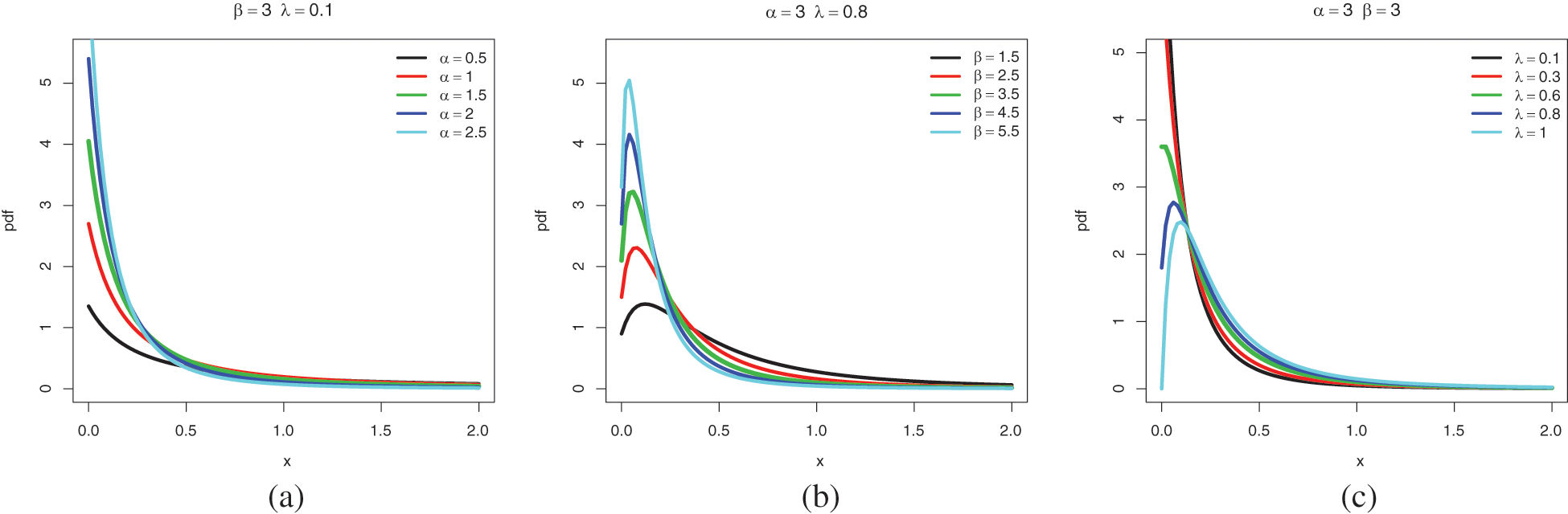
Figure 1: Plots of the pdf of the ELo distribution for the following sets of values: (a) β=3, λ=0.1 and α∈{0.5,1,1.5,2,2.5}, (b) α=3, λ=0.8 and β∈{1.5,2.5,3.5,4.5,5.5}, and (c) α=3, β=3 and λ∈{0.1,0.3,0.6,0.8,1}

As expected, fELo(x;α,β,λ) has decreasing or unimodal asymetrical shapes, with varying weights on the left tail and the right tail remaining more or less heavy depending on the values of the parameters. The functional possibilities of the Lo distribution are overpassed, as demonstrated in Fig. 2, where the unimodal shapes are totally abscent.

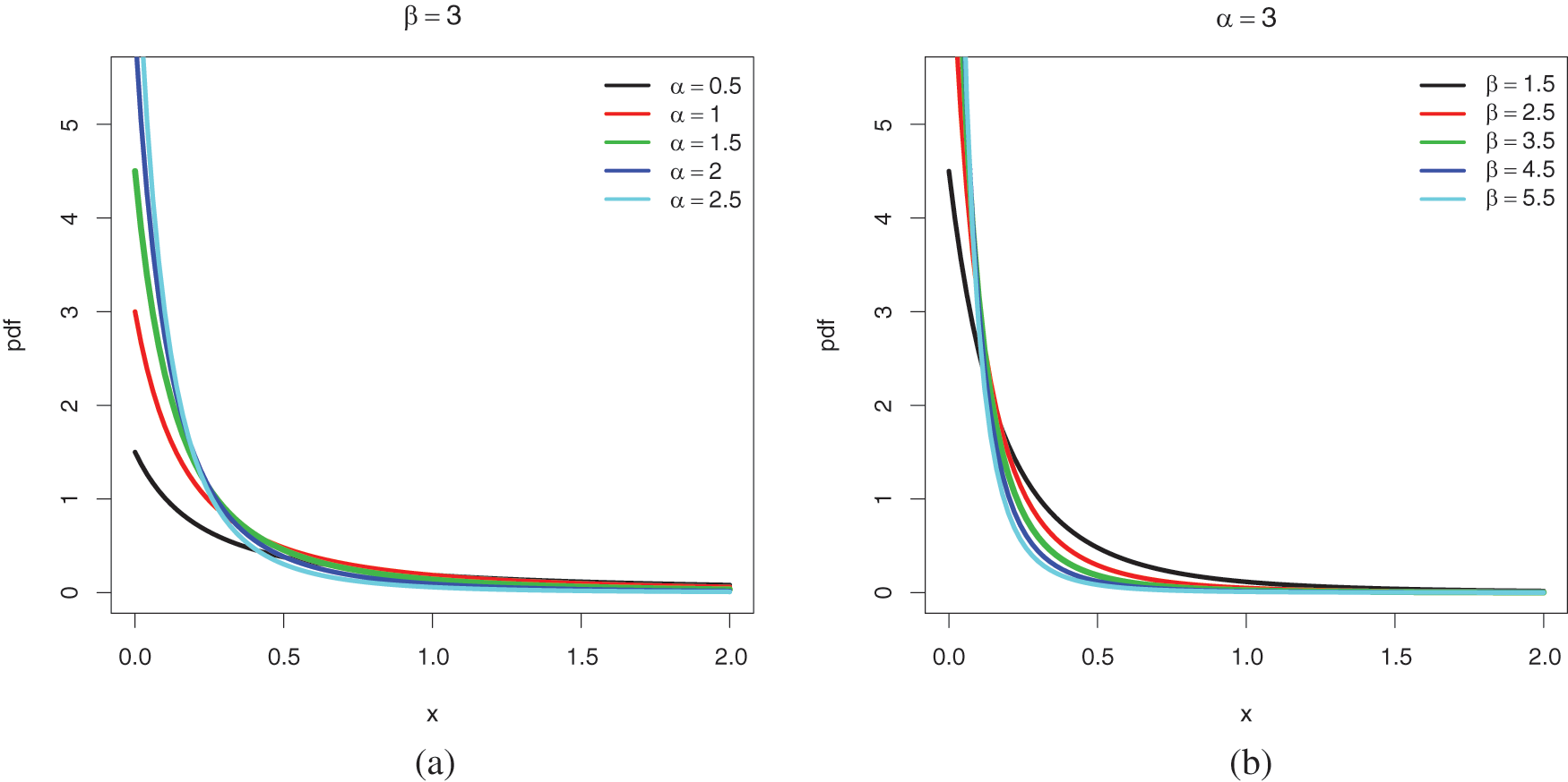
Figure 2: Recall of some plots of the pdf of the Lo distribution for the following sets of values: (a) β=3 and α∈{0.5,1,1.5,2,2.5}, and (b) α=3 and β∈{1.5,2.5,3.5,4.5,5.5}

Now, consider the ratio function fELo(x;α,β,λ)/fLo(x;α,β) for a more in-depth comparison of the pdfs of the ELo and Lo distributions. We have

fELo(x;α,β,λ)fLo(x;α,β)=1−λ+λαlog⁡(1+βx).(15)

Therefore, for λ∈(0,1], if x∈(0,(e1/α−1)/β), then we have fELo(x;α,β,λ)<fLo(x;α,β), and of x>(e1/α−1)/β, we have fELo(x;α,β,λ)>fLo(x;α,β). As a result, x∗=(e1/α−1)/β can be regarded as a transition point between the ELo and Lo distributions.

2.3 Study of the hrf

The hrf of the ELo distribution is defined by

hELo(x;α,β,λ)={αβ1−λ+λαlog⁡(1+βx)(1+βx)[1+λαlog⁡(1+βx)],x>0,0,x≤0,(16)

The following limit holds:

limx→0+hELo(x;α,β,λ)=αβ(1−λ).(17)

The remarks made on fELo(x;α,β,λ) when x→0+ are still valid here; the parameter λ has a non-negligible effect on the initial value of hELo(x;α,β,λ), can be equal to 0. We have

hELo(x;α,β,λ)=αβ1+βx(1+o(1))→0asx→+∞.(18)

Thus, for all the configurations of the parameters, the hrf decays to 0 with a polynomial rate.

The shape behavior of the hrf is studied in the next proposition.

Proposition 2.3.

•   For λ∈[0,2/(1+4α+1)], hELo(x;α,β,λ) is decreasing.

•   For λ∈(2/(1+4α+1),1], hELo(x;α,β,λ) has only one extremum which is a maximum given as

x∗=1β(e(λ−2+λ4α+1)/(2αλ)−1).(19)

In this last case, the shape of hELo(x;α,β,λ) is upside-down bathtub.

Proof. We have

hELo′(x;α,β,λ)=−αβ2P[αλlog⁡(1+βx)](1+βx)2[1+λαlog⁡(1+βx)]2.(20)

where

P(u)=u2+(2−λ)u−αλ2+1−λ,u>0.(21)

Then the polynomial P(u) has two roots given by

u1=12(λ−2−λ4α+1),u2=12(λ−2+λ4α+1)(22)

and we have P(u)=(u−u1)(u−u2). Since λ∈[0,1], we always have u1<0. Therefore, if u2≤0, i.e., λ∈[0,2/(1+4α+1)], we have P(u)>0 for all u>0, implying that hELo′(x;α,β,λ)<0, so hELo(x;α,β,λ) is decreasing. If u2≥0, i.e., λ∈(2/(1+4α+1),1], u2 is a valid root for P(u), and thus hELo′(x∗;α,β,λ)=0 if and only if αλlog⁡(1+βx∗)=u2, so

x∗=1β(eu2/(αλ)−1),(23)

which can be expressed as (19). This point is a maximum since hELo′(x;α,β,λ)>0 for x∈(0,x∗) and hELo′(x;α,β,λ)<0 for x∈(x∗,+∞). Hence, the shape of hELo(x;α,β,λ) is upside-down bathtub. This ends the proof.

Fig. 3 provides various plots of hELo(x;α,β,λ) to demonstrate the above mathematical result.

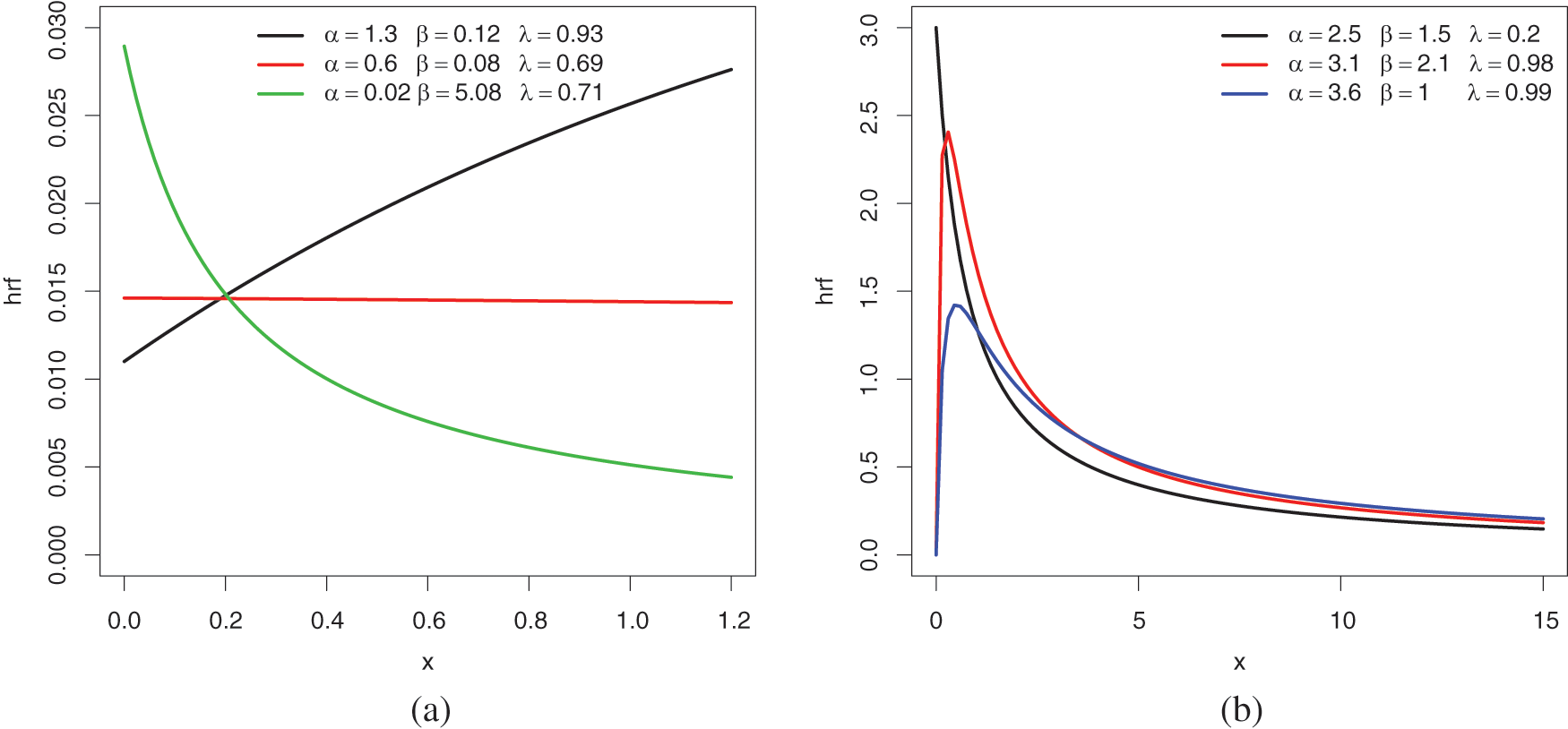
Figure 3: Plots of the hrf of the ELo distribution for the following sets of values: (a) (α,β,λ)∈{(1.3,0.12,0.93),(0.6,0.08,0.69),(0.02,5.08,0.71)} and (b) (α,β,λ)∈{(2.5,1.5,0.2),(3.1,2.1,0.98),(3.6,1,0.99)}

The UBFR property is particularly illustrated in Fig. 3b. For modeling purposes in the analysis of financial, survival, and environmental data, this is a desired property of the heavy-tailed distribution. We recall that the UBR property is not a quality of the Lo distribution, as shown in Fig. 4.

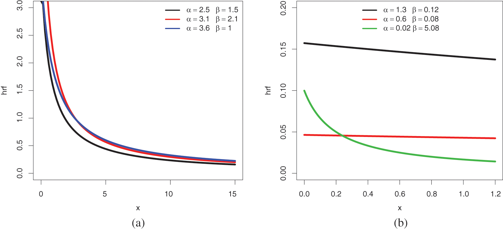
Figure 4: Recall of some plots of the hrf of the Lo distribution for the following sets of values: (a) (α,β)∈{(2.5,1.5),(3.1,2.1),(3.6,1} and (b) (α,β)∈{(1.3,0.12),(0.6,0.08),(0.002,5.08)}

3  Technical Properties

Some technical properties of the ELo distribution are now examined.

3.1 Stochastic Comparisons

Following the approach presented in [38], we now study certain stochastic ordering aspects of the ELo distribution.

Proposition 3.1. The following first-order stochastic (FOS) comparisons hold:

•   For α2≥α1, the ELo (α1,β,λ) distribution FOS dominates the ELo (α2,β,λ) distribution; it is understood that the dominance is strict for α2>α1, with equality if and only if α2=α1.

•   For β2≥β1, the ELo (α,β1,λ) distribution FOS dominates the ELo (α,β2,λ) distribution.

•   For λ2≥λ1, the ELo (α,β,λ2) distribution FOS dominates the ELo (α,β,λ1) distribution. In particular, the ELo (α,β,λ) distribution FOS dominates the Lo distribution with parameters α and β.

Proof. We proceed by studying the monotonicity of FELo(x;α,β,λ) according to the parameters.

•   For x>0, we have

∂∂αFELo(x;α,β,λ)=(1+βx)−αlog⁡(1+βx)[1−λ+λαlog⁡(1+βx)].(24)

Since λ∈[0,1], we have ∂FELo(x;α,β,λ)/(∂α)≥0, so FELo(x;α,β,λ) is increasing with respect to α. Thus, for α2≥α1, we have FELo(x;α1,β,λ)≤FELo(x;α2,β,λ), meaning that the ELo(α1,β,λ) distribution FOS dominates the ELo(α2,β,λ) distribution.

•   For x>0, we have

∂∂βFELo(x;α,β,λ)=αx(1+βx)−α−1[1−λ+λαlog⁡(1+βx)].(25)

Since λ∈[0,1], we have ∂FELo(x;α,β,λ)/(∂β)≥0, so FELo(x;α,β,λ) is increasing with respect to β. Thus, for β2≥β1, we have FELo(x;α,β1,λ)≤FELo(x;α,β2,λ), meaning that the ELo(α,β1,λ) distribution FOS dominates the ELo(α,β2,λ) distribution. An alternative proof can be made for this point by using Proposition 2.1.

•   For x>0, we have

∂∂λFELo(x;α,β,λ)=−(1+βx)−αlog⁡(1+βx)(26)

It is clear that ∂FELo(x;α,β,λ)/(∂λ)≤0, so FELo(x;α,β,λ) is decreasing with respect to λ. Thus, for λ2≥λ1, we have FELo(x;α,β,λ2)≤FELo(x;α,β,λ1), meaning that the ELo(α,β,λ2) distribution FOS dominates the ELo(α,β,λ1) distribution. By taking λ2=λ and λ1=0, we conclude that the ELo(α,β,λ) distribution FOS dominates the Lo distribution with parameters α and β.

This ends the proof.

Thanks to Proposition 3.1, we now see how random values from the ELo distribution can be relatively located in comparison to other random values of the ELo distribution with different parameters. This could be useful in cases where the practitioner is unsure which ELo distribution to employ while dealing with data. For further details on stochastic dominance, we may refer to [39–40].

3.2 Moment Properties

Because they can be used to explain statistical distribution properties, moment properties are important when specifying our probability distribution to work with. As a result, they help to describe the distribution. In this part, different types of moments of the ELo distribution are examined, along with their interpretation.

Hereafter, we designate by X a random variable with the ELo distribution. The following result suggests a clear and simple finite sum expression for the rth moment of X.

Proposition 3.2. For any integer r<α−2, the rth moment of X exists, and it is given by mr=E(Xr), where E stands for the expectation operator. It can be expressed by a finite sum as

mr=rβr∑k=0r−1(r−1k)(−1)r−1−kα−k−1[1+λαα−k−1].(27)

Proof. Since the ELo distribution has the support (0,+∞), we have

mr=r∫0+∞xr−1[1−FELo(x;α,β,λ)]dx=r∫0+∞xr−1(1+βx)−α[1+λαlog⁡(1+βx)]dx.(28)

By performing the change of variable x=(1/β)(y−1) and applying the standard binomial formula, by noticing that α−k−1≥α−r−2>0 for k=0,…,r−1, we obtain

E(Xr)=rβr∫1+∞(y−1)r−1y−α[1+λαlog⁡(y)]dy=rβr∑k=0r−1(r−1k)(−1)r−1−k∫1+∞yk−α[1+λαlog⁡(y)]dy=rβr∑k=0r−1(r−1k)(−1)r−1−k[1α−k−1+λα∫1+∞yk−αlog⁡(y)dy].(29)

For the remaining integral term, upon the change of variable y=eu/(α−k−1), since ∫0+∞ue−udu=Γ(2)=1, we have

∫1+∞yk−αlog⁡(y)dy=1(α−k−1)2∫0+∞ue−udu=Γ(2)(α−k−1)2=1(α−k−1)2.(30)

Therefore, by combining the above equalities, we get

mr=rβr∑k=0r−1(r−1k)(−1)r−1−kα−k−1[1+λαα−k−1].(31)

The stated result is obtained, ending the proof.

It is worth noting from Proposition 3.2 that the ELo distribution does not admit moments of all orders.

In particular, according to Proposition 3.2, for α>4, the two first moments of X are given by

m1=1(α−1)β(1+λαα−1)(32)

and

m2=2β2[−1α−1(1+λαα−1)+1α−2(1+λαα−2)]=2(2α2λ+α2−3αλ−3α+2)β2(α−2)2(α−1)2.(33)

Similarly, Proposition 3.2 allows the variance, moments skewness and kurtosis of X to be expressed in terms of α, β and λ, but they lack an especially interesting concise form.

Among the possible generalizations of the moments are the unconditional moments, which naturally appear in various survival measures and are more suitable for use in a practical setting with censored data. On this topic, we may refer to [41,42].

The next result expresses the rth unconditional moment of X at a fixed value t.

Proposition 3.3. For any integer r and fixed t>0, the rth unconditional moment of X at a fixed value t exists, and is given by mr(t)=E(Xr∣X≤t). Under the condition that r<α−2, it can be expressed as

mr(t)=11−(1+βt)−α[1+λαlog⁡(1+βt)]×{−tr(1+βt)−α[1+λαlog⁡(1+βt)]+rβr∑k=0r−1(r−1k)(−1)r−1−kα−k−1[1−(1+βt)k−α+1+λαγ(2,log⁡[(α−k−1)(1+βt)])α−k−1]},(34)

where γ(a,x)=∫0xta−1e−tdt is the standard incomplete gamma function.

Proof. We have

mr(t)=1FELo(t;α,β,λ)∫0txrfELo(x;α,β,λ)dx.(35)

For t>0, we have FELo(t;α,β,λ)=1−(1+βt)−α[1+λαlog⁡(1+βt)], and an integration by part yields

∫0txrfELo(x;α,β,λ)dx=−tr[1−FELo(t;α,β,λ)]+r∫0txr−1[1−FELo(x;α,β,λ)]dx=−tr(1+βt)−α[1+λαlog⁡(1+βt)]+r∫0txr−1(1+βx)−α[1+λαlog⁡(1+βx)]dx.(36)

By performing the change of variable x=(1/β)(y−1) and applying the standard binomial formula, we get

∫0txr−1(1+βx)−α[1+λαlog⁡(1+βx)]dx=1βr∫11+βt(y−1)r−1y−α[1+λαlog⁡(y)]dy=1βr∑k=0r−1(r−1k)(−1)r−1−k∫11+βtyk−α[1+λαlog⁡(y)]dy=1βr∑k=0r−1(r−1k)(−1)r−1−k[1−(1+βt)k−α+1α−k−1+λα∫11+βtyk−αlog⁡(y)dy].(37)

For the remaining integral term, by using the incomplete gamma function and doing the change of variable y=eu/(α−k−1), we obtain

∫11+βtyk−αlog⁡(y)dy=1(α−k−1)2∫0log⁡[(α−k−1)(1+βt)]ue−udu=γ(2,log⁡[(α−k−1)(1+βt)])(α−k−1)2.(38)

Therefore, by combining the above equalities, we get

mr(t)=11−(1+βt)−α[1+λαlog⁡(1+βt)]×{−tr(1+βt)−α[1+λαlog⁡(1+βt)]+rβr∑k=0r−1(r−1k)(−1)r−1−kα−k−1[1−(1+βt)k−α+1+λαγ(2,log⁡[(α−k−1)(1+βt)])α−k−1]}.(39)

The stated result is obtained, ending the proof of Proposition 3.3.

Based on the conditional moments, we can define the moments of the residual life of the ELo distribution, and the mean residual life (MRL) function in particular. We can refer to [43–45] to support the importance of this last function in various branches of probability and statistics.

3.3 Quantile Properties

Because the ELo distribution does not admit moments of all orders, its quantile properties are fascinating to investigate.

The next result is a closed-form expression for the quantile function (qf) of the ELo distribution.

Proposition 3.4. The qf of the ELo distribution is expressed as

QELo(u;α,β,λ)={1β[(1−u)−1/α−1]forλ=0,1β[{λu−1W[u−1λe−1/λ]}1/α−1]forλ∈(0,1],u∈(0,1),(40)

where W(x) denotes the Lambert function, i.e., satisfying the equation W(x)eW(x)=x.

Proof. The qf is readily defined as QELo(u;α,β,λ)=FELo−1(u;α,β,λ). Thus, we determine it via the following equivalences: For λ>0, we have

1−(1+βx)−α[1+λαlog⁡(1+βx)]=u⇔(1+βx)−α[1+λαlog⁡(1+βx)]=1−u⇔log⁡[(1+βx)α]=1λ[(1−u)(1+βx)α−1]⇔(1+βx)α=e−1/λe(1−u)(1+βx)α/λ⇔u−1λ(1+βx)αe(u−1)(1+βx)α/λ=u−1λe−1/λ⇔u−1λ(1+βx)α=W[u−1λe−1/λ]⇔x=1β[{λu−1W[u−1λe−1/λ]}1/α−1].(41)

The desired expression is established, ending the proof of Proposition 3.4.

There are several interests in having a closed-form expression of the qf. First of all, the main quartiles of the ELo distribution can be exhibited. In particular, the median is obtained as

M=QELo(12;α,β,λ)={1β(21/α−1)forλ=0,1β[{−2λW[−12λe−1/λ]}1/α−1]forλ∈(0,1].(42)

The qf and random values from the uniform distribution over [0, 1] can be used to generate random values from a random variable X following the ELo distribution.

Since the ELo distribution does not admit moments of all orders, quantile measures of skewness and kurtosis, as proposed in [46,47] respectively can be useful. They are respectively defined as

SGalton=QELo(6/8;α,β,λ)−2QELo(4/8;α,β,λ)+QELo(2/8;α,β,λ)QELo(6/8;α,β,λ)−QELo(2/8;α,β,λ),(43)

and

KMoors=QELo(7/8;α,β,λ)−QELo(5/8;α,β,λ)+QELo(3/8;α,β,λ)−QELo(1/8;α,β,λ)QELo(6/8;α,β,λ)−QELo(2/8;α,β,λ).(44)

In our heavy-tailed distribution setting, we propose to focus on actuarial measures based on the qf. The first measure is the value at risk (VaR). In the setting of the ELo distribution, it is simply defined by

VaRq=QELo(q;α,β,λ),q∈(0,1).(45)

The second mesure is the expected shortfall (ES) introduced by [48], and generally considered as a better measure than VaR. It is defined by

ESq=1q∫0qVaRxdx,q∈(0,1).(46)

Fig. 5 presents the shape of these actual measures for various values of the parameters with respect to q.

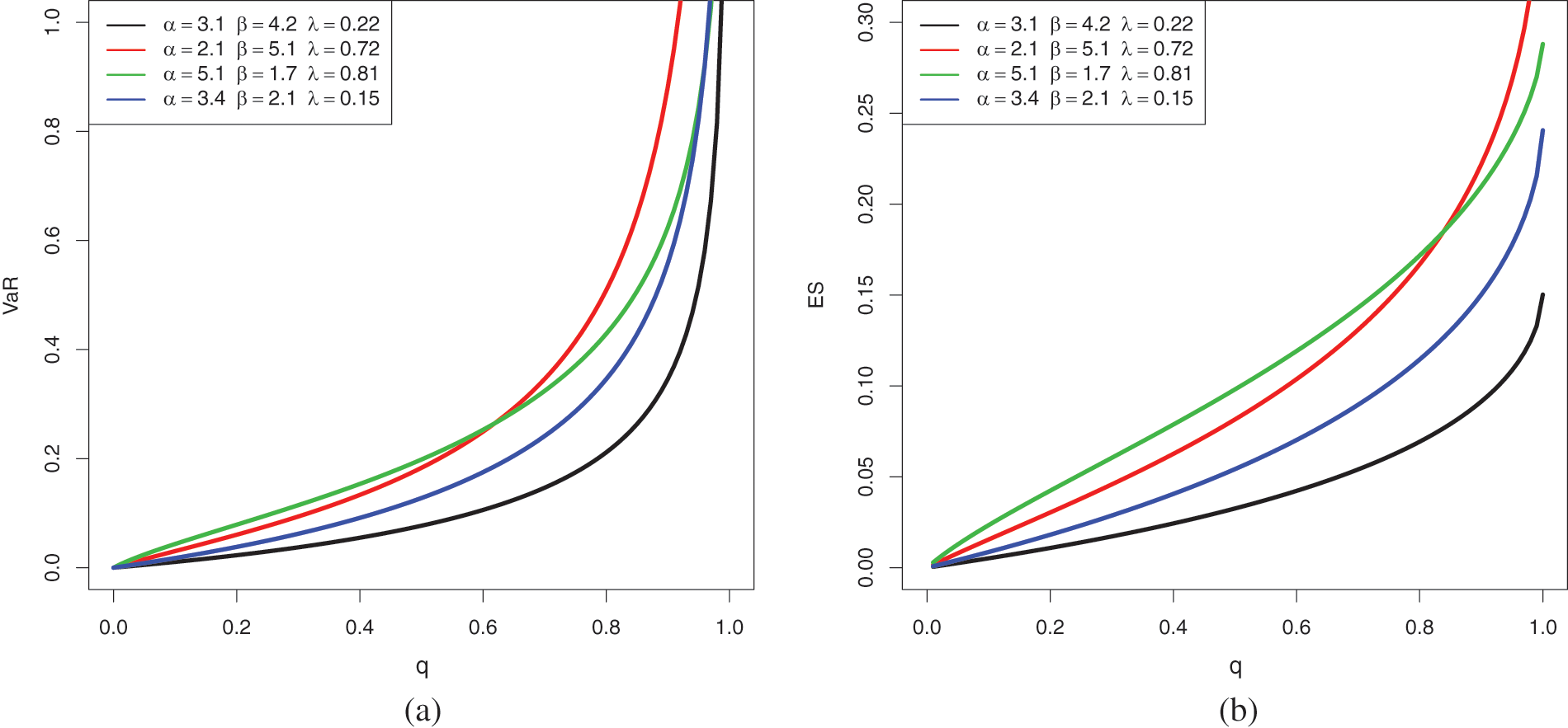
Figure 5: Plots of (a) VaRq and (b) ESq for the ELo distribution for various values of the parameters and q∈(0,1)

According to Fig. 5, both VaRq and ESq are increasing and convex, with a more or less angular shape.

In addition to the above quantile material, advanced quantile modeling can be done using the qf. See [49] for further details.

4  Estimation

We now want to estimate the unknown parameters α, β, and λ in the ELo distribution using data that can be logically fitted with this distribution. To do so, we employ the maximum likelihood (ML) method for complete samples. We describe it in detail below, and perform a simulated experiment on the obtained estimates.

4.1 Method

Let x1,…,xn represent n independent observations from a random variable X following the ELo(α,β,λ) distribution. Then, based on the pdf specified by (10) and x=(x1,…,xn), the likelihood function is specified by

L(α,β,λ;x)=∏i=1nfELo(xi;α,β,λ)=∏i=1nαβ(1+βxi)−α−1[1−λ+λαlog⁡(1+βxi)].(47)

Clearly, the ELo distribution does not belong to the exponential family form; the Pitman-Koopman theorem applies. The ML estimates (MLEs) of α and λ are given by

(α^,β^,λ^)=argmax(α,β,λ)L(α,β,λ;x).(48)

Alternatively, they may be defined as

(α^,β^,λ^)=argmax(α,β,λ)ℓ(α,β,λ;x),(49)

where ℓ(α,λ;x) refers to the log-likelihood function given by

ℓ(α,β,λ;x)=log⁡[L(α,β,λ;x)]=nlog⁡(α)+nlog⁡(β)−(α+1)∑i=1nlog⁡(1+βxi)+∑i=1nlog⁡[1−λ+λαlog⁡(1+βxi)].(50)

They can be obtained by solving the following non-linear equations with respect to α and λ

∂ℓ(α,β,λ;x)∂α=0,∂ℓ(α,β,λ;x)∂β=0,∂ℓ(α,β,λ;x)∂λ=0,(51)

where

∂ℓ(α,β,λ;x)∂α=nα−∑i=1nlog⁡(1+βxi)+∑i=1nλlog⁡(1+βxi)1−λ+λαlog⁡(1+βxi),(52)

∂ℓ(α,β,λ;x)∂β=nβ−(α+1)∑i=1nxi1+βxi+∑i=1nλαxi(1+βxi)|1−λ+λαlog⁡(1+βxi)](53)

and

∂ℓ(α,β,λ;x)∂λ=∑i=1nαlog⁡(1+βxi)−11−λ+λαlog⁡(1+βxi).(54)

Unfortunately, because the above equations have no explicit solutions, any numerical approximation technique can be utilized to obtain them. The related standard errors (SEs) can be determined through the calculation of the estimated Fisher information matrix. To accomplish the above calculations, the AdequacyModel package in R−Statistical\ Computing\ Environment can be used.

The ML method has the advantage of ensuring interesting features for MLEs, such as asymptotic unbiasedness and normality. In particular, the asymptotic unbiasedness provides theoretical guarantees on the fact that, for n large enough, the MLEs must be close to the true unknown parameter values. However, there is no solid guarantee for small n. The asymptotic normality allows us to construct confidence intervals and statistical tests on the unknown parameters based on the normal or normal-transformaiton distribution [50]. Contains more information about these features. We can estimate all of the underlying functions of the ELo distribution using MLEs. In particular, an estimate of the cdf and pdf are given by F^ELo(x)=F(x;α^,β^,λ^) and f^ELo(x)=f(x;α^,β^,λ^), respectively. With the same substitution approach, one can estimate various measures, such as the actuarial measures as defined in (45) and (46).

The above methodology is for complete samples. Other types of samples, such as censored data samples, can be investigated with appropriate modifications to the definition of the likelihood function. On this topic, we may refer the reader to [7,8,11,51].

The rest of this section is devoted to simulated tests proving the nice behavior of the MLEs.

4.2 Simulation Study

We carry out a Monte Carlo simulation study in order to underline the accuracy of the MLEs parameters of the ELo distribution. To this end, N=600 samples are considered at varying sample sizes, chosen as: n=20,40,…,600 for the following parameter value scenarios: Set 1: (α=1,β=1.5,λ=0.2), Set 2: (α=1.5,β=0.5,λ=0.2), and Set 3: (α=2,β=0.5,λ=0.1). The average MLEs are calculated, as well as the bias and the mean squared error (MSE) defined by

Bias(θ^)=∑i=1600θi^600−θ,MSE(θ^)=∑i=1600(θi^−θ)2600,(55)

respectively, where θ∈{α,β,λ}, and the index i refers to the ith sample for the given sample size. The detailed summary of the simulation is depicted in Tables 1–3 for Sets 1, 2 and 3, respectively. For a visual approach, the corresponding plots are given in Figs. 6–8, respectively, with n in absisse.

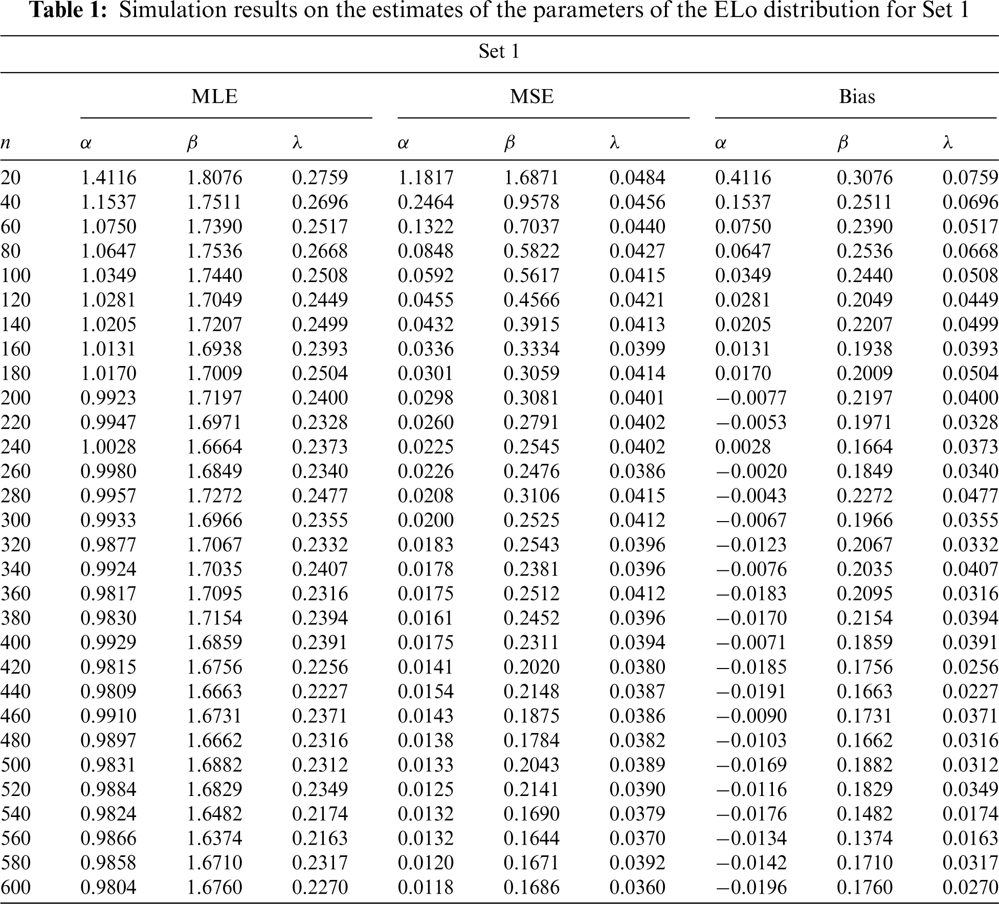
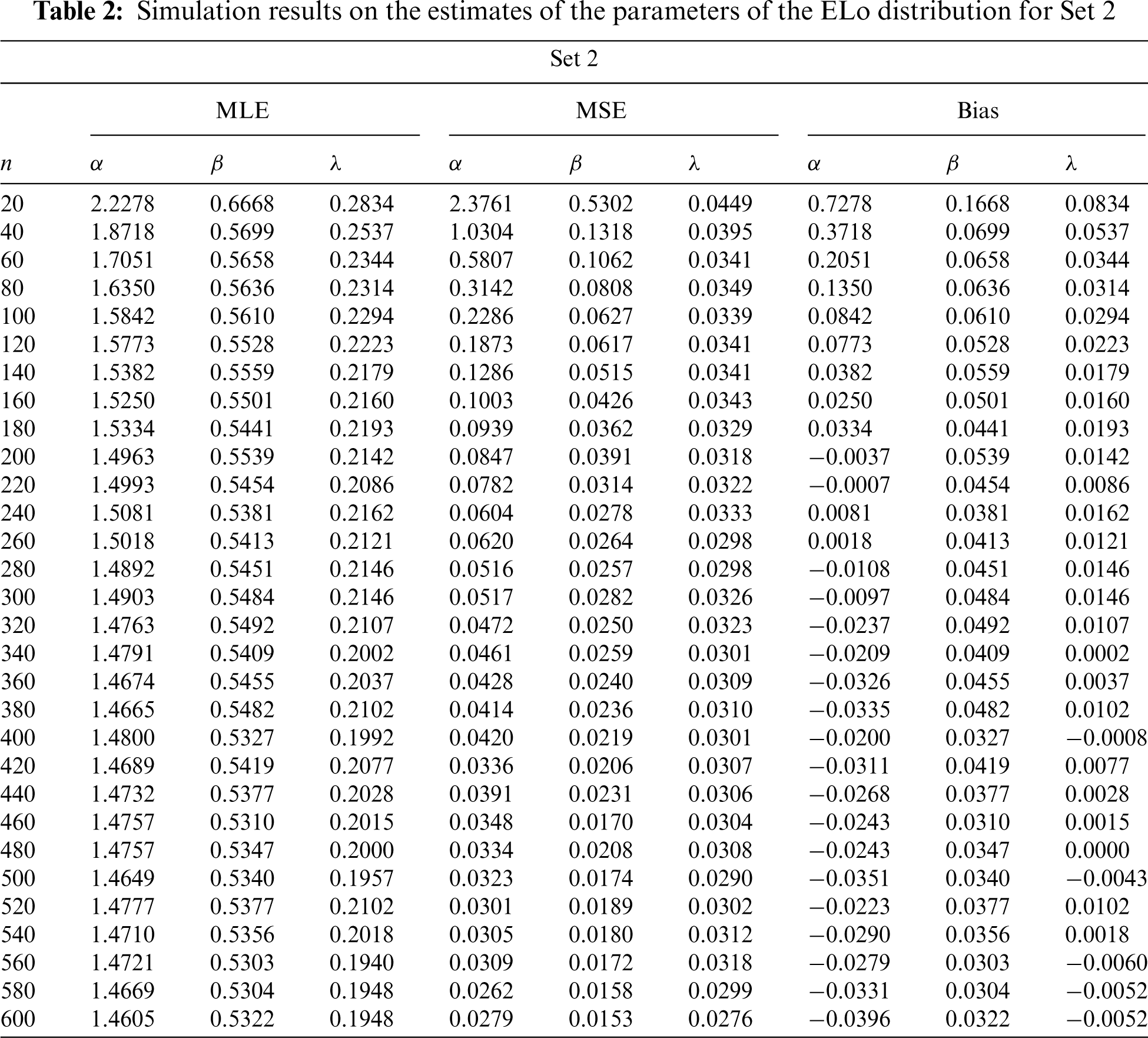
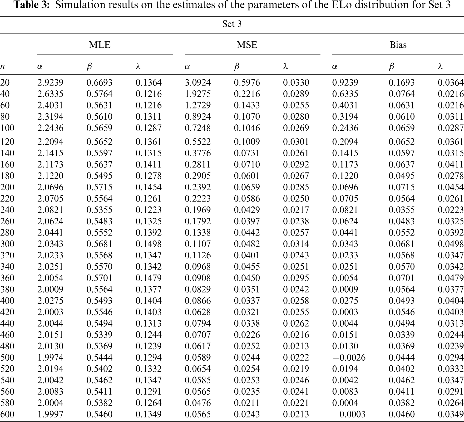
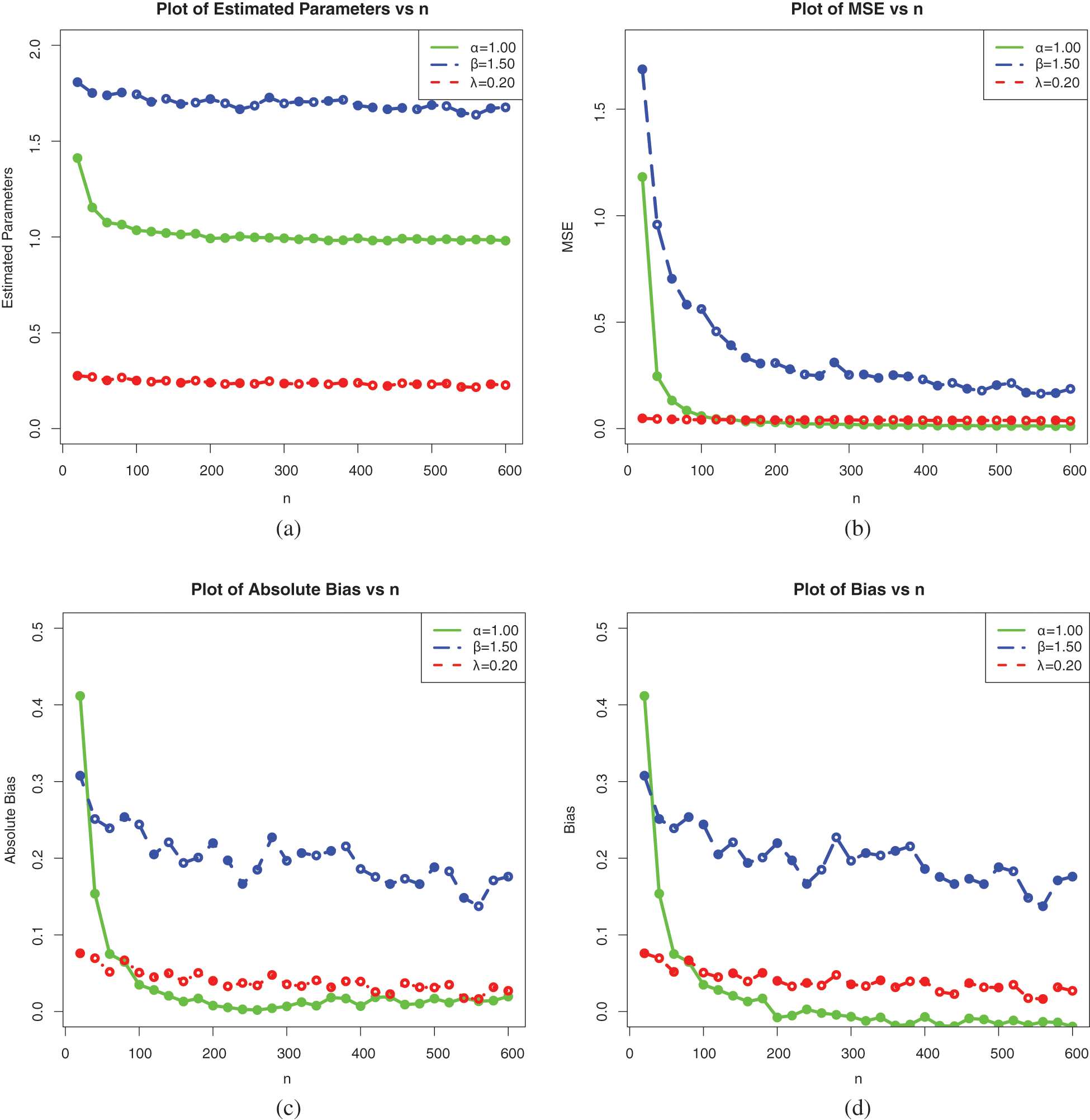
Figure 6: Plots of the simulation results on the estimates of the parameters of the ELo distribution for Set 1: (a) Average MLEs, (b) MSEs, (c) Absolute biases and (d) Biases

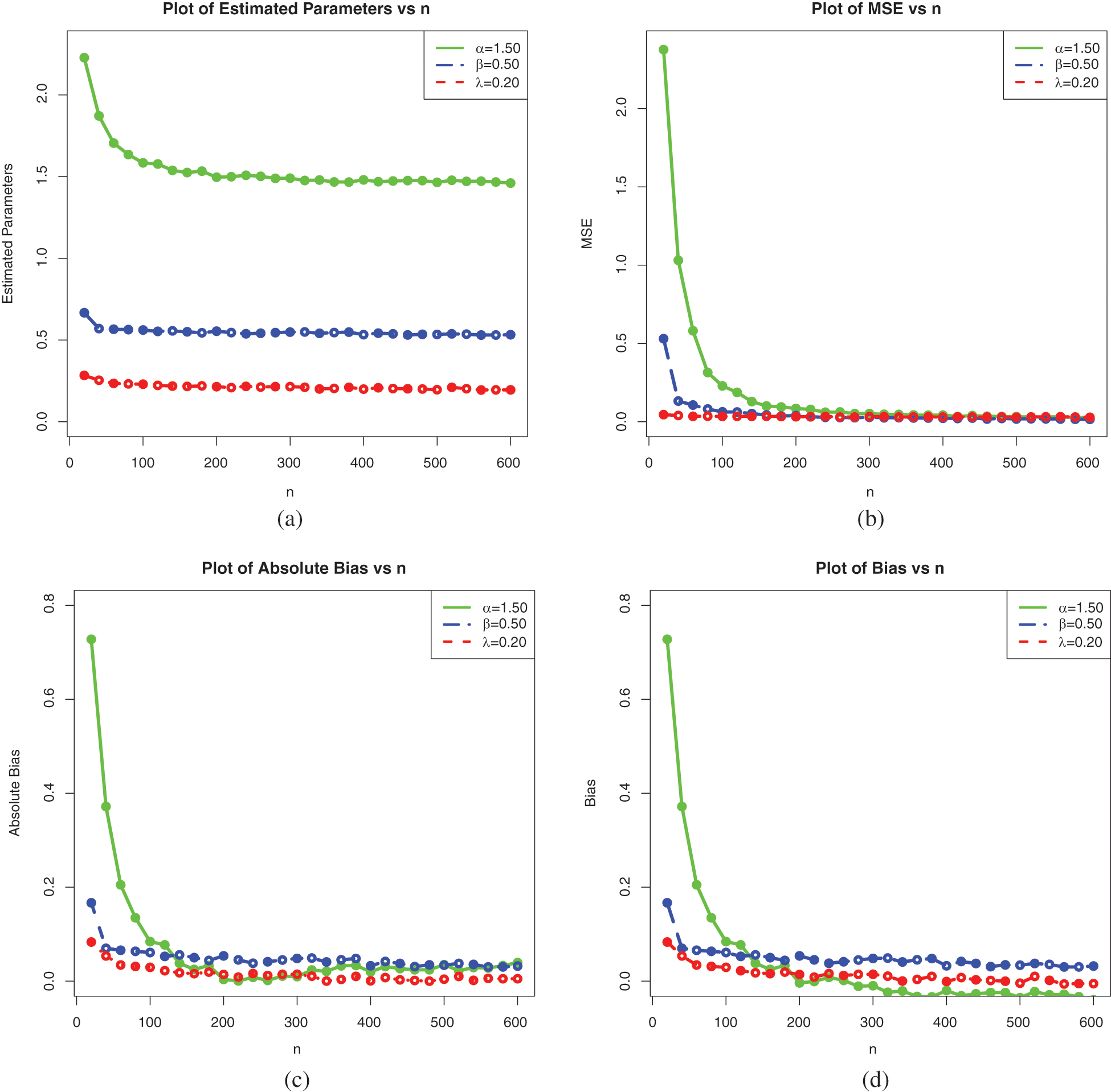
Figure 7: Plots of the simulation results on the estimates of the parameters of the ELo distribution for Set 2: (a) Average MLEs, (b) MSEs, (c) Absolute biases and (d) Biases

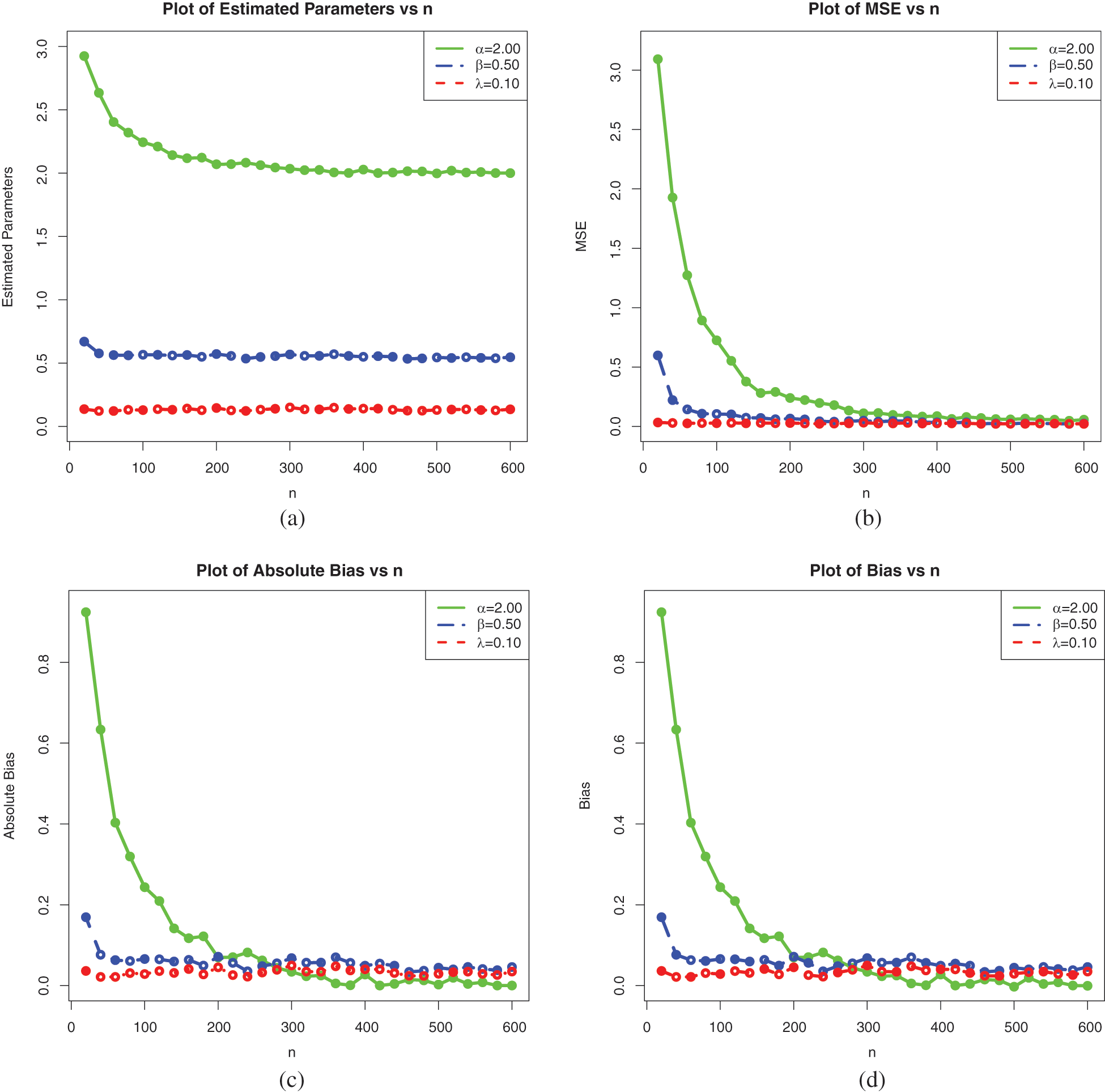
Figure 8: Plots of the simulation results on the estimates of the parameters of the ELo distribution for Set 3: (a) Average MLEs, (b) MSEs, (c) Absolute biases and (d) Biases

These tables and figures reveal that MLEs perform well for estimating the parameters of the ELo distribution. Indeed, as sample size increases, both the bias and MSE are reduced. Therefore, the MLEs and their asymptotic properties can be used quite efficiently. It is worth noting that the MLEs for the parameters in Sets 2 and 3 have better behavior than those in Set 1, especially regarding the estimation of β, which is taken larger. Additional tests prove that, for the considered sets and all the parameters, the estimation becomes quite efficient for a greater value of n.

We complete the above analysis with a precise study of the mean absolute error (MAE) defined by

MAE(θ^)=∑i=1600|θi^−θ|600(56)

where θ∈{α,β,λ}, and the index i refers to the ith sample for the given sample size, for Sets 1, 2, and 3.

The results are presented in Table 4.

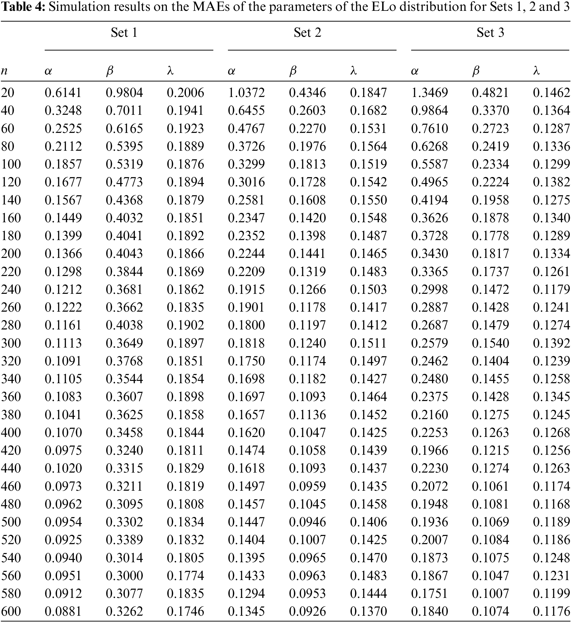
Table 4 is supported graphically by Fig. 9.

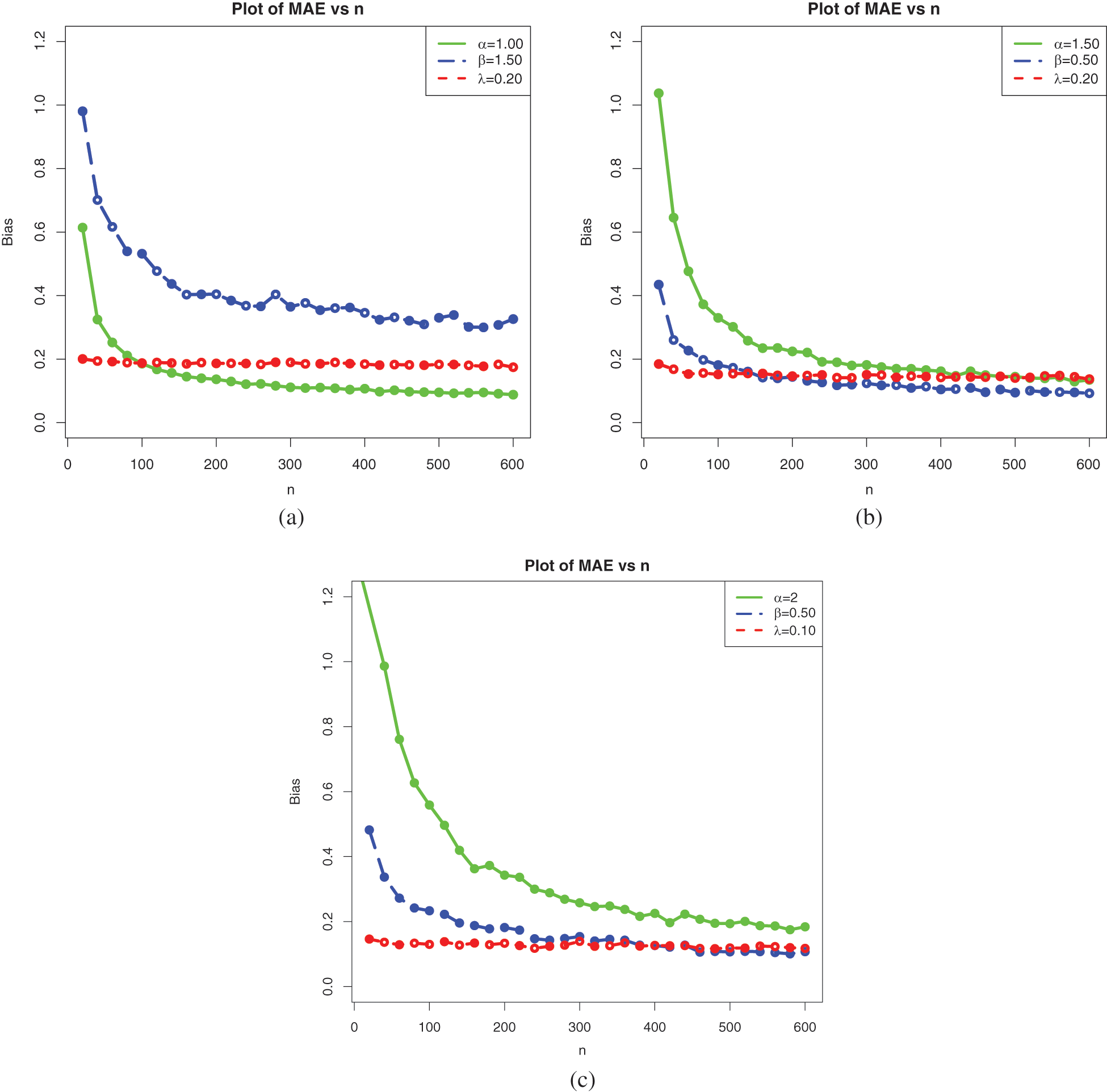
Figure 9: Plots of the simulation results on the MAEs for Sets 1, 2, and 3: (a) Set 1, (b) Set 2, and (c) Set 3

As expected, the results show a nice performance of the considered estimates based on the MAE measure.

In the rest of the study, they are used for data fitting purposes and actuarial measure estimation.

5  Applications

In this section, various applications of the ELo distribution are given based on two insurance claim data sets.

5.1 Data Fitting

This part is devoted to the efficiency of the ELo distribution in the fit of data sets with a heavy tail. To this end, we consider two Kenya car insurance claim data sets from the following link (https://data.world/datasets/insurance/). The first Data Set contains the number of claims from 2012 to 2015, named Data Set 1, while the second Data Set contains the third party theft and fire number of claims from 2012 to 2015, named Data Set 2. The boxplots of these data sets are presented in Fig. 10.

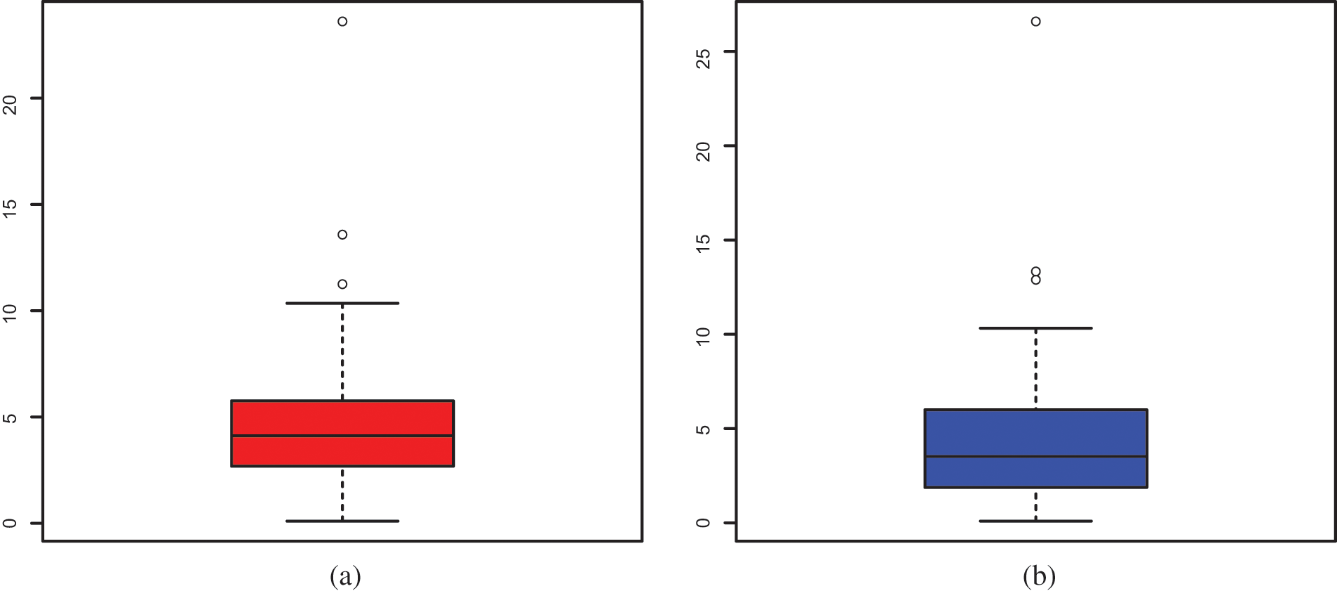
Figure 10: Box plot of (a) Data Set 1 and (b) Data Set 2

From Fig. 10, we observe that the distribution of the data for the two data sets is far too extreme to be in adequation with a normal distribution, with several extreme values. Heavy-tailed distributions are ideal for capturing them in particular and revealing the information behind them.

In addition, with these data, we aim to compare the ELo distribution, with some well-established heavy-tailed distributions, namely the complimentary Dagum Poisson (CDP), Poisson Lomax (PLo), exponentiated Lomax (ExLo), Burr-XII (BX11), Fréchet (Fr), Dagum (Da), inverse Weibull (IW) and Lo distributions. The reader is referred to [52] for a detailed discussion of statistical size distributions used in economics and actuarial sciences. It is worth noting that more extended Lo distributions have been tested for the considered data, but due to unsatisfactory results, they are not presented in the study.

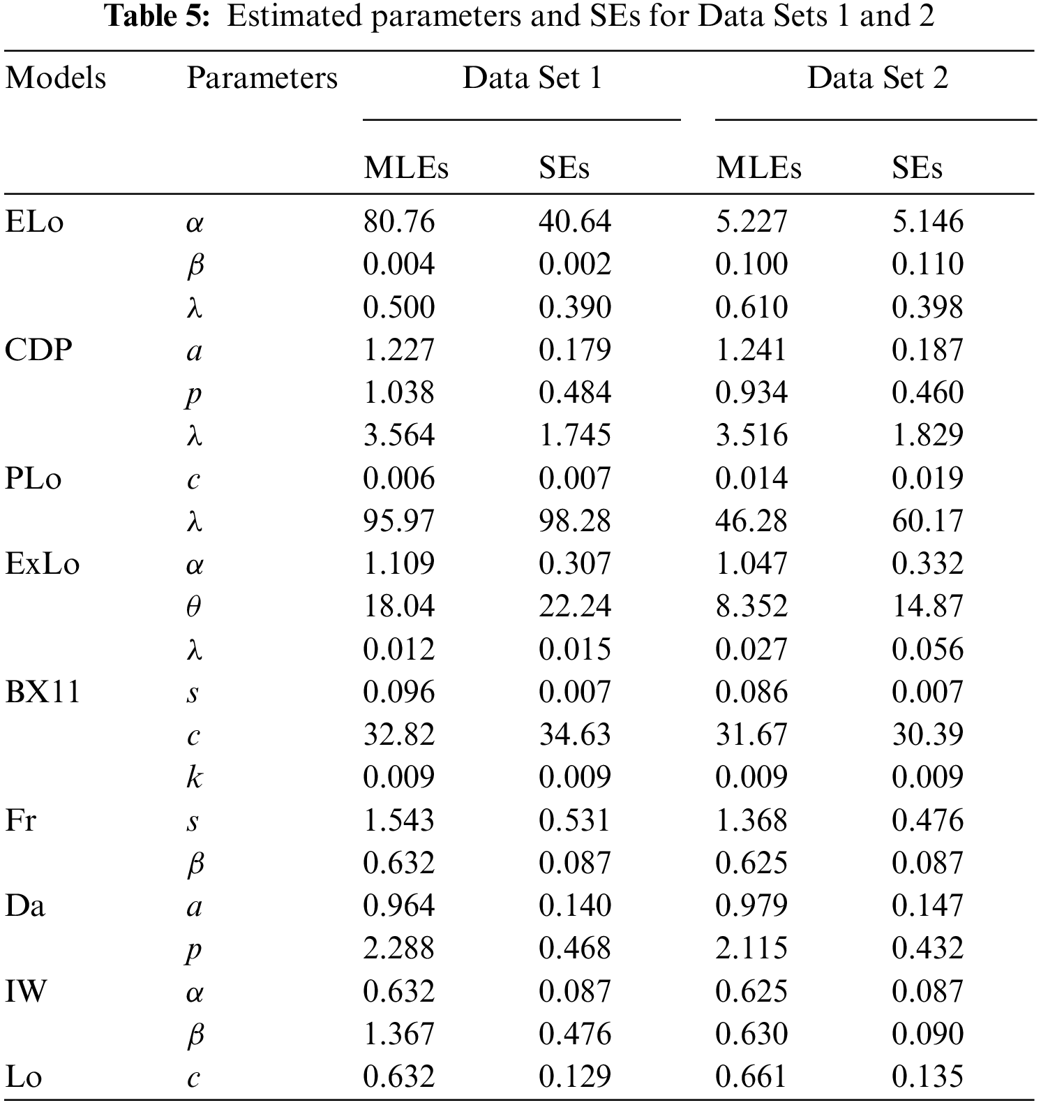
As sketched in the previous section, the AdequacyModel package is used in R-StatisticalComputing Environment to compute the MLEs and SEs of the distribution parameters. The log-likelihood function is evaluated at the MLEs (ℓ^). For model comparison, some well-known goodness-of-fit (GoF) statistics are considered. More precisely, the Akaike information criterion (AIC), Bayesian information criterion (BIC), Hannan-Quinn information criterion (HQIC), Anderson-Darling (A∗), Cramér–von Mises (W∗), and Kolmogrov-Smirnov (K-S), are used. The low values of GoFS and high K-S p-values indicate good fits.

MLEs and their respective SEs for the ELo, CDP, PLo, ExLo, BX11, Fr, Da, IW and Lo distributions which are calculated for the two data sets. They are displayed in Table 5. It is worth mentioning that the scale parameters of the CDP and Da distributions are considered as units.

The values of the GoFs are reported in Tables 6 and 7 for Data Sets 1 and 2, respectively.

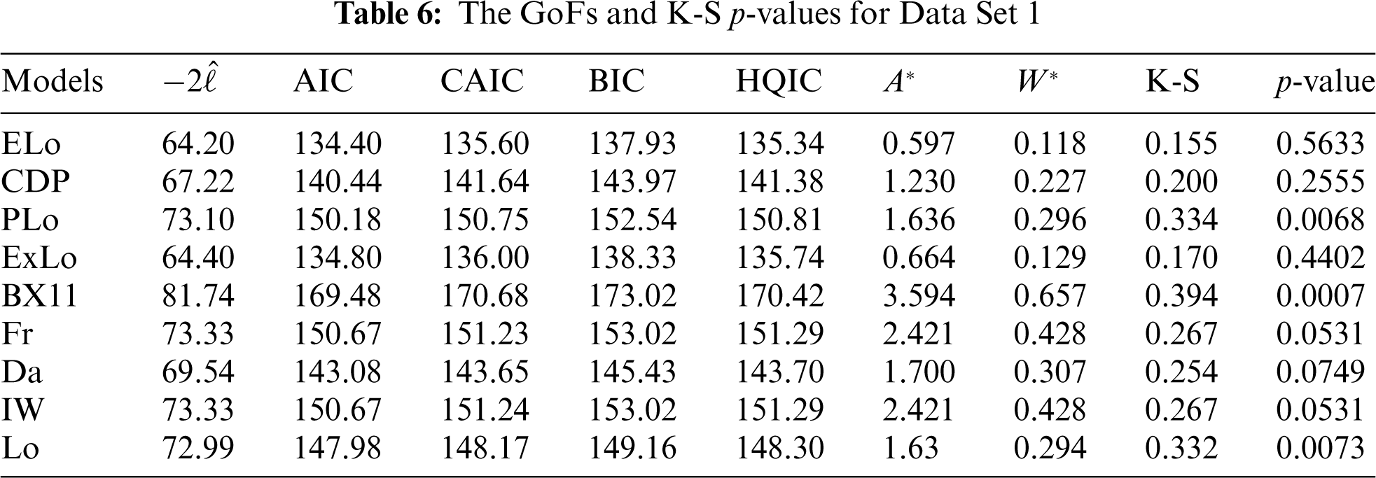
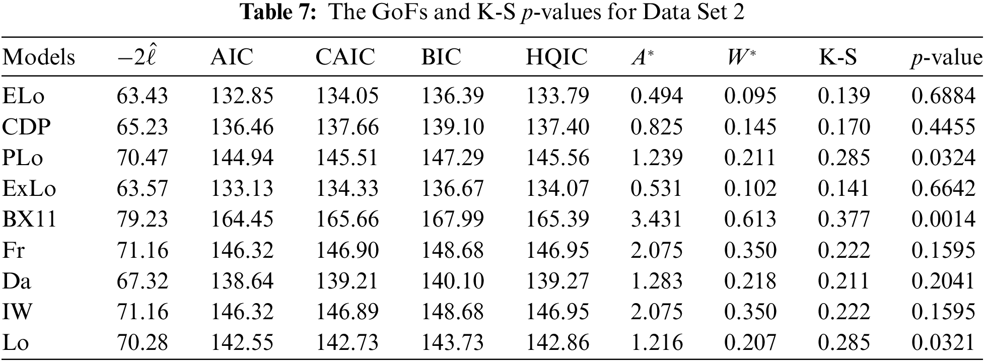
According to Tables 6 and 7, the proposed ELo distribution fits both data sets better than all other competitor distributions because it has the lowest AIC, BIC, HQIC, A∗, W∗, and K-S values. The K-S p-value satisfied p-value >0.05. We complete these numerical observations with graphical evidence. In Figs. 11 and 12 plot the estimated pdfs and cdfs of the ELo distribution, i.e., f^ELo(x), and F^ELo(x).

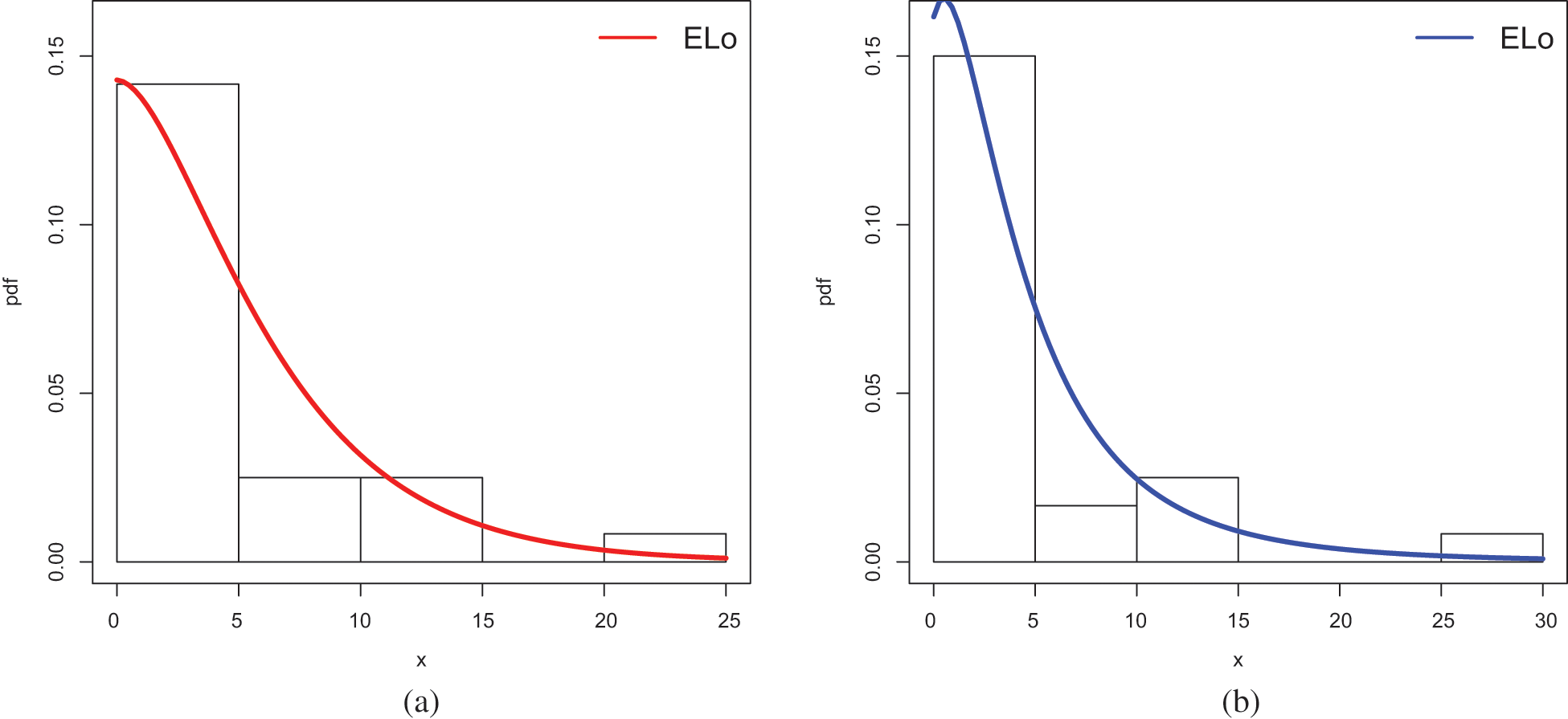
Figure 11: Plots of the estimated pdfs of the ELo distribution for (a) Data Set 1 and (b) Data Set 2

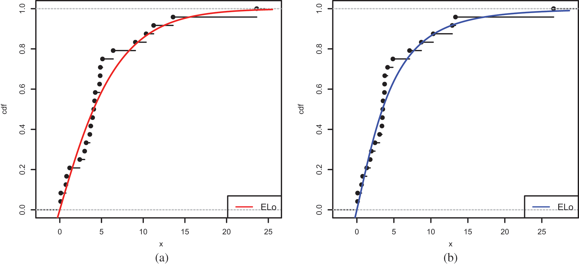
Figure 12: Plots of the estimated cdfs of the ELo distribution for (a) Data Set 1 and (b) Data Set 2

The estimated functions of the ELo distribution have good fits, which supports the numerical results of the study.

This is also confirmed by a quantile estimation analysis; we plot the quantile-quantile (Q-Q) plots of both data sets in Fig. 13.

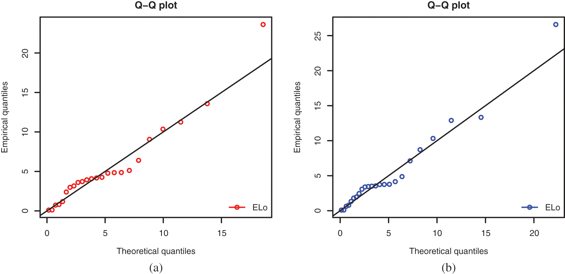
Figure 13: Q-Q-plots for the ELo distribution for (a) Data Set 1 and (b) Data Set 2

It is clear that the scatter plots are well adjusted by the respective Q-Q lines, proving the fit hability of the ELo distribution.

5.2 Numerical Illustration of VaR and ES

Here, since Data Sets 1 and 2 are well fitted by the ELo distribution, we provide estimates of the unknown associated risk measures VaR and ES. More precisely, a comparative study of VaR and ES for the ELo distribution with other heavy-tailed distributions: the ExLo, Lo and Da distributions, is performed by taking the MLEs of the parameters. It is worth emphasizing that a distribution with higher values of the risk measures is said to have a heavier tail.

Tables 8 and 9 provide the estimates of VaRs and ESs for the considered distributions based on Data Sets 1 and 2.

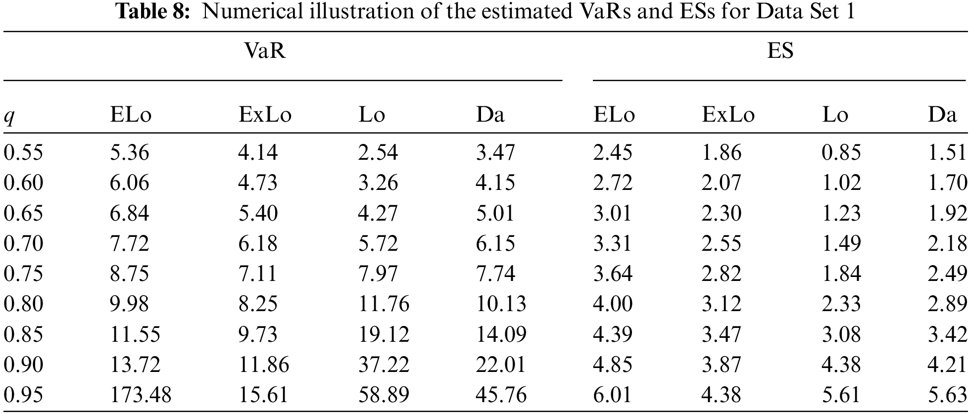
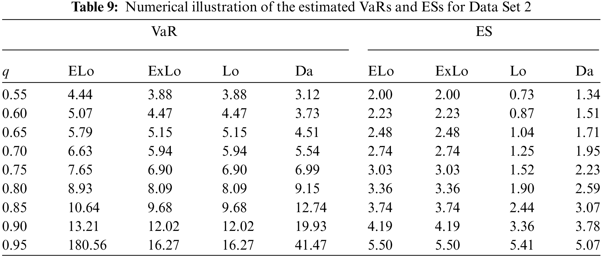
From these tables, it can be concluded that the ELo distribution has higher values of both the risk measures as compared to its counterparts, the ExLo, Lo, and Da distributions. The graphical demonstration of this statement can be seen in Figs. 14 and 15, where it is also revealed that the ELo distribution has a heavier tail than the ExLo, Lo, and Da distributions. The reader is referred to [53] for a detailed discussion of VaR and ES and their computation by using an R package.

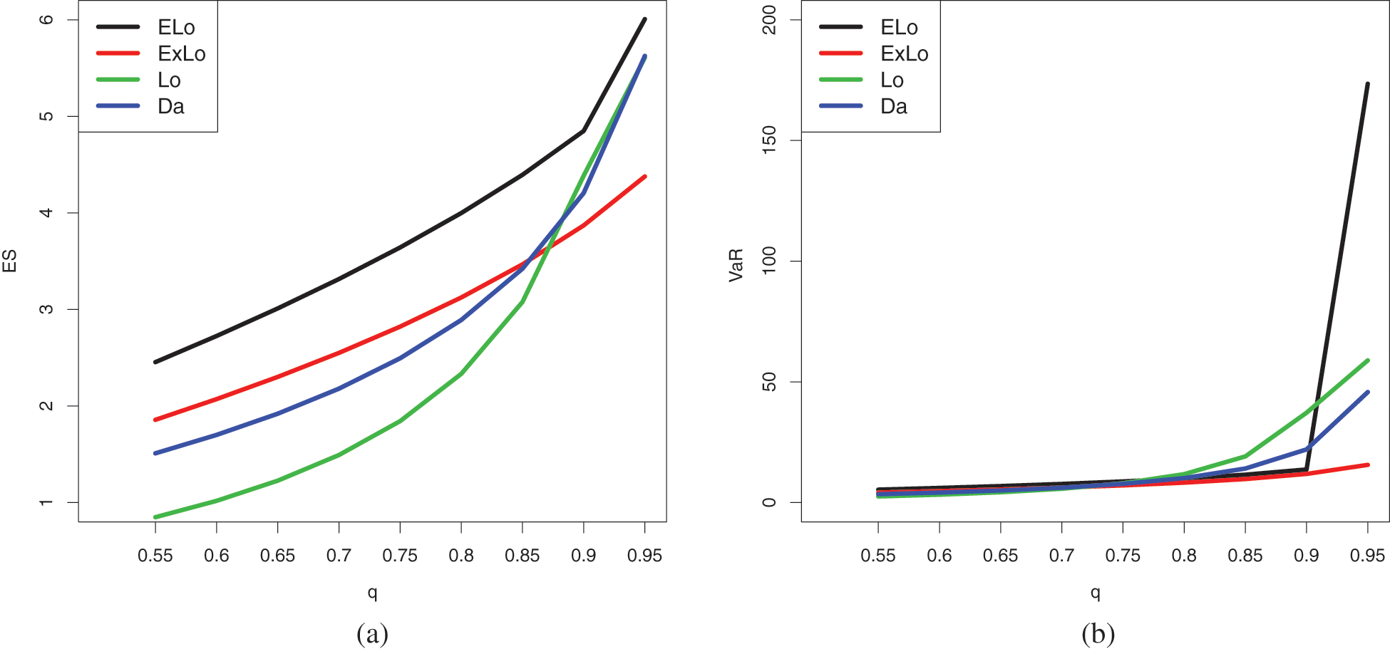
Figure 14: Plots of the estimated (a) ES and (b) VaR of the conidered distributions for Data Set 1

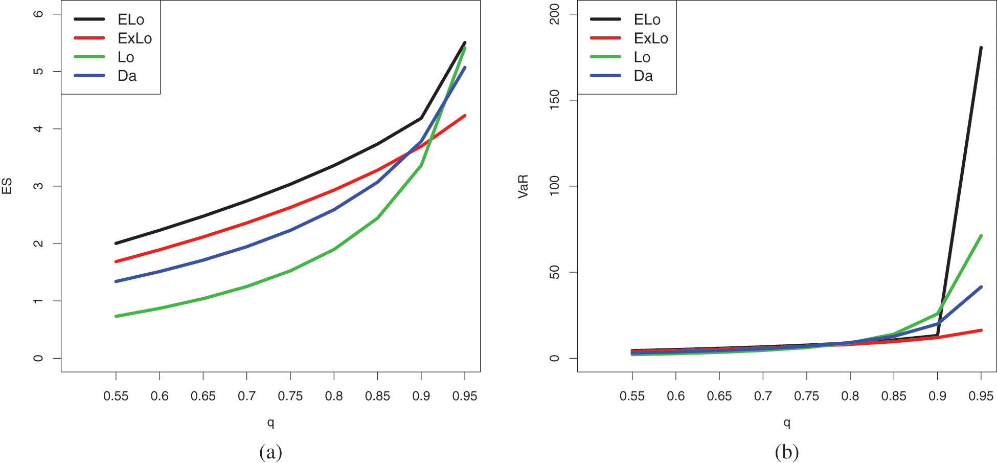
Figure 15: Plots of the estimated (a) ES and (b) VaR of the conidered distributions for Data Set 2

6  Conclusion

In this paper, we introduced a new three-parameter heavy-tailed extension of the Lomax distribution. It can be derived from a simple transformation of an existing unit distribution: the log-weighted power distribution. Some mathematical and statistical properties are derived, including the shapes of related probability and hazard rate functions; stochastic comparisons; manageable expansions for various moments; and quantile properties. Unknown parameters are estimated using the maximum likelihood method. A complete simulation study validates the accuracy of the obtained estimates. Two applications, each with its own plots, are provided to demonstrate the importance of the extended Lomax distribution. In particular, we show that it outperforms eight comparable distributions in the literature. Because of the heavy-tailed nature of the considered distribution, actuarial measures of importance are emphasized. Based on these actuarial measures, we show that it yields superior conclusions from fair competitor distributions.

We believe that the proposed methodology can be used quite efficiently to analyze data presenting a heavy-tail, especially for those having acceptable results with the Lomax distribution; the extended Lomax distribution will probably do the analysis in a more precise manner. Possible further work includes bivariatization and discretization of the extended Lomax distribution for different modeling objectives.

Acknowledgement: The authors would like to thank the three reviewers for their constructive comments on the paper.

Funding Statement: This project was funded by the Deanship Scientific Research (DSR), King Abdulaziz University, Jeddah, under the Grant No. KEP-PhD:21-130-1443. The authors acknowledge with thanks DSR for technical and financial support.

Availability of Data and Materials: The data used in this article are freely available in the mentioned references.

Conflicts of Interest: The authors declare that they have no conflicts of interest to report regarding the present study.

References

1. Balkema, A. A., de Haan, L. (1974). Residual life time at great age. The Annals of Probability, 2(5), 792–804. https://doi.org/10.1214/aop/1176996548 [Google Scholar] [CrossRef]
2. Bryson, M. C. (1974). Heavy-tailed distributions: Properties and tests. Technometrics, 16(1), 61–68. https://doi.org/10.1080/00401706.1974.10489150 [Google Scholar] [CrossRef]
3. Ahsanullah, M. (1991). Record values of Lomax distribution. Statistica Neerlandica, 41(1), 21–29. https://doi.org/10.1111/j.1467-9574.1991.tb01290.x [Google Scholar] [CrossRef]
4. Balakrishnan, N., Ahsanullah, M. (1994). Relations for single and product moments of record values from Lomax distribution. Sankhya B, 56(2), 140–146. [Google Scholar]
5. Childs, A., Balakrishnan, N., Moshref, M. (2001). Order statistics from non-identical right truncated Lomax random variables with applications. Statistical Papers, 42(2), 187–206. https://doi.org/10.1007/s003620100050 [Google Scholar] [CrossRef]
6. Arnold, B. C., Castillo, E., Sarabia, J. M. (1998). Bayesian analysis for classical distributions using conditionally specified priors. Sankhya B, 60(2), 228–245. [Google Scholar]
7. Howlader, H. A., Hossain, A. M. (2002). Bayesian survival estimation of Pareto distribution of the second kind based on failure censored data. Computational Statistics & Data Analysis, 38(3), 301–314. https://doi.org/10.1016/S0167-9473(01)00039-1 [Google Scholar] [CrossRef]
8. Cramer, E., Schmied, A. B. (2001). Progressively type-II censored competing risks data from Lomax distributions. Computational Statistics & Data Analysis, 55(3), 1285–1303. https://doi.org/10.1016/j.csda.2010.09.017 [Google Scholar] [CrossRef]
9. Al-Zahrani, B., Al-Sobhi, M. (2013). On parameters estimation of Lomax distribution under general progressive censoring. Journal of Quality and Reliability Engineering, 2013, 7, 431541. https://doi.org/10.1155/2013/431541 [Google Scholar] [CrossRef]
10. Johnson, N., Kotz, S., Balakrishnan, N. (1994). Continuous univariate distribution, 2nd edition, vol. 1. New York: Wiley. [Google Scholar]
11. Ghitany, M. E., Al-Awadhi, F. A., Alkhalfan, L. A. (2007). Marshall-Olkin extended Lomax distribution and its application to censored data. Communications in Statistics−Theory and Methods, 36(10), 1855–1866. https://doi.org/10.1080/03610920601126571 [Google Scholar] [CrossRef]
12. Al-Zahrani, B., Sagor, H. (2015). Statistical analysis of the Lomax-logarithmic distribution. Journal of Statistical Computation and Simulation, 85(9), 1883–1901. https://doi.org/10.1080/00949655.2014.907800 [Google Scholar] [CrossRef]
13. Abdul-Moniem, I. B. (2012). Recurrence relations for moments of lower generalized order statistics from exponentiated Lomax distribution and its characterization. Journal of Mathematical and Computational Science, 2, 999–1011. [Google Scholar]
14. Rajab, M., Aleem, M., Nawaz, T., Daniyal, M. (2013). On five parameter beta Lomax distribution. Journal of Statistics, 20(1), 102–118. [Google Scholar]
15. Al-Jarallah, R. A., Ghitany, M. E., Gupta, R. C. (2014). A proportional hazard Marshall-Olkin extended family of distributions and its application to Gompertz distribution. Communications in Statistics-Theory and Methods, 43(20), 4428–4443. https://doi.org/10.1080/03610926.2012.715226 [Google Scholar] [CrossRef]
16. El-Bassiouny, A. H., Abdo, N. F., Shahen, H. S. (2015). Exponential Lomax distribution. International Journal of Computer Applications, 121(13), 24–29. https://doi.org/10.5120/21602-4713 [Google Scholar] [CrossRef]
17. Cordeiro, G. M., Ortega, E. M., Popovic, B. V. (2015). The gamma-Lomax distribution. Journal of Statistical Computation and Simulation, 85(2), 305–319. https://doi.org/10.1080/00949655.2013.822869 [Google Scholar] [CrossRef]
18. Tahir, M. H., Cordeiro, G. M., Mansoor, M., Zubair, M. (2015). The Weibull-Lomax distribution: Properties and applications. Hacettepe Journal of Mathematics and Statistics, 44(2), 455–474. [Google Scholar]
19. Mead, M. E. (2016). On five-parameter Lomax distribution: Properties and applications. Pakistan Journal of Statistics and Operation Research, 12(1), 185–200. https://doi.org/10.18187/pjsor.v11i4.1163 [Google Scholar] [CrossRef]
20. Rady, E. H. A., Hassanein, W. A., Elhaddad, T. A. (2016). The power Lomax distribution with an application to bladder cancer data. SpringerPlus, 5(1), 1–22. https://doi.org/10.1186/s40064-016-3464-y [Google Scholar] [PubMed] [CrossRef]
21. Hassan, A. S., Abd-Allah, M. (2018). Exponentiated Weibull-Lomax distribution: Properties and estimation. Journal of Data Science, 16(2), 277–298. [Google Scholar]
22. Elbiely, M. M., Yousof, H. M. (2019). A new extension of the Lomax distribution and its applications. Journal of Statistics and Applications, 2(1), 18–34. [Google Scholar]
23. Nagarjuna, B. V., Vardhan, R. V. (2020). Marshall-Olkin exponential Lomax distribution: Properties and its application. Stochastic Modelling and Applications, 24, 161–177. [Google Scholar]
24. Al-Marzouki, S., Jamal, F., Chesneau, C., Elgarhy, M. (2020). Type II Topp-Leone power Lomax distribution with applications. Mathematics, 8(1), 1–26. [Google Scholar]
25. Mathew, J., Chesneau, C. (2020). Some new contributions on the Marshall-Olkin length biased Lomax distribution: Theory, modelling and data analysis. Mathematical and Computational Applications, 25(79), 1–21. https://doi.org/10.3390/mca25040079 [Google Scholar] [CrossRef]
26. Nagarjuna, B. V., Vardhan, R. V., Chesneau, C. (2021a). Kumaraswamy generalized power Lomax distribution and its applications. Stats, 4(1), 28–45. https://doi.org/10.3390/stats4010003 [Google Scholar] [CrossRef]
27. Ali, M. M., Yousof, H. M., Ibrahim, M. (2021). A new Lomax type distribution: Properties, copulas, applications, Bayesian and non-Bayesian estimation methods. International Journal of Statistical Sciences, 21(2), 61–104. [Google Scholar]
28. Nagarjuna, B. V., Vardhan, R. V., Chesneau, C. (2021b). On the accuracy of the sine power Lomax model for data fitting. Modelling, 2(1), 78–104. https://doi.org/10.3390/modelling2010005 [Google Scholar] [CrossRef]
29. Nagarjuna, V. B. V., Vardhan, R. V., Chesneau, C. (2022). Nadarajah-Haghighi Lomax distribution and its applications. Mathematical and Computational Applications, 27(30), 1–13. https://doi.org/10.3390/mca27020030 [Google Scholar] [CrossRef]
30. Almarashi, A. M. (2021). A new modified inverse Lomax distribution: Properties, estimation and applications to engineering and medical data. Computer Modeling in Engineering & Sciences, 127(2), 621–643. https://doi.org/10.32604/cmes.2021.014407 [Google Scholar] [CrossRef]
31. Abiodun, A. A., Ishaq, A. I. (2022). On Maxwell-Lomax distribution: Properties and applications. Arab Journal of Basic and Applied Sciences, 29(1), 221–232. https://doi.org/10.1080/25765299.2022.2093033 [Google Scholar] [CrossRef]
32. Khan, S., Hamedani, G. G., Reyad, H. M., Jamal, F., Shafiq, S. et al. (2022). The minimum Lindley Lomax distribution: Properties and applications. Mathematical and Computational Applications, 27(1), 16. https://doi.org/10.3390/mca27010016 [Google Scholar] [CrossRef]
33. Falgore, J. Y., Doguwa, S. I. (2022). On new Weibull inverse Lomax distribution with applications. Baghdad Science Journal, 19(3), 0528. [Google Scholar]
34. Aboraya, M., Ali, M. M., Yousof, H. M., Ibrahim, M. (2022). A novel Lomax extension with statistical properties, copulas, different estimation methods and applications. Bulletin of the Malaysian Mathematical Sciences Society, 45(Suppl 1), 85–120. [Google Scholar]
35. Lomax, K. S. (1954). Business failures; another example of the analysis of failure data. Journal of the American Statistical Association, 49, 847–852. https://doi.org/10.1080/01621459.1954.10501239 [Google Scholar] [CrossRef]
36. Chesneau, C. (2021). On a logarithmic weighted power distribution: Theory, modelling and applications. Journal of Mathematical Sciences: Advances and Applications, 67(1), 1–59. [Google Scholar]
37. Gómez-Déniz, E., Sordo, M. A., Calderín-Ojeda, E. (2014). The logLindley distribution as an alternative to the beta regression model with applications in insurance. Insurance: Mathematics and Economics, 54, 49–57. [Google Scholar]
38. Shaked, M., Shanthikumar, J. G. (1994). Stochastic orders and their applications. Boston: Academic Press [Google Scholar]
39. Bawa, V. S. (1975). Optimal rules for ordering uncertain prospects. Journal of Financial Economics, 2(1), 95–121. https://doi.org/10.1016/0304-405X(75)90025-2 [Google Scholar] [CrossRef]
40. Müller, A., Stoyan, D. (2002). Comparison methods for stochastic models and risks. Chichester: John Wiley & Sons. [Google Scholar]
41. Chamberlain, G. (1987). Asymptotic efficiency in estimation with conditional moment restrictions. Journal of Econometrics, 34(3), 305–334. https://doi.org/10.1016/0304-4076(87)90015-7 [Google Scholar] [CrossRef]
42. Kim, J. H. T. (2010). Conditional tail moments of the exponential family and its related distributions. North American Actuarial Journal, 14, 198–216. https://doi.org/10.1080/10920277.2010.10597585 [Google Scholar] [CrossRef]
43. Oakes, D., Desu, M. M. (1990). A note on residual life. Biometrica, 77, 409–410. https://doi.org/10.1093/biomet/77.2.409 [Google Scholar] [CrossRef]
44. Dress, H., Reiss, R. D. (1996). Residual life functionals at greate age. Communications in Statistics-Theory and Methods, 25(4), 823–835. https://doi.org/10.1080/03610929608831734 [Google Scholar] [CrossRef]
45. Ebrahimi, N. (1998). Estimating the finite population versions of mean residual life-time function and hazard function using Bayes method. Annals of the Institute of Statistical Mathematics, 50(1), 15–27. https://doi.org/10.1023/A:1003493112915 [Google Scholar] [CrossRef]
46. Galton, F. (1883). Enquiries into human faculty and its development. London: Macmillan & Company. [Google Scholar]
47. Moors, J. J. (1988). A quantile alternative for kurtosis. Statistician, 37, 25–32. https://doi.org/10.2307/2348376 [Google Scholar] [CrossRef]
48. Artzner, P., Delbaen, F., Eber, J. M., Heath, D. (1999). Coherent measures of risk. Mathematical Finance, 9(3), 203–228. https://doi.org/10.1111/1467-9965.00068 [Google Scholar] [CrossRef]
49. Gilchrist, W. (1997). Modelling with quantile distribution functions. Journal of Applied Statistics, 24(1), 113–122. https://doi.org/10.1080/02664769723927 [Google Scholar] [CrossRef]
50. Casella, G., Berger, R. L. (1990). Statistical inference. Bel Air, CA, USA: Brooks/Cole Publishing Company. [Google Scholar]
51. Algarni, A., Almarashi, A. M. (2022). A new Rayleigh distribution: Properties and estimation based on progressive type-II censored data with an application. Computer Modeling in Engineering & Sciences, 130(1), 379–396. https://doi.org/10.32604/cmes.2022.017714 [Google Scholar] [CrossRef]
52. Kleiber, C., Kotz, S. (2003). Statistical size distributions in economics and actuarial science. Wiley series in probability and statistics. Hoboken, New Jersey: Wiley Interscience, John Wiley and Sons Inc. [Google Scholar]
53. Chen, X., Chi, Y., Tan, K. S. (2016). The design of an optimal retrospective rating plan. ASTIN Bulletin, 46(1), 141–163. https://doi.org/10.1017/asb.2015.19 [Google Scholar] [CrossRef]
Cite This Article
Copyright © 2023 The Author(s). Published by Tech Science Press.
This work is licensed under a Creative Commons Attribution 4.0 International License , which permits unrestricted use, distribution, and reproduction in any medium, provided the original work is properly cited.
Downloads
Citation Tools