Floyd-Warshall Algorithm Based on Picture Fuzzy Information

1  Introduction

The Shortest Path Algorithm (SPA) is a family of graph algorithms designed to solve the Shortest Path Problem (SPP). In a graph, all nodes are joined by edges. If more than one route is available, the question arises as to which path should be chosen at the lowest cost or distance. The main goal of the SPA is to find the minimum cost path. There are two types of SPP, Single Source Shortest Path (SSSP) problem and All Pair Shortest Path (APSP) problem. The SSSP problem finds the shortest paths from a source vertex to all other vertices in the graph. APSP finds the shortest path between every pair of vertices in any graph. These algorithms are applicable in a variety of situations. A few of these include transportation networks, computer networks, Google maps, inventory systems, and labor locations, among many others. In all these real-world scenarios, we need to find the shortest path between any pair of points. How can the shortest path be found between any two nodes if the network situation is uncertain? The classic algorithm is appropriate when the network situation is certain and the weights are crisp. But, in reality, networks are not certain. Fuzzy set theory has been employed to deal with these uncertainties. This theory was presented by Zadeh in 1965 for making decisions under uncertain conditions [1]. In 1986, Atanassov introduced the extension of classical fuzzy sets and named it an Intuitionistic Fuzzy Set (IFS) [2]. In IFS, a set has two components: membership and non-membership. This new theory handled uncertainties more effectively and applied them to many fields. After a few years, it was experienced that in many cases, the neutral section needs to give more freedom to express the expert opinion. Consequently, in 2013 Cuong et al. introduced a general form of IFS called Picture Fuzzy Set (PFS) [3,4]. A real number can be generalized into a fuzzy number. Unlike trapezoidal intuitionistic fuzzy numbers discussed by Wan et al. [5], which only have two components, trapezoidal picture fuzzy numbers have three aspects for every input. There are membership and non-membership components in a trapezoidal intuitionistic fuzzy set. The hesitation component of this number can be obtained by deducting 1 from the total membership and non-membership values. Whereas, a trapezoidal intuitionistic fuzzy number is ineffective to illustrate the neutral part of a number, which is provided in a trapezoidal picture fuzzy number to give more flexibility to human opinion.

In 1980, Dubois et al. proposed the concept of fuzzy shortest path (FSP) [6]. They used the ranking index approach to find the shortest route. In 1994, Okada et al. [7] introduced an algorithm based on the Dijkstra algorithm in which they used fuzzy order to compare the lengths of the two routes for finding the FSP. In 2009, Mahdavi et al. [8] proposed a dynamic programming (DP) approach for FSPP, taking into account the length of the triangle and trapezoidal arc. In 2012, Dou et al. [9] offered a model for finding FSP using MCDM based on its earlier approach, i.e., measuring ambiguous similarities. So, there are various methods to find the SPP, some of which are discussed in [10,11]. The Floyd-Warshall algorithm uses the dynamic programming approach to find APSP, where the edge weight is given as a crisp number. Due to its structural similarities with matrix multiplication, it is an attractive choice for each pair of short paths in high-performance systems. This algorithm estimates the shortest path between the two vertices at each stage until the minimum value is achieved. Suppose G is a graph with V set of vertices, each numbered from 1 to N. To find the shortest path, there is the shortest path function (i, j, k), which returns the shortest path from i to j using k as an intermediate point. Garg et al. [12] suggested that the Floyd-Warshall algorithm can compete with Dijkstra’s algorithm for sparse graphs. If you have N nodes, then there are N−1 directed edges that can lead from it. Therefore, the maximum number of edges is N∗(N−1), and every possible edge is checked. It does this by incrementally improving the estimate of the shortest path between two vertices until the optimal path is obtained. Shukla [13] used graded mean integration representation of fuzzy numbers to upgrade the classical Floyd-Warshall algorithm. Aziz et al. [14] used the concept of Fuzzy and Floyd-Warshal algorithms to determine the shortest exit route for people living in catastrophically exposed areas. Shafahi et al. [15] proposed a new fuzzy comparing index for improving the fuzzy comparison method developed by Dubois and Prade to estimate and compare the distance between the assigned and observed link volumes. Broumi et al. [16] compared the shortest path problem with various existing algorithms. Akram et al. [17] extended the traditional Dijkstra algorithm to find out the minimal cost path using Picture fuzzy sets. Some other interesting approaches can be seen in [18–20]. Thao [21] presented similarity measures of Picture fuzzy sets caused by entropy and gave useful results. Mahmood et al. [22] explored the cross-entropy of the picture hesitant fuzzy set by distinguishing the cross-entropy of the picture fuzzy set and hesitant fuzzy set. Ganie et al. [23] proposed two correlation coefficients of PFS along with some of their properties. Nirmani et al. [24] developed a Google map and a camera-based fuzzy adaptive networked traffic light controlling model to minimize traffic in big cities, using a distributed system to scan the traffic lights. The author makes decisions based on real-time traffic situations. After these decisions, they monitored the traffic lights. They also proposed the optimized route to the drivers as an extra facility. Yue [25] proposed a novel bilateral matching decision-making for knowledge innovation management which reflects the matching willingness of the agents. Jiang et al. [26] proposed a new Picture fuzzy MABAC method for multiple attribute group decision-making. He applied this method in the manufacturing industry and shows that how it helps purchasers in choosing an optimal supplier. Habib et al. [27] used Pythagorean MCDM methods to determine childhood cancer. The proposed method helps to early diagnose childhood cancer. Akram et al. [28] and Habib et al. [29] proposed trapezoidal and LR-type Pythagorean fuzzy numbers and applied them to different optimization techniques. Zhang et al. [30] proposed novel distance measures of hesitant fuzzy sets. These formulas are based on probability density functions. The authors showed the applicability of the proposed measures in the traffic control system. Zhang et al. [31] introduced a new concept of neutrosophic decision-making in genetic algorithms and discussed its applicability in the cubic assignment problem. Yi et al. [32] presented an algorithm for path planning depending on the path conditions. This algorithm is applied and tested on the robot soccer, which plans a path after observing obstacles. After recognizing the environment, robot soccer determines the shortest path in the defined time frame.

The investigation presented in this article is motivated by the following targets:

1.    Shortest path problems, in literature, are classified as single-source shortest path problems and do not cover all pair shortest path problems.

2.    Real-time scenarios may involve ambiguity; therefore in typical situations, a crisp approach for APSP may not be appropriate.

3.    The IFS, on the other hand, deals with the membership and non-membership components of a set with the condition that their sum should not be greater than one, which leads to numerous problems in decision-making. The picture fuzzy set, which also includes the neural component of the set, is a generalization of IFSs. As a result, we have more degrees of freedom to make better decisions.

4.    The Floyd-Warshall algorithm has numerous real-time applications. In computer networks, for instance, calculating APSP from any source to any destination is necessary.

5.    Each edge may hold weights of various criteria; however, in most of the research studies, only one criterion is taken into consideration when assigning the weight of each edge.

Our contribution to this work is demonstrated below concerning these issues:

1.    We introduce a new variant of classical Floyd’s algorithm using trapezoidal picture fuzzy numbers. This algorithm computes the smallest weights of all possible routes for each pair of points. This algorithm is more effective in finding the shortest path.

2.    We design the algorithm and determine its time complexity to demonstrate the complete functioning of the picture fuzzy Floyd-Warshall (PF Floyd-Warshall).

3.    We contrast our approach with already used techniques to demonstrate how the suggested method is an improved version of the current ones.

4.    The suggested algorithm can select the optimum route using up to n criteria weights for each edge.

The rest of the paper is organized in the following way: Section 2 presents the concepts related to picture fuzzy sets. Section 3 discusses the complete working of the picture fuzzy Floyd-Warshall algorithm. Section 4 describes the implementation of the picture fuzzy Floyd-Warshall algorithm in networks. Section 5 gives a comparative analysis of PF Floyd-Warshall with the fuzzy Floyd-Warshall algorithm. Section 6 concludes this paper and displays feasible future directions.

2  Preliminaries

In this section, we recall some basic notions related to PFSs and PFNs.

Definition 2.1. [4] A Picture Fuzzy Set (PFS) S on universe U is defined as

S={(x,μS(x),νS(x),λS(x))|x∈U},(1)

where μS(x), νS(x), λS(x)∈ [0, 1] are called positive, neutral, and negative membership functions, respectively, of an element x in S such that

0≤μS(x)+νS(x)+λS(x)≤1,for every x∈U.

Moreover, πS(x)=1−μS(x)−νS(x)−λS(x) is called refusal membership degree of x to the set S.

Definition 2.2. [17] A PFN N in the set of real numbers R can be defined as N={(x,μN(x),νN(x),λN(x)):x∈R}, where

μN(x)={fNL(x),ifp1≤x≤q,αN,ifq≤x≤r,fNR(x),ifr≤x≤s1,0,otherwise.(2)

νN(x)={gNL(x),ifp2≤x≤q,βN,ifq≤x≤r,gNR(x),ifr≤x≤s2,0,otherwise.(3)

λN(x)={hNL(x),ifp3≤x≤q,γN,ifq≤x≤r,hNR(x),ifr≤x≤s3,0,otherwise.(4)

where fNL(x)=x−p1q−p1αN, fNR(x)=x−p1q−p1αN, gNL(x)=q−x+βN(x−p2)q−p2αN, gNR(x)=x−r+βN(s2−x)s2−r, hNL(x)=q−x+γN(x−p3)q−p3αN, hNR(x)=x−r+γN(s3−x)s3−r.

The TPFN is represented as

N=(([p1,q,r,s1];αN),([p2,q,r,s2];βN),([p3,q,r,s3];γN)).(5)

Example 2.1. Fig. 1 shows the plot for TPFN.

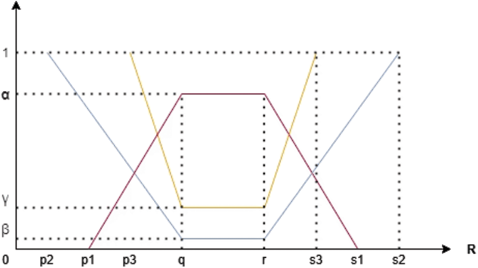
Figure 1: TPFN

Remark 2.1. If [p1,q,r,s1]=[p2,q,r,s2]=[p3,q,r,s3], then N can be characterized as

N=([p,r,q,s];αN,βN,γN).(6)

2.1 Arithmetic Operations on PFS

Some basic operations of PFS proposed by Akram et al. [17] is described below:

Let N1=([a1,b1,c1,d1];αN1,βN1,γN1) and N2=([a2,b2,c2,d2];αN2,βN2,γN2) be two TPFNs, then

1.    Addition:

N1+N2=([a1+a2,b1+b2,c1+c2,d1+d2].αN1+αN2−αN1αN2,βN1βN2,γN1γN2).(7)

2.    Multiplication:

N1.N2=([a1a2,b1b2,c1c2,d1d2];αN1αN2,βN1+βN2−βN1βN2,γN1+γN2−γN1γN2).(8)

3.    Multiplication with a constant: If k be a constant value then

kN1=([ka1,kb1,kc1,kd1];1−(1−αN1)k,βN1k,γN1k).(9)

4.    Power and exponent [17]: If k be an exponent value then

N1k=([a1k,b1k,c1k,d1k];αN1k,1−(1−βN1)k,1−(1−γN1)k),k≥0.(10)

2.2 Expected Value of TPFN

For a trapezoidal PFN N=([p,q,r,s];αN,βN,γN), the expected value is determined according to the formula suggested in [17] as follows:

IN=18[(p+q+r+s)(1+αN−βN−γN)].(11)

Definition 2.3. [17] Let N=([p,q,r,s];αN,βN,γN) be TPFN, then the score function S(N) of a PFN N can be calculated as follows:

§(N)=IN(αN−βN−γN),(12)

where IN is the expected value of N and S(n) lies between [−1,1].

Definition 2.4. [17] Let N=([p,q,r,s];αN,βN,γN) be TPFN, then the accuracy function H(N) of a PFN N can be calculated as follows:

H(n)=IN(αN+βN+γN),(13)

where IN is the expected value of N and H(n) lies between [0, 1].

Certain new methods have been discussed in [33,34].

Definition 2.5. [33] A linguistic variable is a variable, whose values are words or sentences in a natural or artificial language. These linguistic terms are very close to human understanding, so instead of remembering picture fuzzy numbers, the user can use these terms. These variables also hide the complexity of the system and make it more understandable. Picture fuzzy numbers are also denoted by some linguistic terms. For example, very low is a linguistic variable and its corresponding TPFN is ([1, 2, 3, 5]; 0.6, 0.1, 0.2) (see Eq. (6)). The linguistic variables and their picture fuzzy numbers are pre-defined.

2.3 Classical Floyd-Warshall Algorithm

The classical Floyd-Warshall algorithm described in [13] is used for finding APSP. Lets consider three weighted nodes x, y, and k to find shortest path from x to y via k node using following equation:

axk+aky<axy.(14)

k is the pivotal point and its value lies between 1 to n.

The step-by-step execution of this algorithm is given below:

Step 1: Initialize the graph using certain values defined by the user. Build a square matrix that consists of n rows and columns. Each entry is represented as Aij that shows the weight between i and j node. If there exists no edge between x and y, then it is represented by infinity. The working of this algorithm starts with two matrices, which are weight matrix A0 and sequence matrix B0. The diagonal values are 0 because we ignore self-loops. The other values are obtained from the weights mentioned on each edge in a graph.

                         1          2       ....    j         ....      nA0=12..x..n(0a12....axy....na210....a2y....a2n::::::ax1ax2....axy....axn::::::xn1xn2....xny....0)                                1     2      ....      j     ....  nand  B0=12..x..n(02....y....n10....y....n::::::12....y....n::::::12....y....0)

Step 2: Take k as a pivot row and k pivot column and for all x and y we perform triple operation on every axy in Ak−1. If axk+aky<axy condition meets for x, y and k then change Ak and Bk values using following rules:

•   Define Ak by replacing axy in Ak−1 with axk + aky,

•   Define Bk by replacing bxy in Sk−1 with k. If k=n then stop the loop otherwise repeat this step with the next value of k.

Step 3: After n steps, we get final matrices An, and Bn containing APSP. We read the final matrices using the following rules:

•   From An, axy shows the weights of short path between x, y vertices.

•   From Bn, get the intermediate node k=bxy that gives the route x → y →k.

Stop the iterations when bxk=k and bky=j and APSP has been determined.

3  Picture Fuzzy Floyd-Warshall Algorithm

In this section, we propose a new variant of the classical Floyd-Warshall algorithm. We apply PFN on Floyd-Warshall Algorithm to find APSP. Table 1 shows the description of the notions used in this article.

The step-by-step execution of the proposed algorithm is given below:

Step 1: Initially, label each edge with the appropriate PFN. These PFNs are acting as weights. If there is more than one criterion, the edge carries more than one PFN separated by commas. As we want to find the shortest path, therefore self-loops are avoided. The self-loops need to remove.

Step 2: Write initial matrix An, and sequence matrix Bn. These weights are calculated using Eqs. (11) and (12). These matrices are square matrices with n number of rows and columns. In this matrix, all diagonals are set to zero because self-loops are not allowed. If no direct path exists between any pair of nodes, set ∞ in its place; otherwise with the help of Eqs. (11) and (12) calculate the value of that cell. The sequence matrix shows the number of the intermediate node. The intermediate node k that gives a favorable value would be written in that cell in a sequence matrix.

Step 3: The next task is to find the shortest path between any pair of nodes. For this, use Eq. (14) to find the shortest path from x to y via k. In the single iteration, we may not get the shortest path for all pairs of nodes; therefore this step needs to repeat for all pairs in a graph. When k=n, terminate the loop and display the final weights and the sequence matrix. At this step, all intermediate nodes get discovered, and the obtained weight and sequence matrices are the final findings of this algorithm. If more than one criteria involve, then in all iterations, we compare each criterion with its previous state, if its value is in favor, we assign it a boolean label true otherwise false.

Step 4: Pick the value in the vector that has the most true values.

Fig. 2 shows the pictorial representation of the picture fuzzy Floyd-Warshall algorithm.

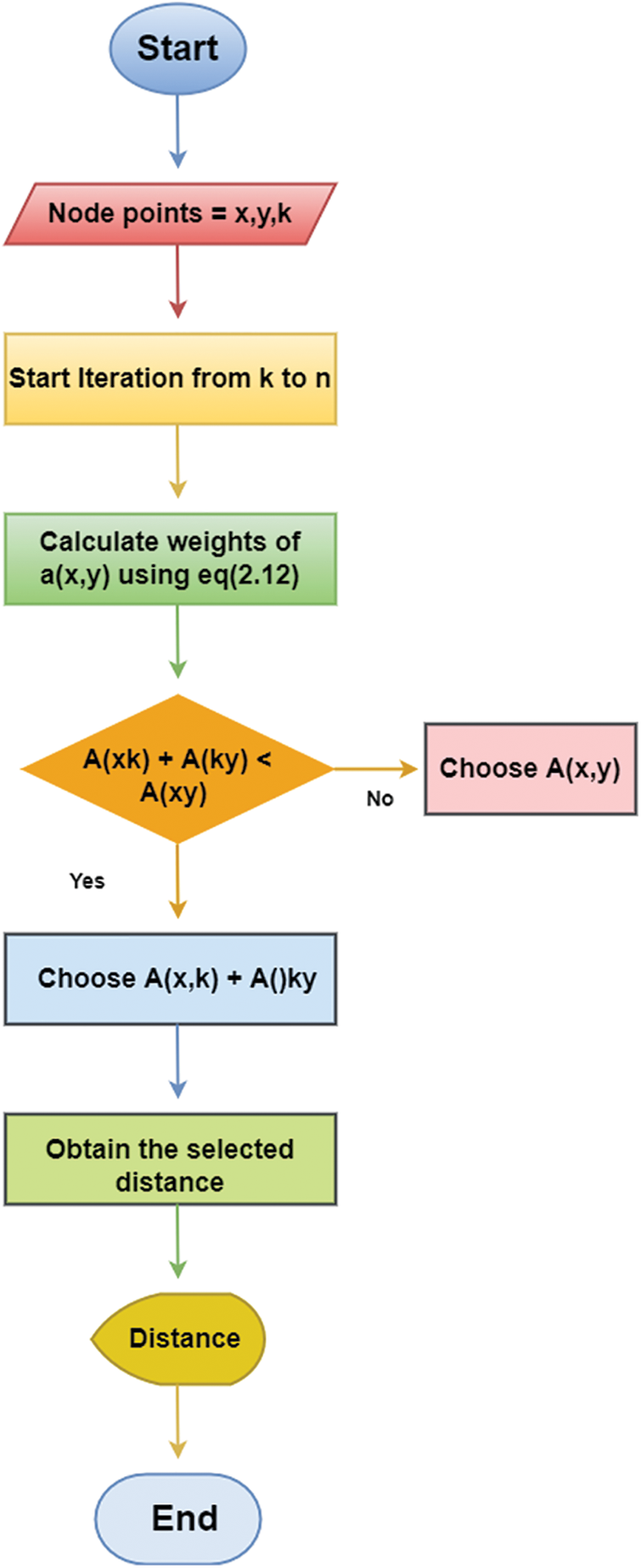
Figure 2: Flowchart of picture fuzzy Floyd-Warshall algorithm

3.1 Presentation and Complexity of the Algorithm

The following algorithm helps to understand the complete working of PF Floyd-Warshall algorithm:

:

Let us compute the time complexity of the above algorithm. Line 1 defines the function’s name and takes graph G as input. Here, G represents the layout of a network. In line 3, we take two integers x and y to locate cell values in a two-dimensional array and initialize them with 0. In line 4, a square matrix A of n×n dimensions are defined and initialized with ∞. Now use Eqs. (11) and (12) to calculate the distance between x and y. If there is no path between x and y then represent it with infinity. Lines 1–4 take constant time. In line 5, we define a loop that iterates for rows. There is n number of rows, therefore line 5 runs in O(n) times. Similarly, in line 6 a nested loop is defined for addressing the number of columns. It takes O(n2) running time. These loops help to locate the values of each cell in a matrix. The value of each cell is represented by pair of values (x,y) in matrix A. In lines 7–12, we see that if the value of x is not equal to the value of y, and there’s an edge between x and y, then calculate the distance value using Eqs. (11) and (12) otherwise write infinity. The diagonal values are 0 because self-loops are not allowed. Lines 7–12 run in O(n2) time. In line 13, we take another loop for finding the shortest path from x to y. Here k is considered as a breaking point. The value of k lies between 1 to n. Line 13 runs in O(n) times. Line 14 runs in O(n2) time. Line 15 takes O(n3) time. These loops iterate until the final shortest path is not found. Line 16 takes O(n3) time. Line 17 shows the final result, and it takes O(1) time. Therefore, the overall time complexity of the algorithm is O(n3).

3.2 Example

This section illustrates the working of our proposed algorithm. For this purpose, consider a transportation network shown in Fig. 3. The transition time on edges is represented as TPFN edge (3,5) is directed, so no traffic is allowed from node 5 to 3. All other edges allow two-way traffic. First of all, we calculate the distance value of each pair of edges using Eqs. (11) and (12) (see Table 6).

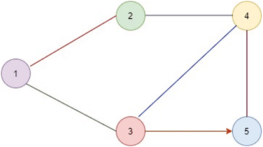
Figure 3: Transportation network model

For edge (1,2), the distance value is calculated as follows:

I1−2=18[(1+2+3+5)×(1+0.6−0.1−0.2)]=1.787,

S1−2=1.7875×(0.6−0.1−0.2)=0.53625.

In the same way, we compute the distance for other pairs. Table 2 shows the weights on each edge.

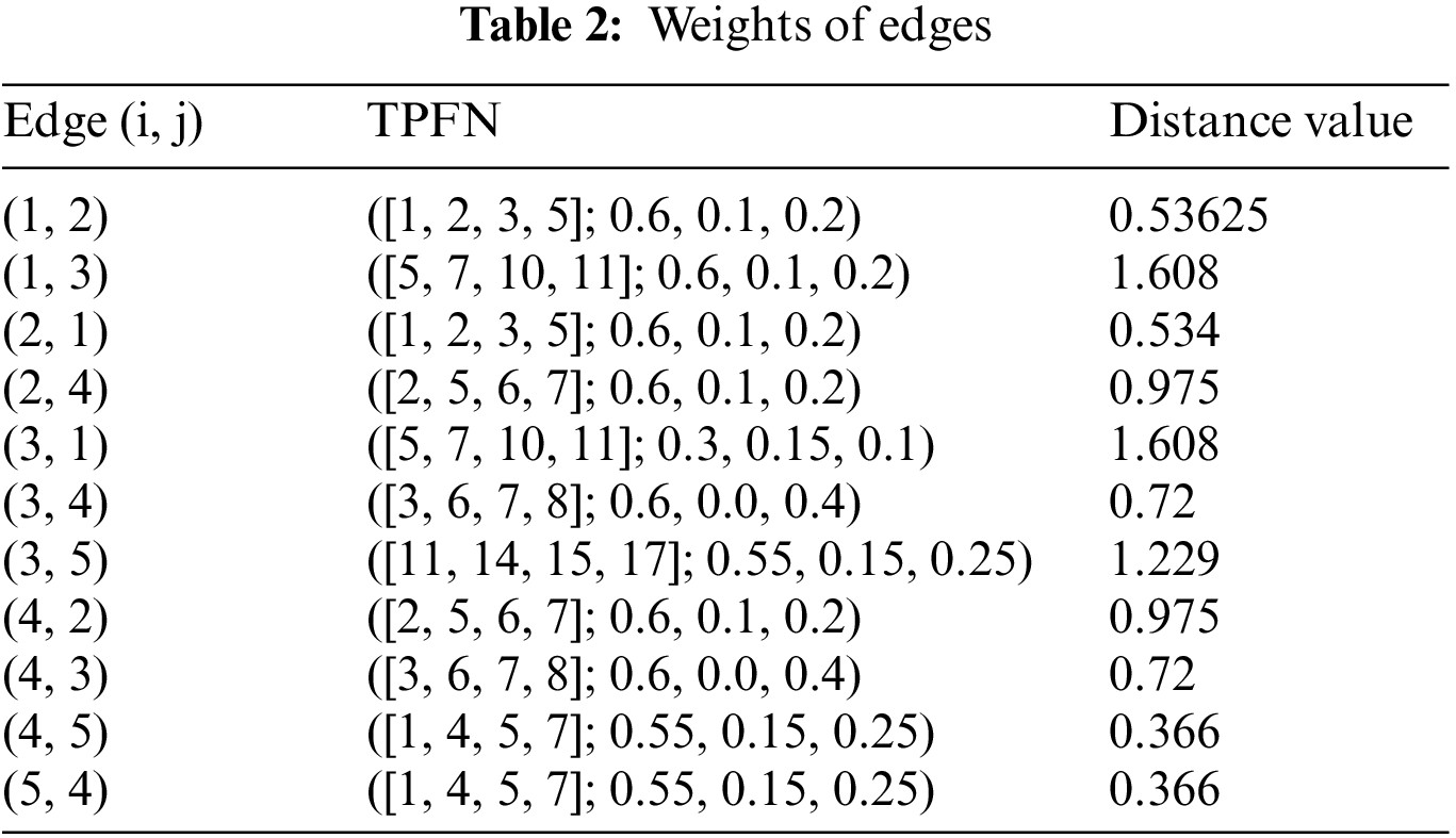
Iteration 0:

The matrices A0 and B0 give the initial values of the network, where all (x,y)th entries of A0 are canonical representations of weights of route from x to y. The matrix A0 and B0 are as follows:

                  01          02            03             04            05   A0=12345(00.5361.608∞∞0.5360∞0.975∞1.608∞00.721.2291∞0.9750.7200.366∞∞∞0.3660)              01   02   03  04  05,B0=12345(0234510345120451230512340)

All iterations of the picture fuzzy Floyd-Warshall algorithm are shown in Table 3.

The obtained results are the same as proposed in [13]. For instance, shortest route from node 1 to 5 is 1→2→4→5. Both algorithms highlighted the same paths for every set of vertices.

4  Application of Picture Fuzzy Floyd-Warshall Algorithm in Routing

The computer network is the interconnection of multiple communicating devices so that they can share their resources. To share their resources, we need routes. These routes can be wired or wireless. In computer networks, multiple routes can exist between any pair of nodes. Among these routes, we need to choose the best route for sending data. Different parameters help to determine the best route among all available routes. Examples of such parameters are length, bandwidth, load, hop count, cost, delay, maximum transmission unit, and reliability. Fig. 4 shows a hypothetical layout of a network, where all nodes can communicate with each other, but the question is which path is good for communication at any particular time.

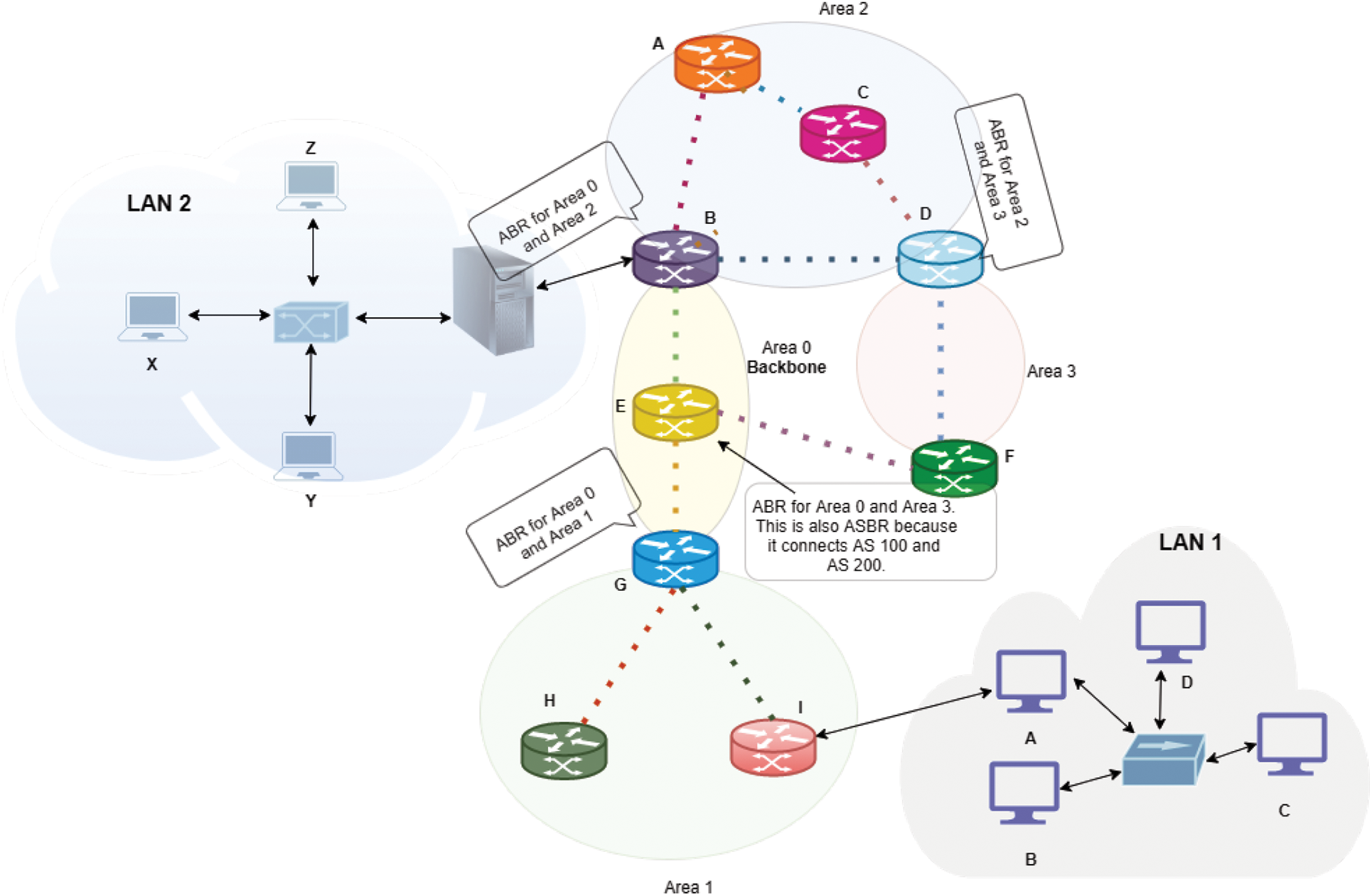
Figure 4: Hypothetical network layout

4.1 Best Path Selection in Computer Networks

Let us consider the same network situation as shown in Fig. 3. In the previous scenario, only one parameter is used for finding APSP, but now we used all network parameters and find APSP using our proposed algorithm. The considered parameters are length, bandwidth, delay, cost, MTU, throughput, hop count, load, and reliability. We know that the dynamics of the networks can not be the same all the time, they change according to network conditions which may results in a change of best path as well. If a path is best at any time t, it may be not best for the next moment if network dynamics change. Under such uncertain situations, PFS suits well to choose an appropriate path by considering ongoing network conditions. To understand the working of our algorithm in the said situation. We apply our proposed algorithm to find the best route among all possible options. Table 4 shows the TPFN that we are going to use in this example.

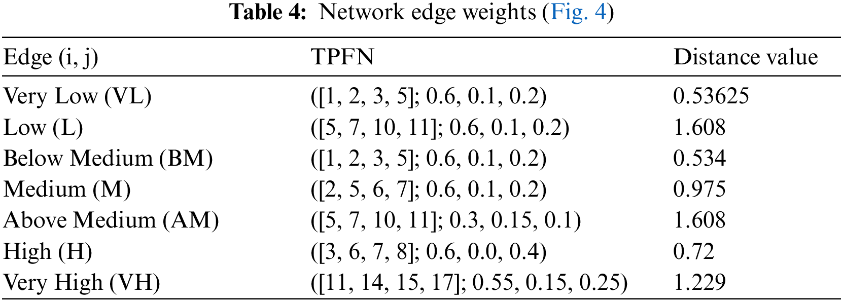
Table 5 shows the current situation of a network in linguistic terms. Each linguistic term corresponds to mentioned TPFN in Table 4.

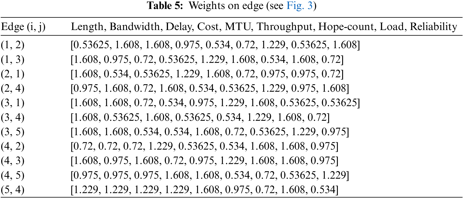
Iteration 0: The matrices A0 gives the initial representation of the network, where all (x,y)th entries of A0 are canonical representations of weights of route from x to y, and B0 respective sequence matrix (see page 19).

Iteration 1: Set k=1. The first row and column are treated as a pivot and their values remain the same from the previous matrices.

[2, 3] = [2, 1] + [1, 3] = [0.534, 1.608, 0.536, 1.229, 1.608, 0.72, 0.975, 0.975, 0.72] + [1.608, 0.975, 0.72, 0.536, 1.229, 0.534, 1.608, 1.608, 0.72] = [2.142, 2.583, 1.256, 1.765, 2.837, 1.254, 2.583, 2.583, 1.44] < [∞, ∞, ∞, ∞, ∞, ∞, ∞, ∞, ∞].

[2, 4] = [2, 1] + [1, 4] = [0.534, 1.608, 0.536, 1.229, 1.608, 0.72, 0.975, 0.975, 0.72] + [1.229, 0.72, 0.534, 0.975, 1.608, 1.608, 0.536, 0.534, 1.229] = [ 0.975, 1.608, 0.72, 0.534, 1.608, 0.536, 1.229, 0.975, 1.608] < [∞, ∞, ∞, ∞, ∞, ∞, ∞, ∞, ∞].

[2, 5] = [2, 1] + [1, 5] = [0.534, 1.608, 0.536, 1.229, 1.608, 0.72, 0.975, 0.975, 0.72 ] + [0.72, 1.608, 0.536, 0.975, 0.534, 1.608, 1.229, 1.608, 0.534] = [1.254, 3.216, 1.072, 2.204, 2.142, 2.328, 2.204, 2.583, 1.254] < [∞, ∞, ∞, ∞, ∞, ∞, ∞, ∞, ∞].

[3, 2] = [3, 1] + [1, 2] = [1.608, 0.534, 0.72, 1.608, 0.975, 1.229, 1.608, 0.536, 0.536] + [0.536, 1.608, 0.534, 0.975, 1.608, 0.72, 1.229, 0.536, 1.608] = [2.144, 2.142, 1.254, 2.583, 2.583, 1.949, 2.837, 1.072, 2.144] < [∞, ∞, ∞, ∞, ∞, ∞, ∞, ∞, ∞].

[3, 4] = [3, 1] + [1, 4] = [1.608, 0.534, 0.72, 1.608, 0.975, 1.229, 1.608, 0.536, 0.536] + [1.229, 0.72, 0.534, 0.975, 1.608, 1.608, 0.536, 0.534, 1.229] = [2.837, 1.254, 1.254, 2.583, 2.583, 1.949, 2.837, 1.072, 2.144] < [∞, ∞, ∞, ∞, ∞, ∞, ∞, ∞, ∞].

[3, 5] = [3, 1] + [1, 5] = [1.608, 0.534, 0.72, 1.608, 0.975, 1.229, 1.608, 0.536, 0.536] + [0.72, 1.608, 0.536, 0.975, 0.534, 1.608, 1.229, 1.608, 0.534] = [0.534, 0.534, 1.256, 1.608, 1.509, 0.72, 0.536, 1.229, 0.975] < [∞, ∞, ∞, ∞, ∞, ∞, ∞, ∞, ∞].

[4, 2] = [4, 1] + [1, 2] = [1.608, 1.608, 1.608, 0.72, 0.975, 0.536, 0.534, 1.608, 1.229] + [0.536, 1.608, 0.534, 0.975, 1.608, 0.72, 1.229, 0.536, 1.608] = [0.72, 0.72, 0.72, 1.229, 0.536, 1.256, 0.534, 1.608, 0.975] < [∞, ∞, ∞, ∞, ∞, ∞, ∞, ∞, ∞].

[4, 3] = [4, 1] + [1, 3] = [1.608, 1.608, 1.608, 0.72, 0.975, 0.536, 0.534, 1.608, 1.229] + [1.608, 0.975, 0.72, 0.536, 1.229, 0.534, 1.608, 1.608, 0.72] = [2.862, 2.583, 1.976, 1.256, 2.204, 1.070, 2.142, 3.216, 1.949] < [∞, ∞, ∞, ∞, ∞, ∞, ∞, ∞, ∞].

[4, 5] = [4, 1] + [1, 5] = [1.608, 1.608, 1.608, 0.72, 0.975, 0.536, 0.534, 1.608, 1.229] + [0.72, 1.608, 0.536, 0.975, 0.534, 1.608, 1.229, 1.608, 0.534] = [0.975, 0.975, 0.975, 1.608, 0.534, 1.608, 0.72, 0.536, 1.229] < [∞, ∞, ∞, ∞, ∞, ∞, ∞, ∞, ∞].

[5, 2] = [5, 1] + [1, 2] = [0.536, 1.229, 1.608, 0.72, 0.536, 1.229, 0.534, 1.608, 0.975] + [0.536, 1.608, 0.534, 0.975, 1.608, 0.72, 1.229, 0.536, 1.608] = [1.072, 2.831, 2.142, 1.695, 2.144, 1.949, 1.763, 2.144, 2.583] < [∞, ∞, ∞, ∞, ∞, ∞, ∞, ∞, ∞].

[5, 3] = [5, 1] + [1, 3] = [0.536, 1.229, 1.608, 0.72, 0.536, 1.229, 0.534, 1.608, 0.975] + [1.608, 0.975, 0.72, 0.536, 1.229, 0.534, 1.608, 1.608, 0.72] = [0.534, 1.608, 1.229, 0.536, 0.536, 1.229, 1.608, 0.975, 0.72] < [∞, ∞, ∞, ∞, ∞, ∞, ∞, ∞, ∞].

[5, 4] = [5, 1] + [1, 4] = [0.536, 1.229, 1.608, 0.72, 0.536, 1.229, 0.534, 1.608, 0.975] + [1.229, 0.72, 0.534, 0.975, 1.608, 1.608, 0.536, 0.534, 1.229] = [1.229, 1.229, 1.229, 1.095, 1.608, 0.975, 0.72, 0.534, 1.604] < [∞, ∞, ∞, ∞, ∞, ∞, ∞, ∞, ∞].

Now set k=2 in the next iteration. The second row and second column in the matrix, A2 are set as pivot row and pivot column, and their values have no change from the previous matrices. Now perform calculations as we did in iteration 1. A total of five iterations would be done with k=3, k=4, and k=5. Table 6 shows the final findings of our algorithms after five iterations.

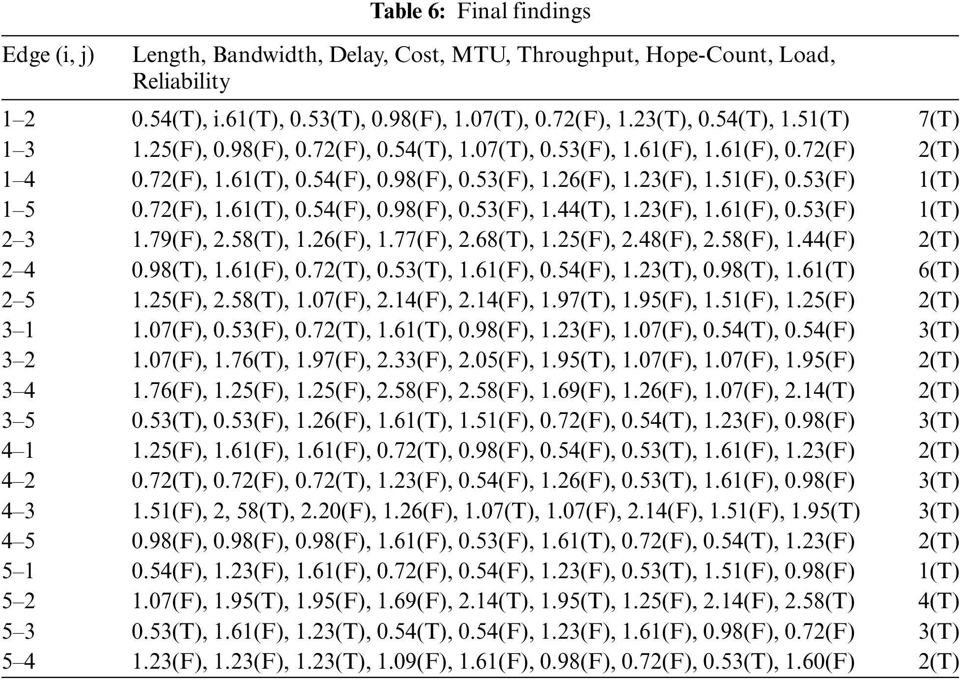
As we can see the shortest path from node 1 to 5 is 1→2→4→5.

[(0,0,0,0,0,0,0,0,0)(0.54,1.61,0.53,0.98,1.61,0.72,1.23,0.54,1.61)(0.53,1.61,0.54,1.23,1.61,0.72,0.98,0.98,0.72)(0,0,0,0,0,0,0,0,0)(1.61,0.53,0.72,1.61,0.98,1.23,1.61,0.54,0.54)(∞,∞,∞,∞,∞,∞,∞,∞,∞)(1.61,1.61,1.61,0.72,0.98,0.54,0.53,1.61,1.23)(0.72,0.72,0.72,1.23,0.54,1.61,0.53,1.61,0.98)(0.54,1.23,1.61,0.72,0.54,1.23,0.53,1.61,0.98)(∞,∞,∞,∞,∞,∞,∞,∞,∞)A0=(1.61,0.98,0.72,0.54,1.23,0.53,1.61,1.61,0.72)(1.23,0.72,0.53,0.98,1.61,1.61,0.54,0.53,1.23)(∞,∞,∞,∞,∞,∞,∞,∞)(0.98,1.61,0.72,0.53,1.61,0.54,1.23,0.98,1.61)(0,0,0,0,0,0,0,0,0)(∞,∞,∞,∞,∞,∞,∞,∞)(∞,∞,∞,∞,∞,∞,∞,∞,∞)(0,0,0,0,0,0,0,0,0)(0.53,1.61,1.23,0.54,0.54,1.23,1.61,0.98,0.72)(1.23,1.23,1.23,1.23,1.61,0.98,0.72,0.53,1.61)(0.72,1.61,0.54,0.98,0.53,1.61,1.23,1.61,0.53)(∞,∞,∞,∞,∞,∞,∞,∞,∞)(0.53,0.53,1.61,1.61,1.61,0.72,0.54,1.23,0.98)(0.98,0.98,0.98,1.61,0.53,1.61,0.72,0.54,1.23)(0,0,0,0,0,0,0,0,0)]

[(0,0,0,0,0,0,0,0,0)(0.54,1.61,0.53,0.98,1.61,0.72,1.23,0.54,1.61)(0.53,1.61,0.54,1.23,1.61,0.72,0.98,0.98,0.72)(0,0,0,0,0,0,0,0,0)(1.61,0.53,0.72,1.61,0.98,1.23,1.61,0.54,0.54)(2.14,2.142,1.25,2.58,2.58,1.95,2.84,1.07,2.14)(1.61,1.61,1.61,0.72,0.98,0.54,0.53,1.61,1.23)(0.72,0.72,0.72,1.23,0.54,1.26,0.53,1.61,0.98)(0.54,1.23,1.61,0.72,0.54,1.23,0.53,1.61,0.98)(1.07,2.83,2.14,1.60,2.14,1.95,1.76,2.14,2.58)A1=(1.61,0.98,0.72,0.54,1.23,0.53,1.61,1.61,0.72)(1.23,0.72,0.53,0.98,1.61,1.61,0.54,0.53,1.23)(2.14,2.58,1.26,1.77,2.84,1.25,2.58,2.58,1.44)(0.98,1.61,0.72,0.53,1.61,0.54,1.23,0.98,1.61)(0,0,0,0,0,0,0,0,0)(2.84,1.25,1.25,2.58,2.58,1.95,2.84,1.07,2.14)(2.86,2.58,1.98,1.26,2.20,1.07,2.14,3.22,1.95)(0,0,0,0,0,0,0,0,0)(0.53,1.61,1.23,0.54,0.54,1.23,1.61,0.98,0.72)(1.23,1.23,1.23,1.09,1.61,0.98,0.72,0.53,1.60)(0.72,1.61,0.54,0.98,0.53,1.61,1.23,1.61,0.53)(1.25,3.22,1.07,2.20,2.14,2.33,2.20,2.58,1.25)(0.53,0.53,1.26,1.61,1.51,0.72,0.54,1.23,0.98)(0.98,0.98,0.98,1.61,0.53,1.61,0.72,0.54,1.23)(0,0,0,0,0,0,0,0,0)]

[(0,0,0,0,0,0,0,0,0)(0.54,1.61,0.53,0.98,1.61,0.72,1.23,0.54,1.61)(0.53,1.61,0.54,1.23,1.61,0.72,0.98,0.98,0.72)(0,0,0,0,0,0,0,0,0)(1.61,0.53,0.72,1.61,0.98,1.23,1.61,0.54,0.54)(2.14,2.14,1.25,2.58,2.58,1.95,2.84,1.07,2.14)(1.25,1.61,1.61,0.72,0.98,0.54,0.53,1.61,1.23)(0.72,0.72,0.72,1.23,0.54,1.26,0.53,1.61,0.98)(0.54,1.23,1.61,0.72,0.54,1.23,0.53,1.61,0.98)(1.07,2.83,2.14,1.69,2.14,1.95,1.76,2.14,2.58)A2=(1.61,0.98,0.72,0.54,1.23,0.53,1.61,1.61,0.72)(0.72,1.61,0.54,0.98,0.53,1.26,1.23,1.51,0.53)(2.14,2.58,1.26,1.77,2.84,1.25,2.58,2.58,1.44)(0.98,1.61,0.72,0.53,1.61,0.54,1.23,0.98,1.61)(0,0,0,0,0,0,0,0,0)(2.84,1.25,1.25,2.58,2.58,1.95,2.84,1.07,2.14)(3.22,2.58,2.33,1.26,2.20,1.07,2.14,3.22,1.95)(0,0,0,0,0,0,0,0,0)(0.53,1.61,1.23,0.54,0.54,1.23,1.61,0.98,0.72)(1.23,1.23,1.23,1.09,1.61,0.98,0.72,0.53,1.60)(0.72,1.61,0.54,0.98,0.53,1.61,1.23,1.61,0.53)(1.25,3.22,1.1.07,2.20,2.14,2.33,2.20,2.58,1.25)(0.53,0.53,1.26,1.61,1.51,0.72,0.54,1.23,0.98)(0.98,0.98,0.98,1.61,0.53,1.61,0.72,0.54,1.23)(0,0,0,0,0,0,0,0,0)],

[(0,0,0,0,0,0,0,0,0)(0.54,1.61,0.53,0.98,1.61,0.72,1.23,0.54,1.61)(0.53,1.61,0.54,1.23,1.61,0.72,0.98,0.98,0.72)(0,0,0,0,0,0,0,0,0)(1.61,0.53,0.72,1.61,0.98,1.23,1.61,0.54,0.54)(2.14,2.142,1.25,2.58,2.58,1.95,2.84,1.07,2.14)(1.25,1.61,1.61,0.72,0.98,0.54,0.53,1.61,1.23)(0.72,0.72,0.72,1.23,0.54,1.26,0.53,1.61,0.98)(0.54,1.23,1.61,0.72,0.54,1.23,0.53,1.51,0.98)(1.07,1.95,1.95,1.69,2.14,1.95,1.76,2.14,2.58)A3=(1.61,0.98,0.72,0.54,1.23,0.53,1.61,1.61,0.72)(0.72,1.61,0.54,0.98,0.53,1.26,1.23,1.51,0.53)(2.14,2.58,1.26,1.77,2.84,1.25,2.58,2.58,1.44)(0.98,1.61,0.72,0.53,1.61,0.54,1.23,0.98,1.61)(0,0,0,0,0,0,0,0,0)(2.84,1.25,1.25,2.58,2.58,1.95,2.84,1.07,2.14)(3.22,2.58,2.33,1.26,2.20,1.07,2.14,3.22,1.95)(0,0,0,0,0,0,0,0,0)(0.53,1.61,1.23,0.54,0.54,1.23,1.61,0.98,0.72)(1.23,1.23,1.23,1.09,1.61,0.98,0.72,0.53,1.60)(0.72,1.61,0.54,0.98,0.53,1.44,1.23,1.61,0.53)(1.25,3.22,1.07,2.20,2.14,1.97,2.20,2.58,1.25)(0.53,0.53,1.26,1.61,1.51,0.72,0.54,1.23,0.98)(0.98,0.98,0.98,1.61,0.53,1.61,0.72,0.53,1.23)(0,0,0,0,0,0,0,0,0)],

[(0,0,0,0,0,0,0,0,0)(0.54,1.61,0.53,0.98,1.07,0.72,1.23,0.54,1.51)(0.53,1.61,0.54,1.23,1.61,0.72,0.98,0.98,0.72)(0,0,0,0,0,0,0,0,0)(1.61,0.53,0.72,1.61,0.98,1.23,1.61,0.54,0.54)(2.14,1.97,1.97,2.58,2.58,1.95,2.84,1.07,2.14)(1.25,1.61,1.61,0.72,0.98,0.54,0.53,1.61,1.23)(0.72,0.72,0.72,1.23,0.54,1.26,0.53,1.61,0.98)(0.54,1.23,1.61,0.72,0.54,1.23,0.53,1.51,0.98)(1.073,1.95,1.95,1.69,2.14,1.95,1.25,2.14,2.58)A4=(1.61,0.98,0.72,0.54,1.23,0.53,1.61,1.61,0.72)(0.72,1.61,0.54,0.98,0.53,1.26,1.23,1.51,0.53)(2.14,2.58,1.26,1.77,2.84,1.25,2.58,2.58,1.44)(0.98,1.61,0.72,0.53,1.61,0.54,1.23,0.98,1.61)(0,0,0,0,0,0,0,0,0)(2.84,1.25,1.25,2.58,2.58,1.95,2.84,1.07,2.14)(3.22,2.58,2.33,1.26,2.20,1.07,2.14,3.22,1.95)(0,0,0,0,0,0,0,0,0)(0.53,1.61,1.23,0.54,0.54,1.23,1.61,0.98,0.72)(1.23,1.23,1.23,1.09,1.61,0.98,0.72,0.53,1.60)(0.72,1.61,0.54,0.98,0.53,1.44,1.23,1.61,0.53)(1.25,2.58,1.07,2.14,2.14,1.97,1.95,1.51,1.25)(0.53,0.53,1.26,1.61,1.51,0.72,0.53,1.23,0.98)(0.98,0.98,0.98,1.61,0.53,1.61,0.72,0.54,1.23)(0,0,0,0,0,0,0,0,0)],

[(0,0,0,0,0,0,0,0,0)(0.54,1.61,0.53,0.98,1.07,0.72,1.23,0.54,1.51)(0.53,1.61,0.54,1.23,1.61,0.72,0.98,0.98,0.72)(0,0,0,0,0,0,0,0,0)(0.07,0.53,0.72,1.61,0.98,1.23,1.07,0.54,0.54)(1.07,1.76,1.97,2.33,2.05,1.95,1.07,1.07,1.95)(1.25,1.61,1.61,0.72,0.98,0.54,0.53,1.61,1.23)(0.72,0.72,0.72,1.23,0.54,1.24,0.53,1.61,0.98)(0.54,1.23,1.61,0.72,0.54,1.23,0.53,1.51,0.98)(1.07,1.95,1.95,1.7,2.14,1.95,1.25,2.14,2.58)A5=(1.25,0.98,0.72,0.54,1.07,0.53,1.61,1.61,0.72)(0.72,1.61,0.54,0.98,0.53,1.26,1.23,1.51,0.53)(1.79,2.58,1.26,1.77,2.68,1.25,2.48,2.58,1.44)(0.98,1.61,0.72,0.53,1.61,0.54,1.23,0.98,1.61)(0,0,0,0,0,0,0,0,0)(1.76,1.25,1.25,2.58,2.58,1.7,1.26,1.07,2.14)(1.51,2.58,2.2,1.26,1.07,1.07,2.14,1.51,1.95)(0,0,0,0,0,0,0,0,0)(0.53,1.61,1.23,0.54,0.54,1.23,1.61,0.98,0.72)(1.23,1.23,1.23,1.1,1.61,0.98,0.72,0.53,1.60)(0.72,1.61,0.54,0.98,0.53,1.44,1.23,1.61,0.53)(1.25,2.58,1.07,2.14,2.14,1.97,1.95,1.51,1.25)(0.53,0.53,1.26,1.61,1.51,0.72,0.54,1.23,0.98)(0.98,0.98,0.98,1.61,0.53,1.61,0.72,0.54,1.23)(0,0,0,0,0,0,0,0,0)].

              01   02   03  04  05B0=12345(0234510345120451230512340)              01   02   03  04  05B1=12345(0234510141110151210511340)              01   02   03  04  05B2=12345(0232510141110151220511340)              01   02   03  04  05B3=12345(0232310143110151220513340)              01   02   03  04  05B4=12345(0432310144140151220514340)              01   02   03  04  05B5=12345(0452310544550551250514340)

5  Comparative Analysis

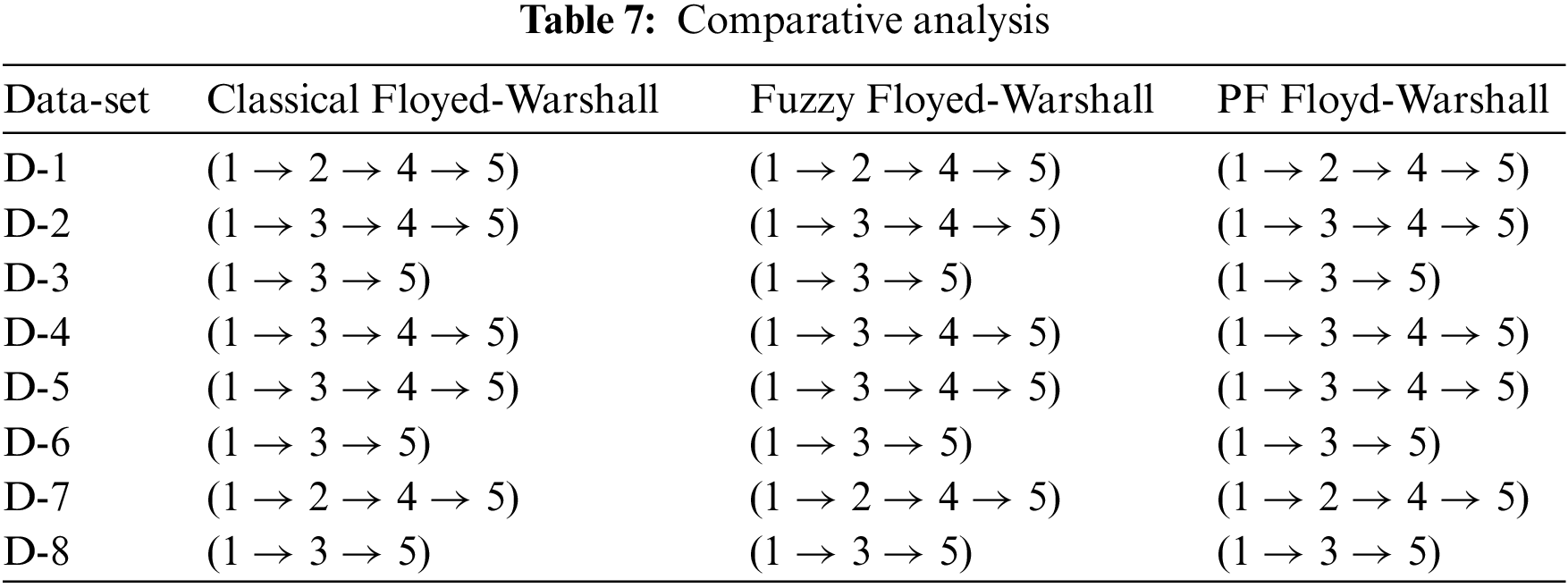
In this section, we provide a brief comparative analysis of the proposed algorithm with the classical Floyd-Warshall and fuzzy Floyd-Warshall algorithms. The classical Floyd-Warshall algorithm and fuzzy Floyd-Warshall algorithm take only one input parameter and decide the best route. But, in actual scenarios, multiple input factors may involve. In such scenarios, the previous techniques fail to take any decision. Whereas in the proposed method, we can work with n number of factors that may influence the final decision. For testing our model, we considered eight hypothetical data sets and applied PF Floyd-Warshall, fuzzy Floyd-Warshall, and the classical Floyd-Warshall algorithm. First of all, the picture fuzzy Floyd-Warshall algorithm calculates the distance between each pair using the score function of TPFN. Set the distance value to infinity if there is no direct connection found in the graph or network. Now consider the breaking point k which lies between 1 to n and check for each value of k if the distance of any pair of nodes passing through this breaking point is less than the previously defined distance, replace it with the new distance. If any criteria of a factor meet, assign true against that criteria. Lastly, choose one best path which is having maximum true values. We observed that all of the considered methods highlighted the same results against the same data sets, which proved the authenticity of our work. Table 7 shows the results of the comparative analysis. The first column is labeled as a graph. The data set is in the form of a Graph. We have taken the same graph as shown in Fig. 3 but with different edge weights. The second, third, and fourth columns show the results obtained from the classical Floyd-Warshall algorithm, fuzzy Floyd-Warshall algorithm, and picture fuzzy Floyd-Warshall algorithm, respectively. Table 7 shows the comparison of different Floyd-Warshall algorithms.

6  Conclusion and Future Directions

PFS is a useful and powerful tool to represent human opinion in terms of yes, abstain, no, and refusal. It gives more degrees of freedom than an intuitionistic fuzzy set (IFS). In short words, PFS is the generalized form of IFS. In this paper, we used PFN to find APSP using the Floyd-Warshall algorithm. The weights on each edge are defined as a PFN, and the distance between any two vertices is calculated using the expected value and score functions of PFN. Then we used triple operation to compare any two distances. This article has presented a new variant of the Floyd-Warshall algorithm to compute APSP. The picture fuzzy Floyd-Warshall algorithm incrementally finds APSP with the help of intermediate nodes. The time complexity of the proposed algorithm is O(n3). We have also compared our proposed algorithm with the classical fuzzy Floyd-Warshall and fuzzy Floyd-Warshall algorithms. All algorithms highlighted the same path for any pair of vertices. The proposed approach can be applied to many real-life problems, some of which are discussed below:

•   The proposed method can be applied to find the fastest route for ambulance services.

•   The proposed methodology can be used to locate the best route in the transportation network. The route depends on many factors, for example, construction activity, distance, fuel consumption, traffic situation, and many others.

•   In medicine, different experts have different opinions about any treatment. Our proposed method helps to choose the most weighted opinion out of all opinions. The weight of each may depend on the qualification and experience of the expert, the cost of treatment, etc.

•   Floyd-Warshall algorithm can be used to evaluate victim route planning.

•   Information-Centric Network (ICN) heavily depends on the internet to perform information-related activities, like information access and delivery. Sometimes, we face cache overlap problems. To handle such problems, we can use the picture fuzzy Floyd-Warshall algorithm to find the shortest path in each subnet for retrieving the cache memory data quickly and removing invalid routes.

Funding Statement: The authors extend their appreciation to the Deanship of Scientific Research at King Khalid University for funding this work through General Research Project under Grant No. (R.G.P.2/48/43).

Ethics Approval: This article does not contain any studies with human participants or animals performed by the author.

Conflicts of Interest: The authors declare that they have no conflicts of interest to report regarding the present study.

References

1. Zadeh, L. A. (1965). Fuzzy sets. Information and Control, 8(3), 338–353. https://doi.org/10.1016/S0019-9958(65)90241-X [Google Scholar] [CrossRef]

2. Atanassov, K. T. (1986). Intuitionistic fuzzy sets: Theory and applications. Fuzzy Sets and System, 20, 87–96. https://doi.org/10.1016/S0165-0114(86)80034-3 [Google Scholar] [CrossRef]

3. Cuong, B. C. (2013). Picture fuzzy sets-first results. Seminar on Neuro-fuzzy systems with applications, Institute of Mathematics, Vietnam Academy of Science and Technology, Hanoi, Vietnam. [Google Scholar]

4. Cuong, B. C., Kreinovich, V. (2013). Picture fuzzy sets–A new concept for computational intelligence problems. 2013 Third World Congress on Information and Communication Technologies (WICT), pp. 1–6. Hanoi, Vietnam. https://doi.org/10.1109/WICT.2013.7113099 [Google Scholar] [CrossRef]

5. Wan, S. P., Yi, Z. H. (2016). Power average of trapezoidal intuitionistic fuzzy numbers using strict t-norms and t-conorms. IEEE Transactions on Fuzzy Systems, 24(5), 1035–1047. https://doi.org/10.1109/TFUZZ.2015.2501408 [Google Scholar] [CrossRef]

6. Dubois, D., Prade, H. (1980). Fuzzy sets and systems: Theory and applications, vol. 144. Amsterdam: Academic Press. [Google Scholar]

7. Okada, S., Gen, M. (1994). Fuzzy shortest path problem. Computers & Industrial Engineering, 27, 465–468. https://doi.org/10.1016/0360-8352(94)90335-2 [Google Scholar] [CrossRef]

8. Mahdavi, I., Nourifar, R., Heidarzade, A., Amiri, N. M. (2009). A dynamic programming approach for finding shortest chains in a fuzzy network. Applied Soft Computing, 9(2), 503–511. 110.1016/j.asoc.2008.07.002 [Google Scholar]

9. Dou, Y., Zhu, L., Wang, H. S. (2012). Solving the fuzzy shortest path problem using multi-criteria decision method based on vague similarity measure. Applied Soft Computing, 12(6), 1621–1631. https://doi.org/10.1016/j.asoc.2012.03.013 [Google Scholar] [CrossRef]

10. Tajdin, A., Mahdavi, I., Mahdavi-Amiri, N., Sadeghpour-Gildeh, B. (2010). Computing a fuzzy shortest path in a network with mixed fuzzy arc lengths using α-cuts. Computers & Mathematics with Applications, 60(4), 989–1002. https://doi.org/10.1016/j.camwa.2010.03.038 [Google Scholar] [CrossRef]

11. Dey, A., Pradhan, R., Pal, A., Pal, T. (2018). A genetic algorithm for solving fuzzy shortest path problems with interval type-2 fuzzy arc lengths. Malaysian Journal of Computer Science, 31(4), 255–270. https://doi.org/10.22452/mjcs [Google Scholar] [CrossRef]

12. Garg, H., Rawat, P. (2012). An improved algorithm for finding all pair shortest path. International Journal of Computer Applications, 47(25), 35–37. https://doi.org/10.5120/7539-0492 [Google Scholar] [CrossRef]

13. Shukla, K. T. (2013). Fuzzy floyd’s algorithm to find shortest route between nodes under uncertain environment. International Journal of Mathematics and Computer Applications Research, 3(5), 43–54. [Google Scholar]

14. Aziz, A., Farid, M. M., Suryani, E. (2017). Floyd warshall algorithm with FIS sugeno for search evacuation route optimization. International Seminar on Application for Technology of Information and Communication (iSemantic), pp. 147–151. Semarang, Indonesia. https://doi.org/10.1109/ISEMANTIC.2017.8251860 [Google Scholar] [CrossRef]

15. Shafahi, Y., Faturechi, R. (2009). A new fuzzy approach to estimate the O-D matrix from link volumes. Transportation Planning and Technology, 32(6), 499–526. https://doi.org/10.1080/03081060903374700 [Google Scholar] [CrossRef]

16. Broumi, S., Talea, M., Bakali, A., Smarandache, F., Nagarajan, D. et al. (2019). Shortest path problem in fuzzy, intuitionistic fuzzy and neutrosophic environment: An overview. Complex & Intelligent Systems, 5(4), 371–378. https://doi.org/10.1007/s40747-019-0098-z [Google Scholar] [CrossRef]

17. Akram, M., Habib, A., Alcantud, J. C. R. (2021). An optimization study based on dijkstra algorithm for a network with trapezoidal picture fuzzy numbers. Neural Computing and Applications, 33, 1329–1342. https://doi.org/10.1007/s00521-020-05034-y [Google Scholar] [CrossRef]

18. Akram, M., Shahzadi, G., Alcantud, J. C. R. (2022). Multi-attribute decision-making with q-rung picture fuzzy information. Granular Computing, 7, 197–215. https://doi.org/10.1007/s41066-021-00260-8 [Google Scholar] [CrossRef]

19. Akram, M., Bashir, A., Edalatpanah, S. A. (2021). A hybrid decision-making analysis under complex q-rung picture fuzzy einstein averaging operators. Computational and Applied Mathematics, 40(8), 1–35. https://doi.org/10.1007/s40314-021-01651-y [Google Scholar] [CrossRef]

20. Akram, M., Ullah, I., Allahviranloo, T. (2022). A new method to solve linear programming problems in the environment of picture fuzzy sets. Iranian Journal of Fuzzy Systems, 19(6), 29–49. https://doi.org/10.22111/ijfs.2022.7208 [Google Scholar] [CrossRef]

21. Thao, N. X. (2020). Similarity measures of picture fuzzy sets based on entropy and their application in MCDM. Pattern Analysis and Applications, 23(3), 1203–1213. https://doi.org/10.1007/s10044-019-00861-9 [Google Scholar] [CrossRef]

22. Mahmood, T., Ali, Z. (2020). The fuzzy cross-entropy for picture hesitant fuzzy sets and their application in multi citeria decision making. Punjab University Journal of Mathematics, 52(10), 55–82. ISSN 1016-2526. [Google Scholar]

23. Ganie, A. H., Singh, S., Bhatia, P. K. (2020). Some new correlation coefficients of picture fuzzy sets with applications. Neural Computing and Applications, 32(16), 12609–12625. https://doi.org/10.1007/s00521-020-04715-y [Google Scholar] [CrossRef]

24. Nirmani, A., Thilakarathne, L., Wickramasinghe, A., Senanayake, S., Haddela, P. S. (2018). Google map and camera based fuzzified adaptive networked traffic light handling model. 3rd International Conference on Information Technology Research (ICITR), pp. 1–6. Institute of Electrical and Electronics Engineers Inc., Moratuwa, Sri Lanka. https://doi.org/10.1109/ICITR.2018.8736158 [Google Scholar] [CrossRef]

25. Yue, Q. (2022). Bilateral matching decision-making for knowledge innovation management considering matching willingness in an interval intuitionistic fuzzy set environment. Journal of Innovation & Knowledge, 7(3), 100209. https://doi.org/10.1016/j.jik.2022.100209 [Google Scholar] [CrossRef]

26. Jiang, Z., Wei, G., Guo, Y. (2022). Picture fuzzy MABAC method based on prospect theory for multiple attribute group decision making and its application to suppliers selection. Journal of Intelligent & Fuzzy Systems, 42(4), 3405–3415. https://doi.org/10.3233/JIFS-211359 [Google Scholar] [CrossRef]

27. Habib, S., Akram, M., Al-Shamiri, M. M. A. (2023). Comparative analysis of pythagorean MCDM methods for the risk assessment of childhood cancer. Computer Modeling in Engineering & Sciences, 135(3), 2585–2615. https://doi.org/10.32604/cmes.2023.024551 [Google Scholar] [CrossRef]

28. Akram, M., Habib, A., Allahviranloo, T. (2022). A new maximal flow algorithm for solving optimization problems with linguistic capacities and flows. Information Sciences, 612, 201–230. https://doi.org/10.1016/j.ins.2022.08.068 [Google Scholar] [CrossRef]

29. Habib, A., Akram, M., Kahraman, C. (2022). Minimum spanning tree hierarchical clustering algorithm: A new pythagorean fuzzy similarity measure for the analysis of functional brain networks. Expert Systems with Applications, 201, 117016. https://doi.org/10.1016/j.eswa.2022.117016 [Google Scholar] [CrossRef]

30. Zhang, F., Zhao, Y., Ye, J., Wang, S., Hu, J. (2023). Novel distance measures on hesitant fuzzy sets based on equal-probability transformation and their application in decision making on intersection traffic control. Computer Modeling in Engineering & Sciences, 135(2), 1589–1602. https://doi.org/10.32604/cmes.2022.022431 [Google Scholar] [CrossRef]

31. Zhang, F., Xu, S., Han, B., Zhang, L., Ye, J. (2023). Neutrosophic adaptive clustering optimization in genetic algorithm and its application in cubic assignment problem. Computer Modeling in Engineering & Sciences, 134(3), 2211–2226. https://doi.org/10.32604/cmes.2022.022418 [Google Scholar] [CrossRef]

32. Yi, Y., Guan, Y. (2012). A path planning method to robot soccer based on dijkstra algorithm. In: Jin, D., Lin, S. (Eds.Advances in electronic commerce, web application and communication, pp. 89–95. https://doi.org/10.1007/978-3-642-28658-2_14 [Google Scholar] [CrossRef]

33. Zadeh, L. A. (1975). The concept of a linguistic variable and its application to approximate reasoning–I. Information Sciences, 8(3), 199–249. https://doi.org/10.1016/0020-0255(75)90036-5 [Google Scholar] [CrossRef]

34. Zulqarnain, R. M., Siddique, I., Iampan, A., Baleanu, D. (2022). Aggregation operators for interval-valued pythagorean fuzzy soft set with their application to solve multi-attribute group decision making problem. Computer Modeling in Engineering & Sciences, 131(3), 1717–1750. https://doi.org/10.32604/cmes.2022.019408 [Google Scholar] [CrossRef]