ABAQUS and ANSYS Implementations of the Peridynamics-Based Finite Element Method (PeriFEM) for Brittle Fractures

1  Introduction

Establishing mathematical models for natural phenomena is the second paradigm in the scientific investigation [1]. More specifically, in the engineering and physics fields, many problems are traditionally summarized as a (group of) partial differential equation(s). However, the analytical solutions of these equations are usually difficult to obtain, and thus, we have to rely on numerical methods [2]. The finite element method (FEM) is one of the most popular numerical methods due to its standardized analysis process and applicability to a wide variety of problems.

However, the development of the FEM has not been smooth sailing, and it is said that even a well-known journal at that time shunned papers on the finite element method for many years [3]. In the 1960s, things turned around benefiting from Ed Wilson’s liberal distribution of his first programs, making more and more people realize the value of the FEM and devote themselves to this field. Then in the next few decades, numerous FEM software sprang up, which greatly promoted the application of the FEM in engineering practice. In particular, commercial FEM software uses interactive windows to make applications more convenient and their appearance also makes the finite element analysis easier.

With the development of cutting-edge science and technologies over the past few years, the service environment of engineering structures has become increasingly complicated, and their analysis is facing new challenges, such as fracture. For these challenges, traditional commercial FEM software is probably to be ineffective. There are two main strategies to approach these problems: (1) developers integrate advanced techniques into the software directly or (2) users incorporate advanced techniques into the software using a programmable interface. The first option may be more suitable for more mature technology because software development is expensive in terms of time and funding. The second option is better able to adapt to the most advanced techniques and accumulate experience for the first option. For example, before ABAQUS launched a version containing the extended finite element method (XFEM), Fang et al. [4] had implemented XFEM simulations in it. For other methods that have received widespread attention, such as the cohesive zone model and the phase field model of fracture [5,6], there are also related works in which these methods were implemented in existing software. For example, Lindgaard et al. [7] presented a cohesive zone finite element method implemented via user programmable features (UPFs) in ANSYS; and Msekh et al. [8–10] incorporated the phase field model of fracture with ABAQUS via subroutines.

Peridynamics has also attracted considerable research attention as a new non-local theory [11,12], and has been applied to many engineering problems, such as the stress analysis in the vicinity of the crack tip [13], fracture modelling of reinforced concrete [14,15], and the inelastic fracture [16], etc. The governing equations in peridynamics are integral–differential equations rather than partial differential equations. Therefore, discontinuities are naturally tolerated, which offers considerable advantages when simulating fracture problems. Thus, incorporating peridynamics into commercial FEM software could considerably promote its engineering applications. However, because of the integration aspect of peridynamic equations, only a few studies have used element-based methods to solve them [17–19]; most studies use particle-based methods that can directly approximate the integration as a Riemann summation [20–22], which is hardly compatible with commercial FEM software. To the best of the authors’ knowledge, only a few studies have implemented peridynamics in commercial FEM software [23–26]. Diyaroglu et al. [23] used a truss element to present the peridynamic bond [27], and peridynamics simulations were implemented in ANSYS. Huang et al. [24] defined the collection of all peridynamic particles in a horizon as a new element and conducted peridynamics simulations in ABAQUS. However, this type of element is undefined around the boundary, and thus a coupled model had to be used. Bie et al. [25] overcame the aforementioned problems around the boundary and implemented dual peridynamics in ABAQUS. However, they had to define many types of elements. Anicode et al. [26] used native MATRIX27 elements to perform peridynamic analysis in ANSYS. Notably, in existing reports, although peridynamics was implemented in FEM software, most of them used particles and regular grid for spatial discretization. On the other hand, an element-based implementation of peridynamics in commercial FEM software is still inadequate, particularly with irregular meshes. To our knowledge, Ren et al. [28,29] achieved the element-based peridynamics through a packaged peridynamic module in LS-DYNA. In this work, we consider the implementation based on the Application Programming Interface (API) of the software, which will be beneficial to the users for their specific requirements.

In this study, we propose a unified implementation technique for peridynamics in commercial FEM software based on the peridynamics-based finite element method (PeriFEM) [30,31]. PeriFEM was established in [30], and in [31], an adaptive continuous/discrete element technique was proposed as a supplement to [30]. However, both Han et al. [30] and Li et al. [31] employed an in-house code. In contrast, in this work, we concentrate on the implementation of PeriFEM in commercial FEM software based on its application programming interface (API) [32], which should be beneficial to users by better adapting to their specific requirements. PeriFEM is an element-based method in which only two types of elements are required. More importantly, the computational framework of PeriFEM is consistent with that of traditional FEM; thus, it can be conveniently implemented in any commercial FEM software with a programmable interface. Therefore, we implemented peridynamics simulations in ANSYS and ABAQUS using PeriFEM. The implementation process in these two pieces of software is similar, which shows that PeriFEM can be easily extended to other commercial FEM software packages. In addition, two different convergence criteria for the implicit iteration process are used in ANSYS and ABAQUS.

The rest of this paper is organized as follows. Section 2 reviews the basic formulations of bond-based peridynamics. Section 3 introduces PeriFEM in detail, including the definition of elements, shape functions, and establishment of linear equations. Section 4 is devoted to the numerical algorithm of PeriFEM and two convergence criteria. Section 5 describes the implementation of PeriFEM in ANSYS and ABAQUS. Numerical examples are presented in Section 6 to verify the proposed algorithms and programs. Finally, conclusions are drawn in Section 7.

2  Review of Peridynamics

Peridynamics is a reformulation of elasticity theory for discontinuities and long-range forces [11], which assumes that a point in the peridynamic continuum can interact with all points in its neighborhood through bonds. According to the mode of action of the force associated with the bonds, peridynamic formulations can be classified into bond-based and state-based peridynamics [12]. Here, we focus on the first one in the quasi-static case, and all mentions of “peridynamics” in subsequent sections refer to bond-based peridynamics.

Similar to classical elasticity theory, there are three groups of basic equations in peridynamics, i.e., the equilibrium, constitutive, and kinematic equations. These can be respectively expressed as

∫Hδ(x)f(ξ)dVξ+b(x)=0,∀x∈Ω,(1a)

f(ξ)=C(ξ)⋅η(ξ),∀x′∈Hδ(x),x∈Ω,(1b)

η(ξ)=u(x′)−u(x),∀x′,x∈Ω,(1c)

where Ω⊂Rd (d=1,2,3) is the reference configuration, x and x′ are points in Ω, Hδ(x) is the neighborhood of point x with a cut-off radius δ, b(x) is the external body force, ξ=x′−x is a relative position vector referred to as a bond, and η(ξ) and f(ξ) are the measure of deformation and the pairwise force vector of bond ξ, respectively. In addition to these basic equations, there are displacement boundary conditions in peridynamics, which can be expressed as

u(x)=u∗(x),∀x∈∂Ωu,(2)

here, ∂Ωu refers to a part of the boundary of Ω where a prescribed displacement is applied. In addition, traction boundary conditions are not considered directly in peridynamics [33].

C(ξ) in Eq. (1b) is the micro-modulus tensor, which is defined as [11]

C(ξ)=c(ξ)ξ⊗ξ,(3)

where c(ξ) denotes the micro-modulus coefficient. Furthermore, c(ξ) can be multiplicatively decomposed into a bond length-related part c^(‖ξ‖) and a non-related part c~(θ,φ) (where θ and φ are the polar and azimuthal angles of ξ in spherical coordinates, respectively), i.e.,

c(ξ)=c^(‖ξ‖)c~(θ,φ),(4)

where c^(‖ξ‖) can be a function of ‖ξ‖ in the form of a constant (e.g., c^(‖ξ‖)=1 [21]), linear (e.g., c^(‖ξ‖)=1−‖ξ‖/δ [34]), or exponential function (e.g., c^(‖ξ‖)=e−‖ξ‖/l [35], where l is a characteristic length related to the fracture process zone, see [36]), among others. Here, we adopted an exponential function. c~(θ,φ) can be determined according to the deformation energy equivalence between peridynamics and classical continuum mechanics. For isotropic materials, c~(θ,φ) degenerates to a constant c~0 related to Young’s modulus E, i.e.,

c~(θ,φ)=c~0={3Eπ∫0δr6e−r/ldr,for d=3,3Eπ∫0δr5e−r/ldr,for d=2 and plane-stress,16E5π∫0δr5e−r/ldr,for d=2 and plane-strain,E∫0δr4e−r/ldr,for d=1.(5)

For anisotropic materials, the calculation of c~(θ,φ) is presented in the Appendix.

When material failure needs to be considered, the simplest method is to allow the bonds to break. Here, we use the criterion proposed in [21] to introduce material failure into the corresponding constitutive equation. The criterion is

μ(ξ,t)={1,ifs(ξ,τ)<scritfor all0≤τ≤t,0,otherwise,(6)

where t and τ denote computational steps, μ is a history-dependent scalar-valued function that records whether ξ is broken, s=‖ξ+η‖−‖ξ‖‖ξ‖ is the bond stretch, and scrit is the critical bond stretch, which is generally considered to be related to the critical energy release rate [21,37]. Multiplying the right-hand side of Eq. (3) by μ(ξ,t) yields a constitutive equation that includes bond breaking (see [21], Eq. (18)). Based on the broken bonds, one can define the effective damage at each point x as [21]

ϕ(x)=∫Hδ(x)(1−μ(ξ,t))dVξ∫Hδ(x)dVξ(7)

to determine macroscopic crack paths.

3  Peridynamics-Based Finite Element Method (PeriFEM)

Standardization of the analysis process is one of the most salient features of the FEM, which is also one of the main reasons for its wide use in engineering analysis. In our previous studies, we derived the linear equations of PeriFEM based on the principle of minimum potential energy [30] and the principle of virtual work [31]. In the present study, we will show the general steps of PeriFEM based on the general steps of the FEM, as described in [2]. The reader will find that the computational framework of PeriFEM is consistent with that of the FEM, which enables the implementation of PeriFEM in FEM software.

3.1 Discretization and Selection of Element Types

This section is devoted to the spatial discretization and the definition of elements in PeriFEM. There are two types of element in this method. One is the local element for local quantities, such as body force, and the other is the peridynamic element (non-local element) for non-local quantities, such as peridynamic long-range force.

The definition of local elements is a generalization of the finite element in the FEM. In the FEM, a configuration Ω is divided into a finite number of elements {ei}i=1m, that is, Ω=⋃i=1mei, where m is the element number. These elements are non-overlapping but share common edges and nodes with adjacent elements. An element that satisfies the above definitions is called a finite element. In PeriFEM, the configuration Ω is also discretized by a finite number of elements, that is, Ω=⋃i=1mei. These elements are also non-overlapping but do not have to share edges or nodes. In other words, the only difference between a local element and a finite element is that the former has no requirement on whether nodes and edges are shared between adjacent elements. Therefore, any type of finite element in the FEM can be generalized to a local element and applied in PeriFEM.

The definition of peridynamic elements is based on local elements. In brief, a peridynamic element is composed of two local elements, as shown in Fig. 1 (note that the local elements are not limited to quadrilaterals for 2D and hexahedrons for 3D). For any two local elements, denoted as ei and ej, if they can interact with each other within the peridynamic horizon δ, then a peridynamic element denoted as e¯k will be generated from them. In more formal terms, suppose the nodes of ei and ej are [Pi1,Pi2,⋯,Pini] and [Pj1,Pj2,⋯,Pjnj], respectively, where Pαβ (α=i,j;β=1,2,⋯,nα)∈{Pl}l=1n, which are the global nodes of Ω after being discretized by local elements {ei}i=1m. The nodes of e¯k are [Pk1,Pk2,⋯,Pkn¯k]=[Pj1,Pj2,⋯,Pjnj,Pi1,Pi2,⋯,Pini], where n¯k=nj+ni. Finally, a set of peridynamic elements {e¯k}k=1m¯ is generated, where m¯ denotes the number of peridynamic elements.

Figure 1: Schematic of local and peridynamic elements

3.2 Selection of a Displacement Function

Now, we introduce an approximation technique for calculating element displacement. Such a technique for local elements is similar to that used in the FEM, whereas for peridynamic elements it is based on the approximation of the corresponding local elements.

For any local element ei, the possible displacements that can be approximated using the interpolation technique can be expressed as

ui(x)=Ni(x)di,(8)

where Ni(x) and di are respectively the local shape function matrix and the local nodal displacement vector of ei, which are defined as

Ni(x)=[Ni1(x)00Ni2(x)00⋯Nini(x)000Ni1(x)00Ni2(x)0⋯0Nini(x)000Ni1(x)00Ni2(x)⋯00Nini(x)],(9)

di=[ui1vi1wi1ui2vi2wi2⋯uiniviniwini]T.(10)

Here, Nil (l=1,2,⋯,ni) is the shape function of node Pil and uil,vil,wil denote the X, Y, Z displacements of node Pil, respectively.

For any peridynamic element e¯k, assuming that it is generated from local elements ei and ej, the displacements within e¯k can be approximated as

u¯k(x′,x)=[uj(x′)ui(x)]=N¯k(x′,x)d¯k,(11)

where

N¯k(x′,x)=[Nj(x′)00Ni(x)],(12)

d¯k=[djdi](13)

are the peridynamic shape function matrix and the peridynamic nodal displacement vector of e¯k, respectively.

3.3 Force/Deformation Relationship

Now, we express the constitutive relation in terms of the unknown nodal displacements. Notably, the constitutive response stems from peridynamic long-range forces; thus, the expression of the constitutive relation is based on peridynamic elements.

First, the measure of deformation η that is associated with a peridynamic element e¯k can be approximately expressed as

η¯k(x′,x)=uj(x′)−ui(x)=B¯k(x′,x)d¯k,(14)

where

B¯k(x′,x)=H¯N¯(x′,x)(15)

is the difference matrix of the shape function of e¯k and

H¯=[I,−I](16)

is the difference operator matrix, with I being an identity matrix of dimension d.

Then, based on the constitutive equation, that is, Eq. (1b), the approximate pair force vector f can be expressed as

f¯k(x′,x)=D(ξ)B¯k(x′,x)d¯k,(17)

where

D(ξ)=c(ξ)μ(ξ,t)[ξ12ξ1ξ2ξ1ξ3ξ2ξ1ξ22ξ2ξ3ξ3ξ1ξ3ξ2ξ32](18)

is the matrix form of the micro-modulus tensor C(ξ) for d=3.

3.4 Deriving the Element Stiffness Matrix and Equations

In this section, we show how to derive the element stiffness matrix and linear equations for nodal displacement according to the principle of minimum potential energy.

For any peridynamic element e¯k that is generated from local elements ei and ej, the potential energy [38] of e¯k is

Πk(u)=14∫e¯k∫ℋδ(x)∩e¯kf(x′,x)⋅η(x′,x)dVx′dVx−∫ejp(x′)⋅u(x′)dVx′−∫eip(x)⋅u(x)dVx,(19)

where p is composed of external body forces and the long-range forces associated with the points that do not belong to the peridynamic element e¯k. This energy is unknown for a given element1. Furthermore, according to the contents of Sections 3.2 and 3.3, the potential energy is a function of the nodal displacements:

Πk(d¯k)=14∫e¯k∫ℋδ(x)∩e¯kf¯k(x′,x)⋅η¯k(x′,x)dVx′dVx−∫ejp(x′)⋅uj(x′)dVx′−∫eip(x)⋅ui(x)dVx=14d¯kTK¯kd¯k−d¯kTP¯k,(20)

where

K¯k=∫e¯k∫ℋδ(x)∩e¯kB¯kT(x′,x)D(ξ)B¯k(x′,x)dVx′dVx,(21)

P¯k=[∫ejNjT(x′)p(x′)dVx′∫eiNiT(x)p(x)dVx].(22)

Then, taking the first variation, we have

12K¯kd¯k=P¯k.(23)

3.5 Assembling the Element Equations

With the element stiffness matrix at hand, we can now assemble the global stiffness matrix, global force vector, and global linear equations.

For convenience, we introduce the transform matrix of the degree of freedom for the nodes of e¯k, denoted by G¯k. This matrix satisfies

d¯k=G¯kd,(24)

where d is the total nodal displacement vector. Then, we can obtain the global linear equations

12K¯d=P¯,(25)

where

K¯=∑k=1m¯G¯kTK¯kG¯k,(26)

P¯=∑k=1m¯G¯kTP¯k,(27)

are the global stiffness matrix and global force vector, respectively.

In addition, P¯k is unknown for a given peridynamic element, and thus, it is infeasible to calculate P¯ using Eq. (27). However, for the entire structure, P¯ represents the external force applied to Ω. Thus, we know that

P¯=F=∑i=1mGiTFi,(28)

where

Fi=∫eiNiT(x)b(x)dVx.(29)

Gi is the transform matrix of the degree of freedom for the nodes of ei and satisfies

di=Gid.(30)

Remark 1. PeriFEM is also suitable for dual-horizon peridynamics [39].

Remark 2.In the present work, the Gaussian quadrature method is used, which has been discussed in detail in [31]. For other numerical quadrature methods, refer to [40].

Remark 3.In [30], we compared the accuracy of peridynamics implemented using a mesh-free framework and PeriFEM. There are also mesh-free methods [41] for brittle fracture modeling in addition to mesh-free peridynamics.

4  Numerical Algorithm

4.1 PeriFEM Algorithm

In this subsection, we introduce the PeriFEM algorithm. Considering that the failure progress of structures involves material nonlinearities, the boundary conditions are applied progressively in N incremental steps. The algorithm is shown in Fig. 2, which depicts a detailed flowchart of PeriFEM.

Figure 2: Flowchart of the PeriFEM algorithm

As shown in Fig. 2, the simulation process can be divided into three parts: pre-processing, solving, and post-processing. In the pre-processing stage, some input data is required, such as the material parameters, FEM mesh, and number of incremental steps N. Moreover, the PeriFEM mesh needs to be generated based on the FEM mesh. In the solving stage, the simulation is executed progressively at each incremental step. Each incremental step may contain several iterations, i.e., Eq. (25) may be solved several times until the convergence criterion is satisfied (the convergence criterion will be addressed in the next subsection). Once the results converge, the effective damage is calculated to reveal the cracks. Then, the next incremental step is executed. The simulation ends when all incremental steps are completed.

4.2 Convergence Criterion

This subsection focuses on the convergence criterion at a given incremental step. We introduce two criteria: a bond-based criterion and an equilibrium-based criterion.

Bond-based criterion During the numerical implementation, the definition of bonds is associated with the quadrature points in peridynamic elements, as shown in Fig. 3. For more details on bonds, readers can refer to [31]. This convergence criterion is based on the broken bond information. More specifically, for a given incremental step, if there are no new broken bonds, then after Eq. (25) is solved, we assert that the results converge at this step.

Figure 3: Schematic of bonds in a peridynamic element

Equilibrium-based criterion The equilibrium-based criterion is the default criterion in ABAQUS, which is based on the equilibrium between external and internal forces [42]. For the jth iteration in the ith incremental step, we can obtain the global nodal displacement vector denoted by di,j by solving Eq. (25). Then, the status μ of each bond can be updated according to di,j. Based on di,j and μ, we can calculate the nodal force (i.e., internal force) vector denoted by Qi,j, and then define the residual force vector for this iteration as

Ri,j=Fi−Qi,j,(31)

where Fi is the external force vector at this incremental step. We assert that the results converge at this step if ‖Ri,j‖ is smaller than a given tolerance.

5  Implementation of PeriFEM in FEM Software

5.1 Implementation of PeriFEM in ABAQUS

In ABAQUS, extracting broken-bond information is not convenient for users; thus, the equilibrium-based convergence criterion (which is the default convergence criterion in ABAQUS) is used. In other words, the incremental steps and iterations in each step are completely controlled by ABAQUS.

Fig. 4 shows the relation between the subroutines and ABAQUS. At the beginning of each incremental step, the calculation model data are read from the input file (.inp), including the material data (PROPS), such as the critical stretch and micro-modulus, the geometry data (COORDS), such as the node coordinates, element nodes, and element numbers, and user-defined element information, such as peridynamic element nodes and element numbers. At each iteration, the element stiffness matrices (AMATRX), right-hand-side vectors (RHS), and state variables (SVARS), which are used to store the broken-bond information during internal computations, are calculated and updated in UEL. At the end of the incremental step, the updated variable information is transmitted to the ABAQUS main program by the UEL subroutine interface. Then, in the UMAT subroutine, the broken-bond and damage information is stored in the state variable (STATEV) through the transfer of global variables. Finally, the results, including the displacement fields and damage fields, can be displayed in the contours of ABAQUS results.

Figure 4: Implementation details of PeriFEM in ABAQUS using UEL and UMAT

In addition, although the stiffness matrix in ABAQUS is obtained entirely based on the peridynamic elements (a user-defined element type), we also need a set of local elements (the native ABAQUS elements, also known as the background elements) for the following reasons: (1) the peridynamic elements are generated from local elements, as detailed in Section 3.1, and (2) the post-processor of ABAQUS does not support user-defined elements. Therefore, to enable the visualization of the simulation results in ABAQUS, native ABAQUS elements are essential. The process of visualization can be summarized as follows. First, the broken-bond information (SVARS) is obtained in UEL. Then, SVARS is passed into UMAT via the global variable (a user-defined variable), based on which the damage information (STATEV) can be obtained according to Eq. (7). Finally, the damage can be visualized through the local elements.

5.2 Implementation of PeriFEM in ANSYS

In ANSYS, APDL allows to extract the broken-bond information from UserElem conveniently, and thus the bond-based convergence criterion can be used. In other words, the incremental steps and iterations in each step are completely controlled by APDL (i.e., controlled by the user).

Fig. 5 shows the relation between the subroutines and ANSYS. At the beginning of each incremental step, the calculation model data are read from the input file (.cdb), including the material data, such as the critical stretch and micro-modulus, the geometry data (ELEM, node), such as node coordinates (node), element nodes, and element numbers (ELEM), and the nodes and element numbers in the user-defined peridynamic elements based on UPFs. At each iteration, the element stiffness matrices (estiff) and element broken-bond information (stored in Rsltvar) based on peridynamic elements are computed and updated in UserElem. At the end of the incremental step, the broken-bond information is transmitted to the ANSYS main program. Finally, the damage is evaluated based on the broken-bond information in the main program and then displayed directly through the GUI interface.

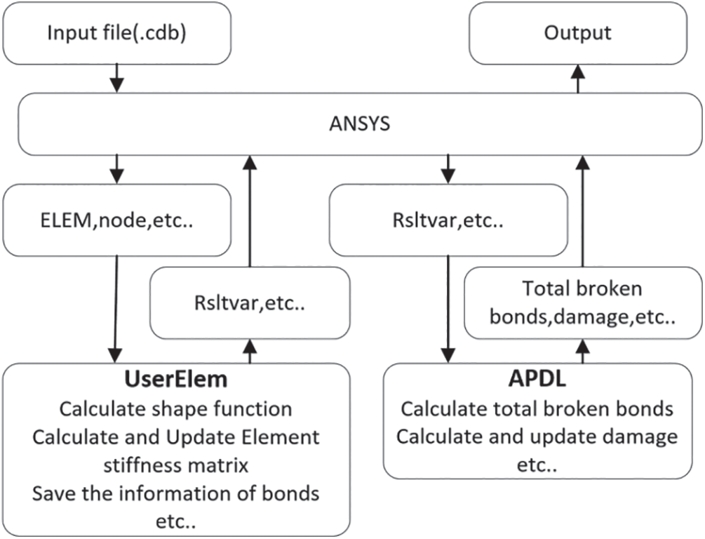
Figure 5: Implementation details of PeriFEM in ANSYS using APDL and UserElem

In addition, we also need both peridynamic elements and local elements in ANSYS, as stated in the previous subsection. The only difference is in how the damage information is obtained. The process of visualization in ANSYS can be summarized as follows. First, the broken-bond information (Rsltvar) is obtained via the UserElem subroutine. Then, RsltVar is extracted from UserElem by APDL, based on which the damage information for each local element can be calculated according to Eq. (7). Finally, the damage contour can be displayed in the postprocess module of ANSYS via the local elements.

Remark 4.Even though PeriFEM allows both continuous and discrete local elements [31], only continuous local elements are available in ABAQUS and ANSYS. Thus, only continuous local elements were used in the present study.

6  Numerical Examples

6.1 2D Tests for the Verification and Comparison of ANSYS and ABAQUS

The purpose of the tests presented in this subsection is twofold. On the one hand, we first wish to verify the correct functioning of the code for implementing PeriFEM in ANSYS and ABAQUS. On the other hand, as different convergence criteria were adopted in ANSYS and ABAQUS, the convergence performance, computational cost, and predicted crack patterns need to be compared between ANSYS and ABAQUS. To this end, 2D benchmark examples are carried out using both ANSYS and ABAQUS.

6.1.1 Single-Edge-Notched Plate under Tension

First, we consider a tension test for a single-edge-notched plate. The geometry and boundary conditions are shown in Fig. 6. Young’s modulus is set to E=200 GPa, Poisson’s ratio is ν=1/3, and the critical stretch is scrit=0.02. The plate is discretized with quadrilateral local elements and the mesh size is h=5 mm. The horizon is chosen as δ=3h and 9860 peridynamic elements are generated. The boundary conditions are divided into 100 incremental steps.

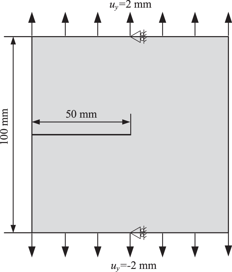
Figure 6: Geometry and boundary conditions of a single-edge-notched plate

It is known that the crack will initiate from the notch tip and propagate horizontally to the right for this test. As shown in Fig. 7, the effective damage contours, which reveal the crack, predicted by ANSYS and ABAQUS are correct. This verifies the correct integration of the PeriFEM code into ANSYS and ABAQUS. Moreover, Fig. 8a shows the iteration numbers in each incremental step of both ANSYS and ABAQUS. It can be seen that the iteration numbers almost coincided with each other in this test, even though different convergence criteria are adopted. Fig. 8b displays the total computational costs of both ANSYS and ABAQUS. In this example, the total number of iterations of ANSYS and ABAQUS is similar, but the overall CPU times are considerably different. Notably, several factors may affect the overall CPU time. For instance, the way in which post-processing is implemented may have had a considerable impact. In ABAQUS, post-processing is implemented through the UMAT subroutine, whereas it is implemented through in-house APDL code in ANSYS.

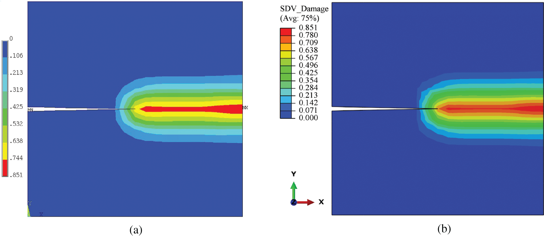
Figure 7: Contours of the effective damage for a single-edge-notched plate computed by (a) ANSYS and (b) ABAQUS

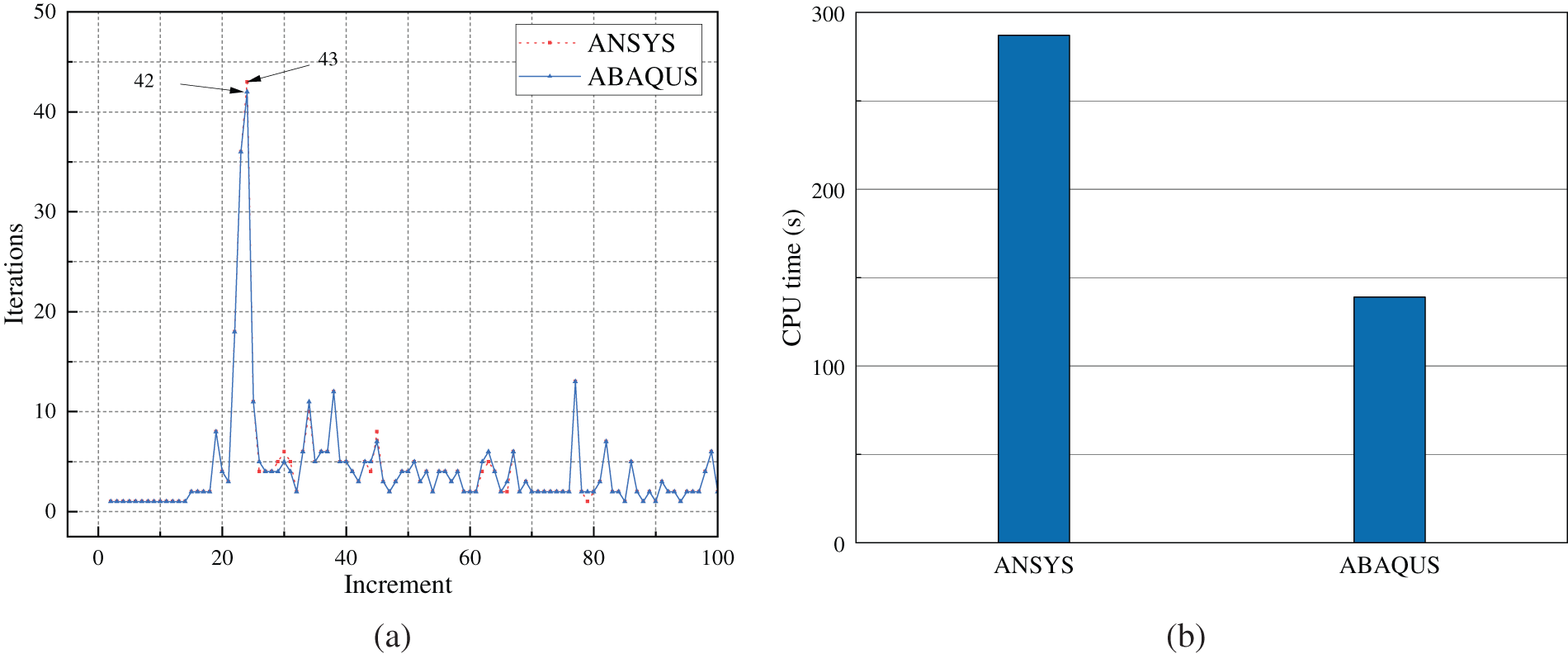
Figure 8: Comparison of the number of iterations in each incremental step and total CPU time between ANSYS and ABAQUS

6.1.2 L-Shaped Panel

We now consider the case of an L-shaped panel. The geometry and boundary conditions are shown in Fig. 9. Young’s modulus is set to E=25.85 GPa, Poisson’s ratio is ν=1/3, and the critical stretch is scrit=0.0006. The panel is discretized with quadrilateral local elements, and the mesh size is h≈3.6 mm. The horizon is chosen as δ=3h and 909262 peridynamic elements are generated. The boundary conditions are divided into 140 incremental steps.

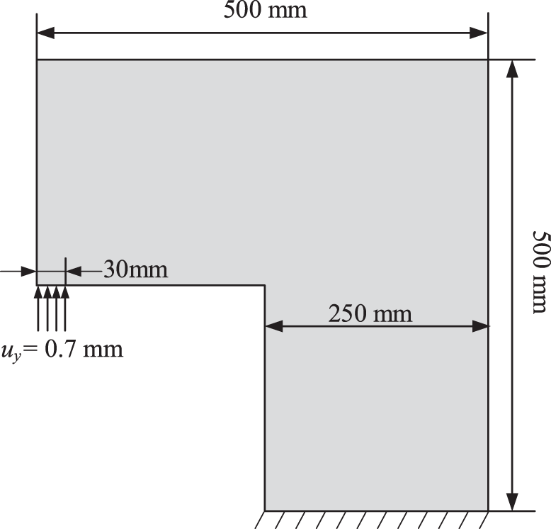
Figure 9: Geometry and boundary conditions of an L-shaped panel

Figs. 10a and 10b display the effective damage zones predicted by ANSYS and ABAQUS, respectively, and Fig. 10c compares the predicted crack paths with the experimental failure zone reported in [43]. The simulated results obtained using both ANSYS and ABAQUS are in good agreement with the experimental data, which further verifies the developed code. Moreover, Fig. 11 shows the number of iterations in each incremental step for ANSYS and ABAQUS. The similarity between the two curves indicates that the simulated results by ANSYS and ABAQUS are in line with each other.

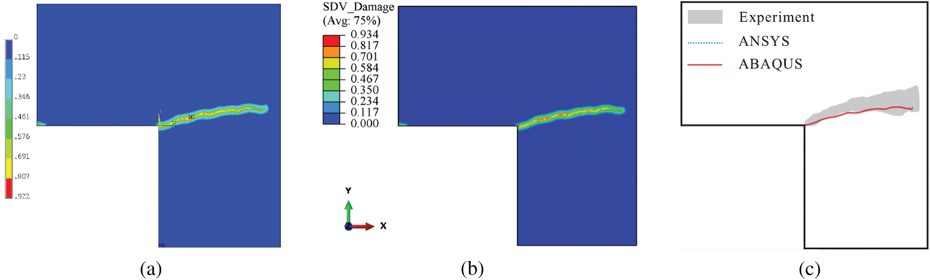
Figure 10: Contours of the effective damage for an L-shaped panel computed by (a) ANSYS and (b) ABAQUS, as well as (c) a comparison with experimental results

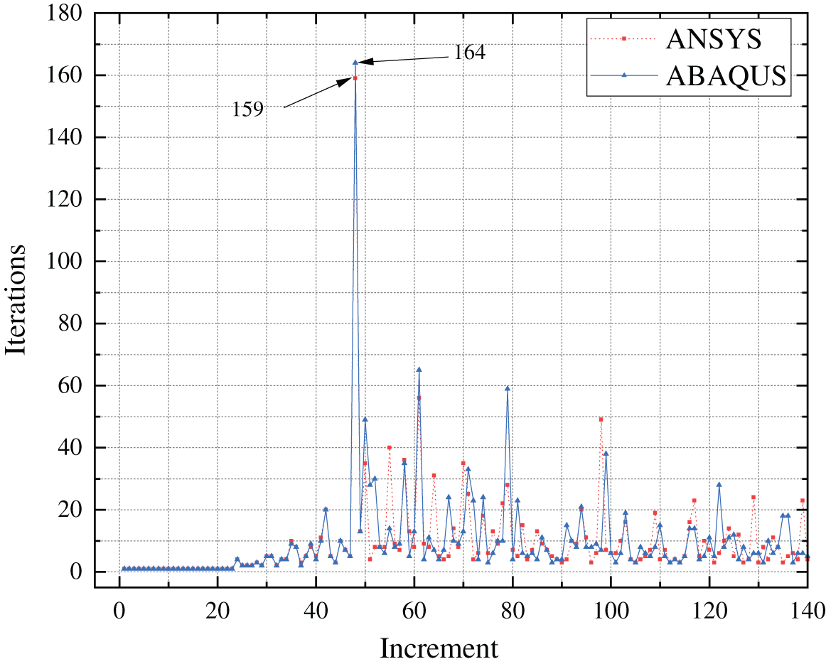
Figure 11: Comparison of the number of iterations in each incremental step between ANSYS and ABAQUS

6.1.3 Double-Edge-Notched Plate under Tension and Shear

In this test, we investigate the mixed-mode fracture of a double-edge-notched plate. The geometry and boundary conditions are shown in Fig. 12. Young’s modulus is set to E=30 GPa, Poisson’s ratio is ν=1/3, and the critical stretch is scrit=0.02. The plate is discretized with quadrilateral local elements, and the mesh size is h ≈1.25 mm. The horizon is set as δ=3h, and 1019120 peridynamic elements are generated. The boundary conditions are divided into 80 incremental steps.

Figure 12: Geometry and boundary condition of a double-edge-notched plate

The predicted effective damage contours and a comparison with the experimental results reported in [44] are shown in Fig. 13. It can be seen that the predicted crack paths are in good agreement with the experimental results. However, one may note that the simulated results obtained with ABAQUS presented in the figure are only up to the 20th incremental step, but not for the 80th incremental step. This is because from the 21st increment onward, ABAQUS encounters a convergence issue, as shown in Fig. 14. Figs. 14a and 14b display the number of broken bonds and the largest residual force during the iteration, respectively. Although the number of broken bonds no longer increases, the largest residual force still does not satisfy the convergence condition and falls into a regular oscillation, which means that the iteration will never converge.

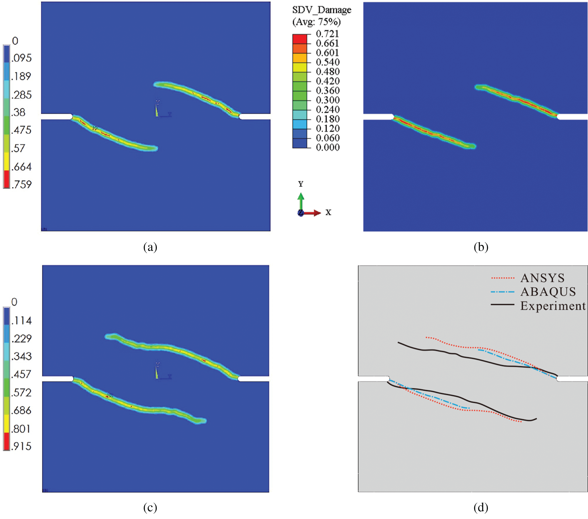
Figure 13: Contours of the effective damage for a double-edged plate obtained with (a) ANSYS at 20th incremental step, (b) ABAQUS at 20th incremental step, and (c) ANSYS at 80th incremental step, as well as (d) a comparison with experimental results

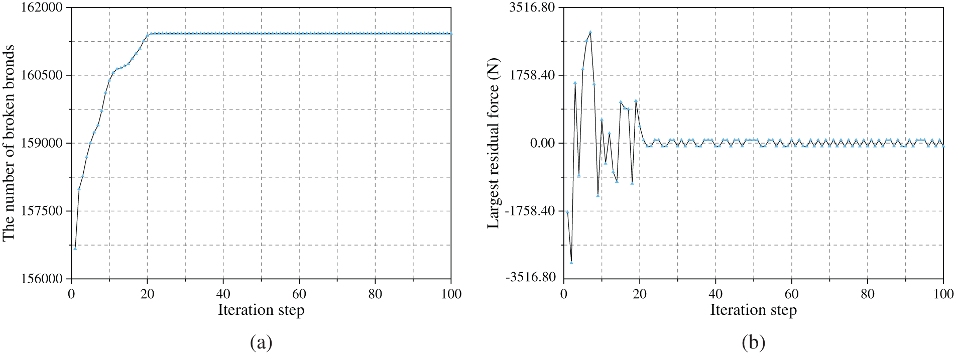
Figure 14: Iteration information of ABAQUS at the 21st incremental step: (a) number of broken bonds and (b) largest residual force

Remark 5. The above non-convergence phenomenon is not a problem of the code but may stem from the constitutive model and the specimen. It was reported in [45] that the discontinuity of the constitutive model can result in convergence issues.

6.2 3D Tests

We now investigate 3D examples using ANSYS and ABAQUS to verify the ability of the proposed method to deal with complex problems. In all tests, hexahedral local elements are used.

6.2.1 Three-Point Bending Test on a Slanted Notched Beam

This example shows a three-point bending test of a beam with a slanted notch. More specifically, the vertical notch had an inclination of θ=45∘ with respect to the longitudinal mid-plane section of the beam. We consider the same geometry and boundary conditions as those reported in [46], which are presented in Fig. 15.

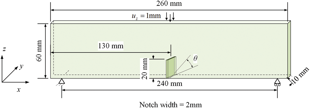
Figure 15: Geometry and boundary condition for the slanted notched beam

Young’s modulus is set to E=2.8 GPa, Poisson’s ratio is ν=1/4, and the critical stretch is scrit=0.00235. The beam is discretized with hexahedral local elements and the mesh size is h≈2.0 mm. The horizon is set as δ=3h, and 1618634 peridynamic elements are generated. The prescribed displacement is equally divided into 100 incremental steps.

The ABAQUS software is used for this test. The predicted effective damage contours are shown in Fig. 16. Initially, a mode III fracture is predominant. Therefore, it can be seen that the crack face first propagates along the direction of the slanted notch, which stems from the stress concentration around the notch caused by the asymmetrical bending of the beam. Then, as the crack propagated, the mid-plane section acts as an attractor of the crack surface owing to the coincidence between the loading and itself. Thus, a mode I fracture gradually became predominant. It can be seen that the crack surface twists gradually in space as the prescribed displacement increased. Finally, it aligns with the mid-plane section. We can conclude that the torsion of the crack surface was successfully captured in the simulation, although this torsion was not very obvious. This is due to a limitation in computational resources; the mesh is not sufficiently fine. Nonetheless, the overall results show that the proposed technique can be successfully applied to 3D problems.

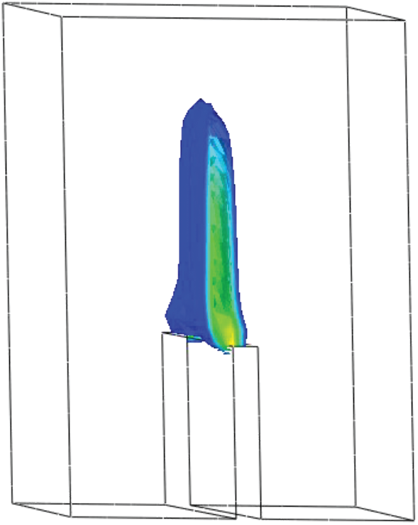
Figure 16: Crack pattern and damage profile for the slanted notched beam

To better display the results, prospective views of the damage profile at various heights above the notch are shown in Fig. 17. We used two reference (white) lines; one for marking the main damage zone and the other for marking the direction of the slanted notch to better show the rotation angle of the main damage zone. The difference between the revolving angles at different heights reveals the rotation of the damage field. The damage starts from the slanted notch, and then twists spatially and develops along the vertical direction. First, the damage field revolving angle increased rapidly. Then, it increases slowly. Finally, the top view of the damage profile is nearly along the mid-plane section of the geometric model.

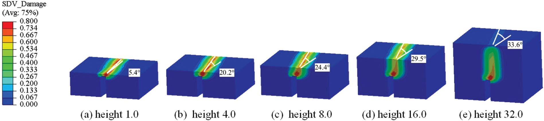
Figure 17: Predicted damage profiles at different heights above the notch

6.2.2 Prismatic Skew-Notched Beam under Torsion

Finally, a prismatic skew-notched concrete beam under torsion is simulated using ANSYS. This example was also tested by Brokenshire [47] and reported in detail in [48]. The concrete specimen used in those experiments included two steel frames at both ends. However, due to Saint Venant’s principle, these steel frames can be simplified as displacement constraints and have minimal influence on the stress state near the notch. The geometry and boundary conditions of such a simplified model are shown in Fig. 18.

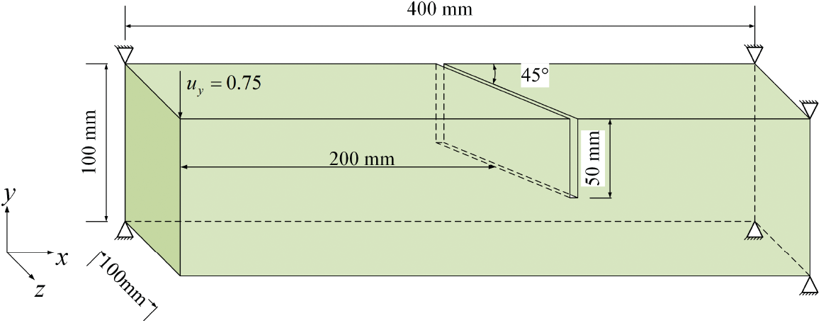
Figure 18: Geometry and boundary conditions of the prismatic skew-notched beam

Young’s modulus is set to E=35 GPa, Poisson’s ratio is ν=1/4, and the critical stretch is scrit=0.0006316. The beam is discretized with hexahedral local elements and the mesh size is h≈5 mm. The horizon is set as δ=3h and 3886626 peridynamic elements are generated. The prescribed displacement is equally divided into 50 incremental steps.

Fig. 19 shows the displacement contour and three different views of the damage iso-surface at the last incremental step. Fig. 19a shows the displacement contour of the beam, and Figs. 19b–19d show top, slanted, and side views of the damage isosurface, respectively. A skew-symmetrical crack surface with a complex twisting pattern can be clearly observed from these three different views. Moreover, distinct antisymmetric crack kinking can be observed along the straight crack front of the inclined initial crack. This is caused by the combination of the mode I and mode III loading conditions. Meanwhile, from Fig. 19c, we can observe that crack kinking becomes more pronounced further away from the notch. This is because when the crack initiates, mode I fracture is predominant. However, as the crack propagates, mode III fracture plays a more important role, which in turn causes crack kinking to become more pronounced.

Figure 19: (a) Displacement contour and (b) top view, (c) slanted view, and (d) side view of the damage isosurface of the concrete beam at the last incremental step

Fig. 20 shows three top views of the damage isosurface obtained using three different methods. Fig. 20a shows the results obtained by ANSYS using PeriFEM, Fig. 20b shows the results obtained from an experiment on PMMA [49], and Fig. 20c shows the results obtained by ABAQUS using the phase-field method [46]. The crack surface shown in Fig. 20a is similar to those in Figs. 20b and 20c. Moreover, the above results are consistent with those obtained from an isotropic damage model in the context of stabilized mixed finite elements [50], which demonstrates the feasibility of using PeriFEM in ANSYS to simulate 3D problems. Note that the maximum vertical displacement in ANSYS is 0.75 mm, which is half the 1.5 mm value used in the experimental test and ABAQUS simulation. According to the load–displacement curve in [46], the beam completely fractures when the vertical displacement is 0.75 mm.

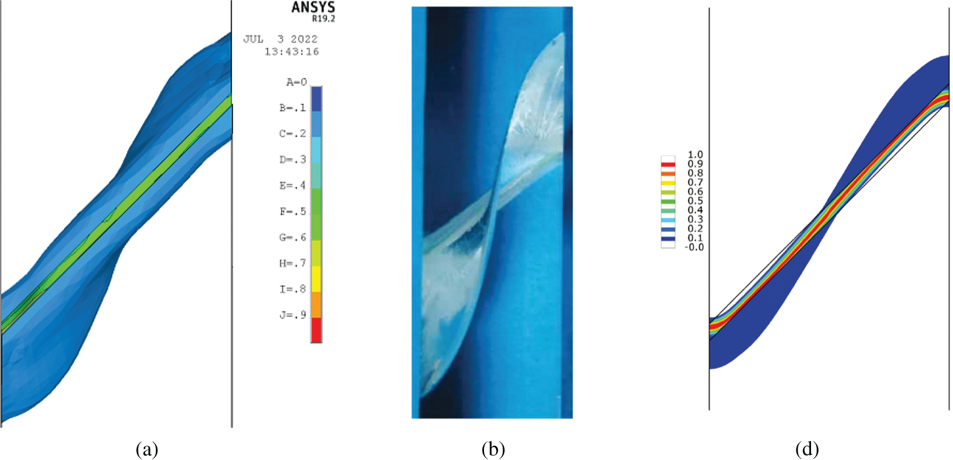
Figure 20: Top view of the damage surface obtained using different methods: (a) ANSYS with PeriFEM; (b) PMMA test in [49]; (c) ABAQUS and the phase-field method [46]

7  Conclusions

In this study, we proposed a unified implementation strategy for peridynamics in commercial FEM software by leveraging available APIs and using the peridynamics-based finite element method. As a demonstration of this strategy, PeriFEM was implemented in ANSYS using UPFs and ABAQUS using UEL. Various 2D and 3D numerical tests demonstrated the effectiveness of the proposed strategy for brittle fracture modeling. Based on the proposed implementation details and the simulation results obtained in this study, we can conclude the following:

•   It is convenient to integrate PeriFEM into commercial FEM software through its API via the proposed unified implementation strategy.

•   The brittle fracture of materials under complex loads can be simulated by the proposed strategy using commercial FEM software.

Therefore, the present work facilitates the application of peridynamics in engineering practice. Future work will focus on implementing coupled local/non-local models in software to improve computational efficiency and reduce boundary effects.

Funding Statement: The authors gratefully acknowledge the financial support received from the National Natural Science Foundation of China (12272082, 11872016) and the National Key Laboratory of Shock Wave and Detonation Physics (JCKYS2021212003).

Conflicts of Interest: The authors declare that they have no conflicts of interest to report regarding the present study.

1Although it is unknown for a given element, this does not matter as we only need the total external force vector after assembling the whole structure.

References

1. Hey, A. J., Tansley, S., Tolle, K. M. (2009). The fourth paradigm: Data-intensive scientific discovery, vol. 1. WA: Microsoft Research Redmond. [Google Scholar]

2. Logan, D. L. (2016). A first course in the finite element method. Boston MA, USA: Cengage Learning. [Google Scholar]

3. Belytschko, T., Liu, W. K., Moran, B., Elkhodary, K. (2014). Nonlinear finite elements for continua and structures. West Sussex, UK: John Wiley & Sons. [Google Scholar]

4. Fang, X. J., Jin, F. (2007). Extended finite element method based on ABAQUS. Engineering Mechanics, 24(7), 6–10. [Google Scholar]

5. Li, W., Nguyen-Thanh, N., Zhou, K. (2020). Phase-field modeling of brittle fracture in a 3D polycrystalline material via an adaptive isogeometric-meshfree approach. International Journal for Numerical Methods in Engineering, 121(22), 5042–5065. https://doi.org/10.1002/nme.6509 [Google Scholar] [CrossRef]

6. Nguyen-Thanh, N., Li, W., Huang, J., Zhou, K. (2020). Adaptive higher-order phase-field modeling of anisotropic brittle fracture in 3D polycrystalline materials. Computer Methods in Applied Mechanics and Engineering, 372(2), 113434. https://doi.org/10.1016/j.cma.2020.113434 [Google Scholar] [CrossRef]

7. Lindgaard, E., Bak, B., Glud, J., Sjølund, J., Christensen, E. (2017). A user programmed cohesive zone finite element for ANSYS Mechanical. Engineering Fracture Mechanics, 180(2), 229–239. https://doi.org/10.1016/j.engfracmech.2017.05.026 [Google Scholar] [CrossRef]

8. Msekh, M. A., Sargado, J. M., Jamshidian, M., Areias, P. M., Rabczuk, T. (2015). Abaqus implementation of phase-field model for brittle fracture. Computational Materials Science, 96(8), 472–484. https://doi.org/10.1016/j.commatsci.2014.05.071 [Google Scholar] [CrossRef]

9. Molnár, G., Gravouil, A. (2017). 2D and 3D Abaqus implementation of a robust staggered phase-field solution for modeling brittle fracture. Finite Elements in Analysis and Design, 130(582–593), 27–38. https://doi.org/10.1016/j.finel.2017.03.002 [Google Scholar] [CrossRef]

10. Wu, J. Y., Huang, Y. (2020). Comprehensive implementations of phase-field damage models in Abaqus. Theoretical and Applied Fracture Mechanics, 106(4), 102440. https://doi.org/10.1016/j.tafmec.2019.102440 [Google Scholar] [CrossRef]

11. Silling, S. A. (2000). Reformulation of elasticity theory for discontinuities and long-range forces. Journal of the Mechanics and Physics of Solids, 48(1), 175–209. https://doi.org/10.1016/S0022-5096(99)00029-0 [Google Scholar] [CrossRef]

12. Silling, S. A., Epton, M., Weckner, O., Xu, J., Askari, E. (2007). Peridynamic states and constitutive modeling. Journal of Elasticity, 88(2), 151–184. https://doi.org/10.1007/s10659-007-9125-1 [Google Scholar] [CrossRef]

13. Li, J., Li, S., Lai, X., Liu, L. (2022). Peridynamic stress is the static first Piola–Kirchhoff virial stress. International Journal of Solids and Structures, 241(1–2), 111478. https://doi.org/10.1016/j.ijsolstr.2022.111478 [Google Scholar] [CrossRef]

14. Zhang, N., Gu, Q., Huang, S., Xue, X., Li, S. (2021). A practical bond-based peridynamic modeling of reinforced concrete structures. Engineering Structures, 244(1), 112748. https://doi.org/10.1016/j.engstruct.2021.112748 [Google Scholar] [CrossRef]

15. Chen, Z., Chu, X. (2021). Peridynamic modeling and simulation of fracture process in fiber-reinforced concrete. Computer Modeling in Engineering & Sciences, 127(1), 241–272. https://doi.org/10.32604/cmes.2021.015120 [Google Scholar] [CrossRef]

16. Han, J., Li, S., Yu, H., Li, J., Zhang, A. M. (2022). On nonlocal cohesive continuum mechanics and cohesive peridynamic modeling (CPDM) of inelastic fracture. Journal of the Mechanics and Physics of Solids, 164, 104894. https://doi.org/10.1016/j.jmps.2022.104894 [Google Scholar] [CrossRef]

17. Chen, X., Gunzburger, M. (2011). Continuous and discontinuous finite element methods for a peridynamics model of mechanics. Computer Methods in Applied Mechanics and Engineering, 200(9–12), 1237–1250. https://doi.org/10.1016/j.cma.2010.10.014 [Google Scholar] [CrossRef]

18. Azdoud, Y., Han, F., Lubineau, G. (2014). The morphing method as a flexible tool for adaptive local/non-local simulation of static fracture. Computational Mechanics, 54(3), 711–722. https://doi.org/10.1007/s00466-014-1023-3 [Google Scholar] [CrossRef]

19. Ren, B., Wu, C., Askari, E. (2017). A 3D discontinuous Galerkin finite element method with the bond-based peridynamics model for dynamic brittle failure analysis. International Journal of Impact Engineering, 99(5), 14–25. https://doi.org/10.1016/j.ijimpeng.2016.09.003 [Google Scholar] [CrossRef]

20. Silling, S. A. (2003). Dynamic fracture modeling with a meshfree peridynamic code. In: Computational fluid and solid mechanics 2003, pp. 641–644. Massachusetts, USA: Elsevier. [Google Scholar]

21. Silling, S. A., Askari, E. (2005). A meshfree method based on the peridynamic model of solid mechanics. Computers & Structures, 83(17–18), 1526–1535. https://doi.org/10.1016/j.compstruc.2004.11.026 [Google Scholar] [CrossRef]

22. Seleson, P., Littlewood, D. J. (2016). Convergence studies in meshfree peridynamic simulations. Computers & Mathematics with Applications, 71(11), 2432–2448. https://doi.org/10.1016/j.camwa.2015.12.021 [Google Scholar] [CrossRef]

23. Diyaroglu, C., Madenci, E., Phan, N. (2019). Peridynamic homogenization of microstructures with orthotropic constituents in a finite element framework. Composite Structures, 227, 111334. https://doi.org/10.1016/j.compstruct.2019.111334 [Google Scholar] [CrossRef]

24. Huang, X., Bie, Z., Wang, L., Jin, Y., Liu, X. et al. (2019). Finite element method of bond-based peridynamics and its ABAQUS implementation. Engineering Fracture Mechanics, 206(1), 408–426. https://doi.org/10.1016/j.engfracmech.2018.11.048 [Google Scholar] [CrossRef]

25. Bie, Y., Liu, Z., Yang, H., Cui, X. (2020). Abaqus implementation of dual peridynamics for brittle fracture. Computer Methods in Applied Mechanics and Engineering, 372, 113398. https://doi.org/10.1016/j.cma.2020.113398 [Google Scholar] [CrossRef]

26. Anicode, S. V. K., Madenci, E. (2022). Bond-and state-based peridynamic analysis in a commercial finite element framework with native elements. Computer Methods in Applied Mechanics and Engineering, 398(12), 115208. https://doi.org/10.1016/j.cma.2022.115208 [Google Scholar] [CrossRef]

27. Macek, R. W., Silling, S. A. (2007). Peridynamics via finite element analysis. Finite Elements in Analysis and Design, 43(15), 1169–1178. https://doi.org/10.1016/j.finel.2007.08.012 [Google Scholar] [CrossRef]

28. Ren, B., Wu, C., Seleson, P., Zeng, D., Nishi, M. et al. (2022). An FEM-based peridynamic model for failure analysis of unidirectional fiber-reinforced laminates. Journal of Peridynamics and Nonlocal Modeling, 4(1), 139–158. https://doi.org/10.1007/s42102-021-00063-0 [Google Scholar] [CrossRef]

29. https://www.lstc-cmmg.org/peri-dynamics [Google Scholar]

30. Han, F., Li, Z. (2022). A peridynamics-based finite element method (PeriFEM) for quasi-static fracture analysis. Acta Mechanica Solida Sinica, 35(3), 446–460. https://doi.org/10.1007/s10338-021-00307-y [Google Scholar] [CrossRef]

31. Li, Z., Han, F. (2023). The peridynamics-based finite element method (PeriFEM) with adaptive continuous/discrete element implementation for fracture simulation. Engineering Analysis with Boundary Elements, 146(5), 56–65. https://doi.org/10.1016/j.enganabound.2022.09.033 [Google Scholar] [CrossRef]

32. Han, F., Li, Z., Zhang, J., Liu, Z., Yao, C. et al. (2022). ABAQUS and ANSYS implementations of peridynamics-based finite element method (PeriFEM) for brittle fracture. https://www.researchsquare.com/article/rs-1888499/v1.pdf [Google Scholar]

33. Madenci, E., Oterkus, E. (2014). Peridynamic theory and its applications. New York, NY: Springer. [Google Scholar]

34. Bobaru, F., Yang, M., Alves, L. F., Silling, S. A., Askari, E. et al. (2009). Convergence, adaptive refinement, and scaling in 1D peridynamics. International Journal for Numerical Methods in Engineering, 77(6), 852–877. https://doi.org/10.1002/nme.2439 [Google Scholar] [CrossRef]

35. Lubineau, G., Azdoud, Y., Han, F., Rey, C., Askari, A. (2012). A morphing strategy to couple non-local to local continuum mechanics. Journal of the Mechanics and Physics of Solids, 60(6), 1088–1102. https://doi.org/10.1016/j.jmps.2012.02.009 [Google Scholar] [CrossRef]

36. Wang, Y., Han, F., Lubineau, G. (2021). Strength-induced peridynamic modeling and simulation of fractures in brittle materials. Computer Methods in Applied Mechanics and Engineering, 374(1), 113558. https://doi.org/10.1016/j.cma.2020.113558 [Google Scholar] [CrossRef]

37. Yu, H., Li, S. (2020). On energy release rates in peridynamics. Journal of the Mechanics and Physics of Solids, 142(3), 104024. https://doi.org/10.1016/j.jmps.2020.104024 [Google Scholar] [CrossRef]

38. Han, F., Lubineau, G., Azdoud, Y., Askari, A. (2016). A morphing approach to couple state-based peridynamics with classical continuum mechanics. Computer Methods in Applied Mechanics and Engineering, 301, 336–358. https://doi.org/10.1016/j.cma.2015.12.024 [Google Scholar] [CrossRef]

39. Ren, H., Zhuang, X., Cai, Y., Rabczuk, T. (2016). Dual-horizon peridynamics. International Journal for Numerical Methods in Engineering, 108(12), 1451–1476. https://doi.org/10.1002/nme.5257 [Google Scholar] [CrossRef]

40. Pasetto, M., Shen, Z., D’Elia, M., Tian, X., Trask, N. et al. (2022). Efficient optimization-based quadrature for variational discretization of nonlocal problems. Computer Methods in Applied Mechanics and Engineering, 396(6), 115104. https://doi.org/10.1016/j.cma.2022.115104 [Google Scholar] [CrossRef]

41. Morales, R. C., Baek, J., Sharp, D., Aderounmu, A., Wei, H. et al. (2022). Mode-II fracture response of pmma under dynamic loading conditions. Journal of Dynamic Behavior of Materials, 8(1), 104–121. https://doi.org/10.1007/s40870-021-00320-9 [Google Scholar] [CrossRef]

42. Dassault Systëmes (2012). Abaqus analysis user’s manual.http://130.149.89.49:2080/v6.12/books/usb/ default.htm [Google Scholar]

43. Winkler, B. J. (2001). Traglastuntersuchungen von unbewehrten und bewehrten Betonstrukturen auf der Grundlage eines objektiven Werkstoffgesetzes für Beton (Ph.D. Thesis). Universität Innsbruck. [Google Scholar]

44. Nooru-Mohamed, M., Schlangen, E., van Mier, J. G. (1993). Experimental and numerical study on the behavior of concrete subjected to biaxial tension and shear. Advanced Cement Based Materials, 1(1), 22–37. https://doi.org/10.1016/1065-7355(93)90005-9 [Google Scholar] [CrossRef]

45. Ni, T., Zaccariotto, M., Zhu, Q. Z., Galvanetto, U. (2019). Static solution of crack propagation problems in peridynamics. Computer Methods in Applied Mechanics and Engineering, 346(3), 126–151. https://doi.org/10.1016/j.cma.2018.11.028 [Google Scholar] [CrossRef]

46. Wu, J. Y., Huang, Y., Zhou, H., Nguyen, V. P. (2021). Three-dimensional phase-field modeling of mode I+II/III failure in solids. Computer Methods in Applied Mechanics and Engineering, 373(48), 113537. https://doi.org/10.1016/j.cma.2020.113537 [Google Scholar] [CrossRef]

47. Brokenshire, D. (1996). A study of torsion fracture test (Ph.D. Thesis). Cardiff University. [Google Scholar]

48. Jefferson, A. D., Barr, B., Bennett, T., Hee, S. (2004). Three dimensional finite element simulations of fracture tests using the craft concrete model. Computers and Concrete, 1(3), 261–284. https://doi.org/10.12989/cac.2004.1.3.261 [Google Scholar] [CrossRef]

49. Buchholz F. G., Just V., Richard, H. (2005). Computational simulation and experimental findings of three-dimensional fatigue crack growth in a single-edge notched specimen under torsion loading. Fatigue & Fracture of Engineering Materials & Structures, 28(1–2), 127–134. https://doi.org/10.1111/j.1460-2695.2005.00864.x [Google Scholar] [CrossRef]

50. Benedetti, L., Cervera, M., Chiumenti, M. (2017). 3D numerical modelling of twisting cracks under bending and torsion of skew notched beams. Engineering Fracture Mechanics, 176(3), 235–256. https://doi.org/10.1016/j.engfracmech.2017.03.025 [Google Scholar] [CrossRef]

51. Azdoud, Y., Han, F., Lubineau, G. (2013). A morphing framework to couple non-local and local anisotropic continua. International Journal of Solids and Structures, 50(9), 1332–1341. https://doi.org/10.1016/j.ijsolstr.2013.01.016 [Google Scholar] [CrossRef]

Appendix

Appendix A. Calculation of c~(θ,φ) for anisotropic materials

In 2013, Azdoud et al. [51] derived an expression for c(ξ) using the real spherical harmonic expansion technique, where c~(θ,φ) in Eq. (4) was defined as

c~(θ,φ)=a00+∑k=1+∞[∑m=0kPkm(cos⁡(θ))(akmcos⁡(mφ)+bkmsin⁡(mφ))].(32)

Here, θ and φ supplemented with ‖ξ‖ comprise the spherical coordinates of bond ξ, as shown in Fig. 21. a00, akm, and bkm are real parameters and Pkm are Legendre functions. They showed that, for the orthotropic model, it holds that

c~(θ,φ)=a00+a20P20(cos⁡(θ))+a22cos⁡(2ϕ)P22(cos⁡(θ))+a40P40(cos⁡(θ))+a42cos⁡(2ϕ)P42(cos⁡(θ))+a44cos⁡(4ϕ)P44(cos⁡(θ)),(33)

whereas for the transverse isotropic model (assuming that e3 is the reference direction of an axisymmetric material), it holds that

c~(θ,φ)=c~(θ)=a0+a2P20(cos⁡θ)+a4P40(cos⁡θ).(34)

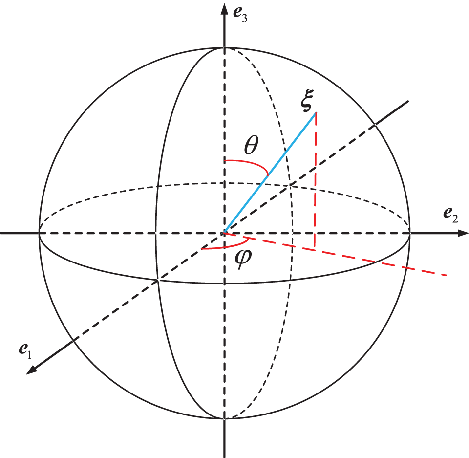
Figure 21: Spherical coordinates for bond ξ

In addition, they gave an expression of the real parameters in Eqs. (33) and (34) for c^(‖ξ‖)=1. However, they did not explain how to calculate these real parameters; thus, it is still difficult to determine the real parameters for c^(‖ξ‖)≠1.

The parameters in Eqs. (33) and (34) can be determined according to the deformation energy equivalence; the key point is to define an equivalent stiffness tensor. Based on the assumption of uniform strain fields, Lubineau et al. derived an effective stiffness tensor in [35] as

D=∫Hδ(x)c(ξ)2ξ⊗ξ⊗ξ⊗ξdVx′.(35)

Let us denote the classical stiffness tensor by E and set

D=E.(36)

Then, we can determine the parameters.

Appendix B. Orthotropic model

In the classical orthotropic model, there are nine independent variables in E, which are

E1111,E2222,E3333,E1122,E1133,E2233,E1212,E1313,E2323.(37)

In the peridynamic orthotropic model, there are only six independent variables in D because of the centrosymmetry of the long-range force. These variables are

D1111,D2222,D3333,D1122=D1212,D1133=D1313,D2233=D2323.(38)

Therefore, Eq. (36) implies that

D1111=E1111,D2222=E2222,D3333=E3333,D1122=E1122,D1133=E1133,D2233=E2233.(39)

Substituting Eq. (33) into Eq. (35), we have

D=a00D00+a20D20+a22D22+a40D40+a42D42+a44D44,(40)

where

Dij=∫Hδ(x)c1(‖ξ‖)cos(jφ)Pij(cos(θ))2ξ⊗ξ⊗ξ⊗ξdVx′,i,j=0,2,4 and j≤i.(41)

Then, Eq. (39) implies that

[D111100D111120D111122D111140D111142D111144D222200D222220D222222D222240D222242D222244D333300D333320D333322D333340D333342D333344D112200D112220D112222D112240D112242D112244D113300D113320D113322D113340D113342D113344D223300D223320D223322D223340D223342D223344][a00a20a22a40a42a44]=[E1111E2222E3333E1122E1133E2233].(42)

By solving the above equations, the parameters in Eq. (33) can be obtained.

Appendix C. Transverse isotropic model

In the classical transverse isotropic model, there are five independent variables in E (assuming that e3 is the reference direction of an axisymmetric material). These variables are

E1111,E3333,E1122,E1133,E1313.(43)

In the peridynamic transverse isotropic model, there are only three independent variables in D because of the centrosymmetry of the long-range force. These variables are

D1111,D3333,D1133=D1313,(44)

and D1122 depends on the other coefficients. Therefore, Eq. (36) implies that

D1111=E1111,D3333=E3333,D1133=E1133.(45)

Substituting Eq. (34) into Eq. (35), we have

D=a0D0+a2D2+a4D4,(46)

where

Di=∫Hδ(x)c1(‖ξ‖)Pi0(cos(θ))2ξ⊗ξ⊗ξ⊗ξdVx′,i=0,2,4.(47)

Then, Eq. (45) implies that

[D11110D11112D11114D33330D33332D33334D11330D11332D11334][a0a2a4]=[E1111E3333E1133].(48)

By solving the above equations, the parameters in Eq. (34) can be obtained.