
 Submit a Paper
 Propose a Special lssue
 Open Access
ARTICLE

STPGTN–A Multi-Branch Parameters Identification Method Considering Spatial Constraints and Transient Measurement Data
Jiangsu Key Laboratory of Big Data Analysis Technology, Nanjing University of Information Science and Technology, Nanjing, 210044, China
* Corresponding Author: Liguo Weng. Email:
(This article belongs to the Special Issue: Machine Learning-Guided Intelligent Modeling with Its Industrial Applications)
Computer Modeling in Engineering & Sciences 2023, 136(3), 2635-2654. https://doi.org/10.32604/cmes.2023.025405
Received 09 July 2022; Accepted 15 November 2022; Issue published 09 March 2023
 View Full Text
 Download PDF
Abstract
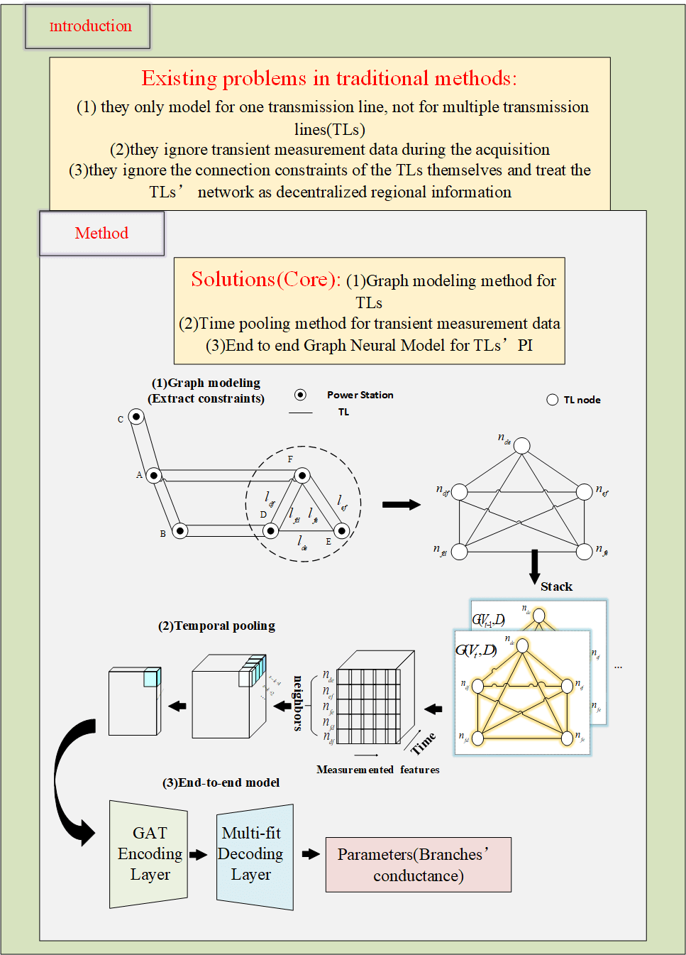
Transmission line (TL) Parameter Identification (PI) method plays an essential role in the transmission system. The existing PI methods usually have two limitations: (1) These methods only model for single TL, and can not consider the topology connection of multiple branches for simultaneous identification. (2) Transient bad data is ignored by methods, and the random selection of terminal section data may cause the distortion of PI and have serious consequences. Therefore, a multi-task PI model considering multiple TLs’ spatial constraints and massive electrical section data is proposed in this paper. The Graph Attention Network module is used to draw a single TL into a node and calculate its influence coefficient in the transmission network. Multi-Task strategy of Hard Parameter Sharing is used to identify the conductance of multiple branches simultaneously. Experiments show that the method has good accuracy and robustness. Due to the consideration of spatial constraints, the method can also obtain more accurate conductance values under different training and testing conditions.Graphic Abstract
Keywords
With the increasing energy demand, the power transmission network is becoming more and more complex, and the stability requirements of the distribution system are getting higher and higher. Transmission line parameter identification method plays an essential role in the smooth operation of power distribution system. However, due to changes in temperature and humidity and sag caused by line aging, line parameters will change inevitably [1]. For that reason, the parameters must be regularly updated. Therefore, it is important to discuss a real-time PI method with high accuracy and strong robustness.
Currently, the main methods of PI include theoretical calculation, off-line manual measurement and real-time measurement based on measured data. Compared with high-cost manual off-line measurement or formula calculation with low confidence, PI based on measured data has attracted great attention because of its convenience and economy. According to the data source, these methods can be divided into two categories: (1) parameter identification based on SCADA (Supervisory Control And Data Acquisition) System [2–4]. (2) Parameter identification based on PMU (Power Management Unit) System [5–7]. Although the voltage and current information obtained by PMU is more comprehensive and accurate than SCADA’s, the PMU devices still have the problem of phase angle synchronization [8]. Besides, due to the high cost of PMU devices, it may not be economically viable to install PMU on each TL of the power system. Therefore, this paper will focus on the common SCADA data.
However, the existing traditional identification methods based on SCADA data have limitations on two levels as follows:
On one hand, traditional method considers the cross-section data of SCADA too ideally. First of all, the Remote Terminal Unit (RTU) of current transmission system adopts the t-polling mechanism at a given time to collect data [9]. It stores the data of multiple acquisition terminals as section data in the database, and generally takes seconds as the section time scale, which will generate a large amount of historical data. The data section used by traditional PI methods is selected by manual experience. It is easy to select the section where the system has abnormalities and noise interference, causing the failure of generating effective branch parameters [10]. At the same time, a large amount of reliable historical data is ignored. Secondly, during data collection, the acquisition terminal does not calculate whether the existing system is in a steady state process, so the real-time telemetry data reported to the master station may be either a steady state value or a transient value. The measurement data presented at this point varies greatly before and after, which becomes an outlier. Inputting this deviation data into the traditional method for identification will cause parameter distortion [11].
On the other hand, the traditional method itself can complete the PI task under pure data input. Still, some limitations exist: SCADA-based PI methods can be roughly divided into two categories. One is the augmented state estimation method. References [2,3] used the normal equation for augmented matrix estimation and Kalman filtering. These methods can better estimate line parameters, but its iterative process requires the use of augmented Jacobian matrix. For that reason, the method requires the measurement system to satisfy the observability condition. In addition, a huge Jacobian matrix condition number may lead to numerical non-convergence problems. Reference [12] proposed a Kalman filter method based on unscented change, which simplifies the amount of computation by calculating the unscented transformation of the state matrix. Reference [13] used projection statistics and the coupling relationship between parameter errors and measured values to detect incorrect branch parameters related to leverage points. Adding them into augmented matrices for estimation can effectively detect incorrect parameters and correct them. However, there is still the problem that the condition number of the Jacobian matrix is too large. Another category is residual sensitivity analysis. Reference [14] used the relationship between the error parameters and the measurement residuals to correct the parameters through repeated iterations. Still, it is necessary to assume the position of the known error parameters before the iteration. Reference [15] derived an approximate linear formula for the series impedance of the bus voltage and the line active and reactive power flow. This method abandons repeated iterative steps and has specific feasibility. However, this is an approximate linear formula that relies too much on the purity of the measurement data, so the results may not be ideal for the identification task of doped noise data. Reference [16] used a four-step simplified identification method. This method firstly deduces the approximate relationship between the voltage phase difference and the reactance, roughly estimates the voltage phase difference, then combines the Taylor series expansion to calculate the voltage phase difference more accurately, and finally derives the reactance data.
In summary, traditional PI methods are all numerical methods based on deriving the formulas of measured electrical variables, which means that the method requires the noise ratio of the input electrical variables to be kept within a small range on the one hand. On the other hand, these methods require stringent prerequisites, meaning the measurement system needs to satisfy the observability condition and know the location of the wrong parameter. Still, there is a risk of non-convergence. These limitations require researchers to investigate methods for adapting to noisy time-sectioned data. First, the method should not manually select a few cross-section data but should be able to utilize a large amount of historically reliable data. Second, the location of known wrong parameters is not required. In recent years, neural network models have become a research hotspot due to their fitting solid performance and robustness [17]. In this era of massive data flooding, neural network models can train massive data and extract main features to build computational models [18]. In the case of outlier information and noise interference, the model can adaptively converge under the addition of suitable regular conditions. Secondly, the neural network model does not require wrong parameter positions. Inspired by this, our paper attempts to cover the neural network methods for branch PI.
Applying traditional neural network methods to PI can improve accuracy and robustness, but some restrictions exist. Reference [19] used a long-short-term memory neural network method to perform regression analysis on historical electrical measurement data. Reference [20] used fully connected neural network to improve the accuracy of the model. These methods utilize the historical electrical data of both ends in the SCADA system and also have good accuracy. But there are still two limitations: (a) These methods perform modeling operations on a single branch, which means that they cannot support multi-branch PI or require multiple model redundancy to cope with the multi-branch PI. (b) These methods do not take the topological constraints of the TL into account. For a single branch, the SCADA value of the branch node is affected by all branches connected to the node. Therefore, PI directly through a single branch will lead to excessive error, unless the system is an ideal system without error. The reason for these limitations is quite simple: These methods cannot accept the condition that the grid measurement data belong to graph data with structural constraints [21]. This means that the method enforces the decoupling of grid data into multiple branch data for identification. Actually, the location of the endpoints of the TL is usually irregular. In addition, the number of adjacent edges of the TL nodes is different. Only when the power grid branch data is regarded as graph data can the topology constraints of the network be analyzed to complete the line identification. Fortunately, the graph neural network in deep learning can parse out the node adjacency information in the network and embed it to the whole grid. Therefore, this paper applies graph neural network methods to PI.
In view of a series of practical problems existing in the PI methods of distribution network, this paper proposes a multi-branch PI method considering the power grid structure constraints and the influence of transient data. The identification parameter for which is the conductance G. Specifically, first of all, we use the graph modeling method to model the time slice data of the grid branches into graph data. Then, aiming at transient bad data that may appear in data acquisition, a pooling module that draws the context of time series electrical variables is designed to smooth the impact of temporary data on the model. Secondly, we design the GAT module, expecting to mine the branch node topology constraint information, and adaptively learn the weights between the line nodes to deal with the error caused by the loss of single branch information. Finally, considering the requirements of multi-branch identification, we use the hard-parameter-sharing strategy to design the model layers. The model uses the first few layers of the network as parameter-sharing layers and finally separates a single task regression layer to do the output layer of different tasks. In the loss function backpropagation, we design a self-balancing loss function module to avoid the model Tending towards jobs with large target parameters. After this design, the model can effectively reduce redundancy and learn the information gain brought by other tasks. The model shows good robustness and accuracy on the real data set given by China Power Grid, which has certain practical significance. The last, we Summarize our contribution in this paper as follows:
• DL correlation method is covered on branches PI in this paper, which effectively alleviates the error caused by the manual selection of the wrong section data for identification, and uses a large amount of reliable historical data to improve the accuracy.
• Power grid data is transformed into graph by some graph modeling method, which provides a new idea for the direction of PI. Due to the consideration of graph structure constraints, the method becomes more robust and immune to noise interference and outlier information.
• Hard Parameter Sharing Multi-task strategy is adopted to reduce the model redundancy. Loss balance function is designed to mitigate task bias. Through this strategy, we implement multiple outputs of one model.
The rest of this paper is organized as follows: the second part will introduce the feature selection, theoretical basis of conductance (G) regression equation, graph modeling method, and method proposed in this paper. The third part gives the experimental setting and results and then analyzes them. Finally, the fourth part summarizes and offers prospects.
2 Multi-Branches PI Based on Graph Modeling Method and Timing Pooling with Multi-Task Strategy
First, we introduce the basis of feature selection and label making for branches’ conductance (G), that is,
2.1 Theoretical Basis of Feature Selection and Label Making
In data engineering, determining the model input and label through the corresponding theoretical knowledge is the premise of application. Here we use traditional methods to construct the input and label. In the early stage of the proposed erection of high-voltage TLs,
High-voltage transmission lines can be equivalent to the

Figure 1: Using lumped parameter
According to power balance equation of TLs, the following equation can be derived:
After that, according to the admittance equation:
The derived branch conductance equation G can be expressed as follows, where
To sum up, we choose
2.2 Graph Modeling Method on Grid Data
The expansion research of the machine learning method mentioned above in branch PI is difficult to support the simultaneous identification of multiple branches. One major obstacle is that they do not know how to integrate global information and often ignore the fusion of branch data and topology constraint information. In fact, the power grid data is divergent. That is, the measurement data of different branches are stored in different acquisition units scattered in space. If the multi-branch is to be identified, the local information must be integrated into the global information. However, suppose the branch data is simply spliced in a column format, and the topology constraint information is ignored. In that case, the identification parameter deviation will also be caused as mentioned in the introduction. Therefore, this paper proposes a method to abstract the power grid data into graph data to describe the global branch electrical data in non-Euclidean space.
Specifically, the topology of grid branch actually takes the power station as the node and takes TL as the connecting edge. However, the research object of this paper is the TLs, so we try to treat the TL as a node in the graph structure, and the public power station of the line as an edge. As shown in the Fig. 2, there are
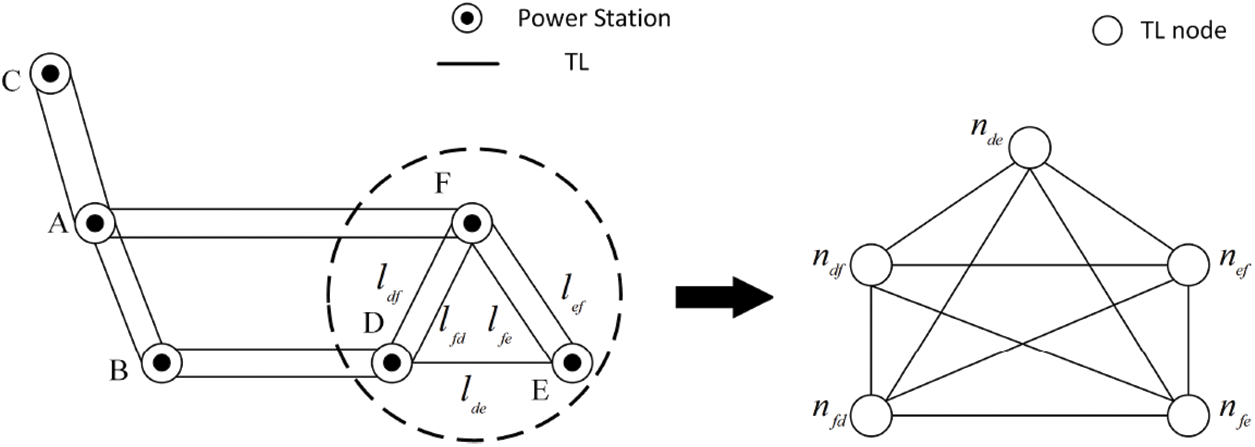
Figure 2: The topological structure of power grid branch is converted into the graph structure
Our proposed model can be divided into two modules, the encoding module STP-Block and the decoding module Multi-fitting-Block. Firstly, to deal with the mixing of transient data during the data collection process, the STP module uses average pooling for each feature of each grid node in a time window with a span of k to obtain the graph data of each time slice. Then, the module uses the node attention mechanism in GAT to calculate the attention coefficients of the node itself and its adjacent points according to the connection information of the power grid to mine the hidden structural information and integrate it into the features of the node to increase the dimension. Finally, put the dimension-raising information into Multi-fitting-Block. This module uses a hard-parameter-sharing strategy to build a multi-layer fully connected layer to predict the final parameters. Subsequent experiments show that the method is also accurate and robust in bad data.
Firstly, we should to explain the design considerations and theoretical basis of the STP module, and the first is the time-pool operation design consideration. In fact, traditional PI numerical method often considers the input SCADA cross-section data too ideally. Therefore, we must analyze the possible disturbances and abnormal situations in the SCADA measurement process to design the model structure. According to the reference [23], measurement disturbances and bad data usually have the following types:
• Transient data and steady-state data are mixed. As mentioned earlier, during the acquisition process, the terminal cannot judge whether the system is in a steady-state process, resulting in the measured value being either a steady-state value or a transient value.
• Power failure measured data loss. During the operation of the distribution network, there will be power failure of the transmission branch due to various reasons, such as lightning trips, maintenance, repair of the power-off line, and so on, which means terminal data cannot be collected at this time.
• Noise pollution. Acquisition devices are usually electronic sensing devices. Inevitably, the equipment will produce electromagnetic noise due to the environment.
According to reference [23], transient data mixing is the main reason for bad data. Therefore, our method mainly considers this factor to adjust the model composition. Generally, for rapidly changing data such as transient data, researchers use data smoothing to reduce the impact on model performance. Data smoothing can be divided into linear smoothing and nonlinear smoothing. Nonlinear smoothing requires finding a nonlinear function to estimate the branch data. Using nonlinear function to calculate each transient data point will undoubtedly bring substantial computational consumption. Therefore, we use mean linear smoothing to mitigate the impact of transient data. Subsequent experiments also found that the accuracy of the model proposed in this paper will not be greatly affected when the transient simulation data is mixed. In case of zero value of data loss, the influence can also be reduced through mean smoothing. As for noise interference, the neural network model can converge adaptively in adjusting regular parameters. This subsection first introduces the mathematical principle of GAT, which is the core of STP module, and analyzes why GAT should be selected. Secondly, we put forward the reasons for the emergence of transient data and the average pooling we use. Thirdly, we introduce the design and principle of multi-task decoding module.
Then, we need to describe the design considerations and theoretical basis for the operation of GAT to extract topologically constrained information in space. Our use of GAT to extract topology constraints has two advantages: (1) Considering information that is invariant under line data interference TLs’ connection constraints. (2) While extracting constraint information, the branch information is well integrated to lay the foundation for multi-branch identification.
GAT is a graph neural network proposed by Velivckovic [24]. Its core module uses Mask attention mechanism [25] to calculate node characteristics after fusion of spatial information. Suppose there is a graph
where W is learnable weight matrix,
In Eq. (7) LeakyReLU and
Through our Graph modeling method and GAT, each vertex of the graph structure will fuse the adjacent contact constraint information differently. In the TLs, the difference of the line each is usually very huge. Even if two wires with similar specifications are connected at the beginning and end of the same power station, their sag and environment must be different. This means that the model needs to consider the structural information on both sides of the same node asymmetrically. However, another popular graph neural network method GCN [26] is hard to consider node differences. Its hidden layer calculation formula is as follows:
where H is the lth middle layer information,
In summary, the workflow of our coding module STP module is shown in the Fig. 3. We construct a 3D tensor by splicing the graph data of each time acquisition section after graph modeling processing. The tensor length is the feature dimension, the width is the number of nodes, and the height is the time dimension. Each 2D section is a grid diagram data. We perform mean operation in the historical time window of k for each feature and input the GAT network to mine branch topology constraint information. The specific calculation process is as follows:

Figure 3: STP block introduce
Given a grid data at a certain time
where Concat is stitching operation, in that way matrix
Then we use GAT layer operation to fuse spatial information.
where D is degree matrix, information about temporal context and spatial topology has been incorporated by
Secondly, we elaborate on the design considerations and theoretical basis of the Multi-Fitting module. In fact, multi-branch PI is a multi-task objective. There are generally two solutions for multi-task goals. One is to use multiple isolated models to deal with multiple tasks redundantly, and the other is to use parameter-sharing thinking to combine multiple models so that the models can be widely used in various tasks. Branches’ data are strongly correlated with each other, and changes in electrical variables of a transmission branch often affect the measurement data of the entire distribution network. Multi-task learning [27] just utilizes the association and conflict between multiple tasks to realize multi-parameter identification.
As shown in the Fig. 4, the main network of multi task fitting block proposed in this paper is multi-layer FCN. Firstly, we use the hard parameter sharing strategy to flatten the tensor x processed above and input it into the shared layer for learning. Then, model separate the layers and tags of different tasks to complete the loss calculation. In the calculation, we consider that the multi task learning should not dominated or biased by a branch regression task. Therefore, this paper proposed a balanced regular loss function to balance the importance of the task. Finally, model fit the target to complete multi-parameters identification by continuous iteration. Specifically, the module will get the information of temporal and spatial constraint fusion after encoding STP block. Then, model perform MSE loss function calculation on the separated full connection layer and label:
where

Figure 4: Multi-fit block introduce
In fact, we only need a loss function with adaptive weighted multi branch loss which set to multiply the corresponding balance weight to pull the losses of all tasks to the same level during loss calculation. We design the loss balance function as follows:
Among that,

Figure 5: Loss comparison of different branches after self-balancing
As can be seen from the Fig. 5, the losses of different branches are multiplied by a set of weight parameters
According to the above introduction of the algorithm for transmission lines PI proposed in this paper, the overall process of the identification method proposed in this paper can be divided into three parts: 1) Data import and simulation condition setting; 2) STP-GTN model training; 3) Use trained model to identificate parameters and evaluate performance. The specific calculation steps are as follows, and the flowchart is shown in Fig. 6.
(1) The first part is data importing and simulation condition setting. We first initialize the parameters and simulation conditions used for training and testing. After importing the data measured by the SCADA system, we divide the data set according to the set test set ratio and add simulation conditions. Then, this paper uses the PyTorch-geometric [29] related interface to convert the grid data into graph data according to the graph modeling method mentioned above.
(2) Followed by the model training part. According to the setting of parameter k, we pool the graph and input it into STP-GTN for training, and set the evaluation threshold. Generally, we will stop after 200 rounds of training. To know iteration process has converged in advance, we add an early stop mechanism. If the evaluation indicators have not changed for a long time, we will stop training and temporarily save the model parameters.
(3) The last part is the testing and evaluation part. Like training, we input test graph data processed by pooling operation into the trained model for PI and calculation of evaluation indicators.

Figure 6: Flow chart of STP-GTN algorithm
3 Experimental Details and Result Discussion
3.1 Introduction of Branches Identification Data Set
The data set in this work are collected by the real SCADA system, which is provided by the China Electric Power Research Institute. The TLs network used is composed of 17 TL station nodes. The recorded data is arranged in chronological order by RTU. Each section data contains 7 features, and the features of all sections are processed by graph modeling method above. The data set consists of 8640 groups of data, and the recorder records the data every 1 s. Among them, 6700 groups of data are selected as the training set, and 1900 groups of data are selected as the test and verification.
The Table 1 and Fig. 7 show the general situation of data sources, which represents that the transmission nodes are far away, and the differences between branches are large. The characteristics of transmission lines are also quite different. In fact, this is the general situation in the existing power distribution network. Therefore, even if the machine learning and depth PI methods mentioned above do not consider how to splice the data of multiple branches, and force one model to complete the identification of multiple branches, the parameter distortion between tasks will also happen because of branches’ discrepancy.


Figure 7: Examples that illustrate the characteristic heterogeneity of different branches
3.2 Experimental Details and Benchmark Model
At the beginning of our research, we investigated the possible interference of PI data as mentioned above. Our design is based on the investigation of bad data. Considering the preciseness of the application method, the experimental design in this paper needs two parts: a) Considering the interference during training, and comparing the methods based on the same interference noise during testing. b) The simulation conditions of model training and test are different without considering the occurrence of interference during training. After such adjustment, if models in this paper still show strong robustness under these parts, we can talk about the specific application. The next section is arranged as follows: firstly, we visually describe the simulation interference conditions, then describe the process and benchmark of the experiment, and finally complete the details of the experiment.
We set three kinds of interference noise according to the investigation mentioned above. The first type is Gaussian noise in the acquisition process (we design Gaussian noise concerning Brown’s work [30]) as shown in Fig. 8a below. The second noise is power-off data loss (which refers to Kunjin Chen’s working noise [21]) as shown in Fig. 8b above. The third noise is a kind of transient data mixing shown in Fig. 8c.

Figure 8: Simulation of real environment
In order to deal with these three kinds of interference, before the final model is proposed in this paper, machine learning method and deep learning model are used successively in the whole experimental process. This is a gradual process: As far as the label-making theory in this paper is concerned, the parameter identification task essentially transformed by us into a regression task. Therefore, we first use six machine learning methods, such as linear regression, polynomial regression, ridge regression, SVR, XGBoost [31], LightGBM [32]. The above machine learning methods are used in the sklearn machine learning algorithm package. We use the cross validation method to obtain the hyperparameters of the model: the highest term of the calculation formula is considered to be 2 in the polynomial regression. SVR uses multi-core function after parameter adjustment, plus penalty factor c = 10, gama = 0.1. XGBoost is the fastest and best open-source boosting tree tool at present and also the benchmark with the best comprehensive performance in Kaggle regression competitions. The maximum iteration depth of XGBoost is 300, the learning rate is 0.01, the number of boost rounds is 300, and the degree of verbosity is false. LightGBM is the best gradient lifting algorithm among the time complexity optimization algorithms for XGBoost. We set the learning rate of LightGBM algorithm to 0.01 and the maximum iteration number to 200. Default parameters are best used in comparisons.
In addition, we also refer to some work on the intersection of DL and branch PI [33], and select three deep learning methods as benchmarks: full connection layer neural network (FCN) [20], convolution neural network (CNN) [34] and long-term and short-term memory neural network (LSTM) [35]. FCN makes full connection layer regression prediction of x by flattening the input matrix
Finally, other details about our experiment are described as follows: in this work, Adam [36] is selected as the neural network optimization algorithm. Unlike the traditional random gradient descent, Adam does not maintain a single learning rate in updating weights but uses the first-order moment estimation and second-order moment estimation of the gradient to design independent adaptive learning rates for different parameters. The Adam algorithm requires a small amount of memory. After offset correction, the learning rate of each iteration has a specific range, which makes the parameters relatively stable. For the measurement indicators, we use relative error to measure the advantages and disadvantages of the comparison model according to the particularity of the transmission network task. The reason is that we found that the order of magnitude of inductance G is
Among that,
3.3 Analysis and Discussion of Experimental Results
3.3.1 a) Pre Define Interference Limit during Test
The innovation and application of methods must consider the existing natural environment and can not just pursue the stacking of new methods and be divorced from reality. The method in this paper is proposed considering the insufficient data of general measurement process. In order to be rigorous, our experiment is divided into two steps: 1) pre-define the same training and testing conditions based on the bad data of survey measurement and compare the accuracy of the model; 2) do not pre-set the test simulation conditions, and the training and testing are based on different conditions to test the robustness of the model.
Here we need to mention our experimental process and ideas to inspire the follow-up work. Firstly, our initial idea is to develop a unified model to deal with multi-branch identification by using multi-task parameter sharing and modeling grid data into graph data. Secondly, considering the complexity of measurement noise, we want to improve the model fitting ability by stacking depth FCN. It is found that the method performance will decrease by
Table 2 shows that abbreviation LR (Linear Regression), PR (Polynomial Regression), RR (Ridge Regression). It can be seen from table above that the performance of traditional regression method is very good when there is no noise and only a small amount of Gaussian noise is added. The reason is also very simple: when the grid data is non-pollution, the traditional regression model will achieve high prediction accuracy. However, in the case of missing data and outliers, the traditional methods that rely on data purity fail, because the conditions of polynomial regression and ridge regression are very harsh, and the missing characteristics have a great impact on the results. Benefiting from XGBoost’s good fitting ability for residual terms, the overall performance is better than most of the machine learning algorithms we use when the noise is simple or no noise. However, in the case of complex noise, XGBoost and LightGBM have unstable identification parameters. This kind of gradient-boosting tree will have a sharp decline in performance when high-dimensional sparsity occurs, meaning features are missing. The disadvantages and advantages of each method can be clearly seen under a single noise. The parameter accuracy of LSTM and FCN, which depend on time sequence continuity, is reduced by 3 times in case of branch data loss or transient outlier data. CNN and our method converge well under a single condition.

Because noise usually does not appear singly, we add mixed complex noise. Under the condition of complex noise, our method performs best at the index level. The reason is that our method can take into account an invariant information structure constraint in the case of complex noise. Even in the case of data loss and transient outliers, our model can still mine the hidden structural attention in the branch. When the parameter interference of a single transmission line is serious, our method can mine the information of other branches to fill the interference loss through GAT coding so that the complex noise will not greatly impact the results. When the noise interference is large, the relative error of the method can be guaranteed to be less than
We post the convergence curve at the training stage as a visual demonstration in Fig. 9, where the left column represents the simple noise simulation environment, and the right column represents the complex noise. For comparison, we separately show the curve at the end of convergence at the bottom of two chart columns. Our method converged to an acceptable range at the end of the training process. However, other DL methods fluctuate violently, resulting in higher final calculated index than our model. So we think that these DL methods have weak anti-interference ability.

Figure 9: The relative error convergence curve of the deep learning algorithms, where column A represents the simple noise simulation environment, and column B represents the complex noise. Curve details means the convergence stage of training results, that is, the comparison after 100 generations
In fact, when we design the experiment, we consider bad data conditions in advance so that one of the advantages of our method can be shown in the compensation experiment. In the experiments without limited test interference conditions, our approach takes advantage of good robustness by considering invariance of spatial constraints.
3.3.2 b) Without Limited Test Interference Conditions
The model in this paper involves an operation of mean smoothing, which is an intermediate module designed based on the survey of bad data. In order to study rigorously, we must remove the conditional restrictions on bad parameters before training. Assuming that the actual test situation is not known during the training, the known condition training is used to optimize the weight of the super parameters and methods. Save the unknown test conditions of the model verification of the above links. Among them, the characters represent the meanings a (50 dB), A (100 dB), b (
Several conclusions can be drawn from the above Table 3. (1) Such training and predictive simulation settings are devastating for machine learning and traditional regression method. (2) Only the deep learning method has immunity under different train and test conditions. In the comparison of DL methods, the error of our method is about 2 times less than that of other methods. In fact, our method has strong robustness because we use graph modeling method and graph neural network to extract the only invariant spatial constraint information in complex interference.

For the problems of transient mixing and data contamination in data acquisition, the traditional numerical parameter identification method that relies too much on steady-state input and data purity may have the problem of identification distortion. This paper proposes a multi-branch parameter identification model considering topological constraints and transient data. Assuming that the grid data is essentially non-Euclidean data, the model uses graph modeling methods and graph neural networks to extract topology constraint information, which provides additional help for model robustness. Considering transient data in the collection process, this paper proposes a mean smoothing operation to reduce the influence of transient mixing on the identification results. Finally, this paper uses the parameter-sharing strategy and the self-balancing loss function to identify multiple branches with one model.
In experiments based on simulated data of natural SCADA systems, since this paper considers the topology constraint information that is invariant under the changing noise, the model can also have less relative error under the condition of complex noise. Specifically, we compared the model with fully connected neural network model (FCN) that without adding graph neural network layer, convolutional neural network (CNN), and long short memory network (LSTM) which depend on temporal integrity under different noise disturbances in training and testing. Still, our model shows better immunity.
However, our method needs to rely on the determined topological connection matrix. That means our model needs to reset the conditions and train when the grid adds new nodes, so we can only use the fixed branch structure. In the future, it is hoped that the dynamic graph neural network method can be used based on the graph modeling method in this paper to complete the parameter identification in the dynamic large-scale power grid.
Acknowledgement: The authors wish to express their appreciation to the reviewers for their helpful suggestions which greatly improved the presentation of this paper.
Funding Statement: This work is supported by the National Natural Science Foundation of PR China (42075130) and the Postgraduate Research and Innovation Project of Jiangsu Province (1534052101133).
Conflicts of Interest: The authors declare that they have no conflicts of interest to report regarding the present study.
References
1. Li, H., Xue, Y. S., Zhang, G. M. (2011). Influence of uncertainty of background parameters on parameter recognition. Power System Automation, 35(17), 10–13. [Google Scholar]
2. Ken, Y. E. (2004). Power system state estimation. Water Resources and Electric Power Press, 69(2), 3–4. [Google Scholar]
3. Debs, A. S. (1974). Estimation of steady-state power system model parameters. IEEE Transactions on Power Apparatus and Systems, 12(5), 1260–1268. https://doi.org/10.1109/TPAS.1974.293849 [Google Scholar] [CrossRef]
4. Slutsker, I. W., Mokhtari, S., Clements, K. A. (1996). Real time recursive parameter estimation in energy management systems. IEEE Transactions on Power Systems, 11(3), 1393–1399. https://doi.org/10.1109/59.535680 [Google Scholar] [CrossRef]
5. Bian, X. M., Qiu, J. J., Feng, X. X., (2008). Heuristic estimation of static line parameters in power system. Chinese Journal of Electrical Engineering, 28, 41–46. https://doi.org/10.13334/j.0258-8013.pcsee.2008.01.008 [Google Scholar] [CrossRef]
6. Wang, Z., Xia, M., Lu, M., Pan, L., Liu, J. (2022). Parameter identification in power transmission systems based on graph convolution network. IEEE Transactions on Power Delivery, 37(4), 3155–3163. https://doi.org/10.1109/TPWRD.2021.3124528 [Google Scholar] [CrossRef]
7. He, H., Chai, J. H. (2005). An improved parameter estimation method based on measurement residuals. Automation of Electric Power Systems, 31(4), 33–36. [Google Scholar]
8. Castillo, M. R., London, J. B., Bretas, N. G., Lefebvre, S., Lambert, B. (2010). Offline detection, identification, and correction of branch parameter errors based on several measurement snapshots. IEEE Transactions on Power Systems, 26(2), 870–877. https://doi.org/10.1109/TPWRS.2010.2061876 [Google Scholar] [CrossRef]
9. Ahmed, M. M., Soo, W. L. (2008). Supervisory control and data acquisition system (SCADA) based customized remote terminal unit (RTU) for distribution automation system. 2008 IEEE 2nd International Power and Energy Conference, pp. 1655–1660. Malaysia, IEEE. [Google Scholar]
10. Teixeira, A., Dán, G., Sandberg, H., Johansson, K. H. (2011). A cyber security study of a SCADA energy management system: Stealthy deception attacks on the state estimator. IFAC Proceedings Volumes, 44(1), 11271–11277. https://doi.org/10.3182/20110828-6-IT-1002.02210 [Google Scholar] [CrossRef]
11. Singh, D., Pandey, J. P., Chauhan, D. S. (2005). Topology identification, bad data processing, and state estimation using fuzzy pattern matching. IEEE Transactions on Power Systems, 20(3), 1570–1579. https://doi.org/10.1109/TPWRS.2005.852086 [Google Scholar] [CrossRef]
12. Angel, B., Duraisamy, M. (2022). Dynamic state estimation of electric power systems using kalman filtering techniques. Proceedings of Journal of Physics: Conference Series, 2335(1), 012053. https://doi.org/10.1088/1742-6596/2335/1/012053 [Google Scholar] [CrossRef]
13. Zhao, J., Fliscounakis, S., Panciatici, P., Mili, L. (2018). Robust parameter estimation of the French power system using field data. IEEE Transactions on Smart Grid, 10(5), 5334–5344. https://doi.org/10.1109/TSG.5165411 [Google Scholar] [CrossRef]
14. Liu, W. H., Wu, F. F., Lun, S. M. (1992). Estimation of parameter errors from measurement residuals in state estimation (power systems). IEEE Transactions on Power Systems, 7(1), 81–89. https://doi.org/10.1109/59.141690 [Google Scholar] [CrossRef]
15. Dobakhshari, A. S., Abdolmaleki, M., Terzija, V., Azizi, S. (2020). Online non-iterative estimation of transmission line and transformer parameters by SCADA data. IEEE Transactions on Power Systems, 36(3), 2632–2641. https://doi.org/10.1109/TPWRS.2020.3037997 [Google Scholar] [CrossRef]
16. Kong, H., Lu, M., Que, L., Xu, F., Zhao, J. et al. (2022). A new four step method to identify the parameters of transmission line based on SCADA data. IET Generation, Transmission Distribution, 16(9), 1822–1835. https://doi.org/10.1049/gtd2.12420 [Google Scholar] [CrossRef]
17. Pouyanfar, S., Sadiq, S., Yan, Y., Tian, H., Tao, Y. et al. (2018). A survey on deep learning: Algorithms, techniques, and applications. ACM Computing Surveys, 51(5), 1–36. [Google Scholar]
18. Lu, C., Xia, M., Lin, H. (2022). Multi-scale strip pooling feature aggregation network for cloud and cloud shadow segmentation. Neural Computing and Applications, 34(8), 6149–6162. https://doi.org/10.1007/s00521-021-06802-0 [Google Scholar] [CrossRef]
19. Que, L., Yang, L., Qian, H., Shen, J., Zhang, L. et al. (2020). A robust line parameter identification method based on LSTM and modified SCADA data. Proceedings of 2020 IEEE 4th Conference on Energy Internet and Energy System Integration (EI2), pp. 2981–2986. Wuhan, China, IEEE. [Google Scholar]
20. Lu, M., Jin, X., Wang, X., Xu, Y., Wang, Y. et al. (2020). A robust identification method for transmission line parameters based on BP neural network and modified SCADA data. Proceedings of 2020 IEEE International Conference on Energy Internet (ICEI), pp. 92–97. Wuhan, China. [Google Scholar]
21. Chen, K., Hu, J., Zhang, Y., Yu, Z., He, J. (2019). Fault location in power distribution systems via deep graph convolutional networks. IEEE Journal on Selected Areas in Communications, 38(1), 119–131. https://doi.org/10.1109/JSAC.49 [Google Scholar] [CrossRef]
22. Wang, Y., Xu, W., Shen, J. (2015). Online tracking of transmission-line parameters using SCADA data. IEEE Transactions on Power Delivery, 31(2), 674–682. https://doi.org/10.1109/TPWRD.2015.2474699 [Google Scholar] [CrossRef]
23. Hao, Y. S. (2012). Bad data mechanism and processing in telemetry data. China Southern Power Grid Technology, 6(5), 6. [Google Scholar]
24. Velickovic, P., Cucurull, G., Casanova, A., Romero, A., Lio, P. et al. (2017). Graph attention networks. Statistics, 1050, 20. https://doi.org/10.48550/arXiv.1710.10903 [Google Scholar] [CrossRef]
25. Qu, Y., Xia, M., Zhang, Y. (2021). Strip pooling channel spatial attention network for the segmentation of cloud and cloud shadow. Computers Geosciences, 157, 104940. https://doi.org/10.1016/j.cageo.2021.104940 [Google Scholar] [CrossRef]
26. Kipf, T. N., Welling, M. (2016). Semi-supervised classification with graph convolutional networks. Computer Science. https://doi.org/10.48550/arXiv.1609.02907 [Google Scholar] [CrossRef]
27. Caruana, R. (1997). Multitask learning. Machine Learning, 28(1), 41–75. https://doi.org/10.1023/A:1007379606734 [Google Scholar] [CrossRef]
28. Ruder, S. (2017). An overview of multi-task learning in deep neural networks. Computer Science. https://doi.org/10.48550/arXiv.1706.05098 [Google Scholar] [CrossRef]
29. Fey, M., Lenssen, J. E. (2019). Fast graph representation learning with PyTorch Geometric. Computer Science. https://doi.org/10.48550/arXiv.1903.02428 [Google Scholar] [CrossRef]
30. Brown, M., Biswal, M., Brahma, S., Ranade, S. J., Cao, H. (2016). Characterizing and quantifying noise in PMU data. 2016 IEEE Power and Energy Society General Meeting (PESGM), pp. 1–5. Boston, IEEE. [Google Scholar]
31. Chen, T., Guestrin, C. (2016). XGBoost: A scalable tree boosting system. Proceedings of the 22nd acm Sigkdd International Conference on Knowledge Discovery and Data Mining, pp. 785–794. San Francisco. https://doi.org/10.1145/2939672.2939785 [Google Scholar] [CrossRef]
32. Ke, G., Meng, Q., Finley, T., Wang, T., Chen, W. et al. (2017). Lightgbm: A highly efficient gradient boosting decision tree. Proceedings of the 31st Conference on Neural Information Processing Systems (NIPS 2017), pp. 3149–3157. Long Beach, CA, USA. [Google Scholar]
33. Ning, L., Sun, H. B., Wu, W. Z., Zhang, B. M. (2009). State estimation based branch parameter estimation method for power grid. Proceedings of the CSEE, 29(1), 7–13. [Google Scholar]
34. Kattenborn, T., Leitloff, J., Schiefer, F., Hinz, S. (2021). Review on convolutional neural networks (CNN) in vegetation remote sensing. ISPRS Journal of Photogrammetry and Remote Sensing, 173, 24–49. https://doi.org/10.1016/j.isprsjprs.2020.12.010 [Google Scholar] [CrossRef]
35. Graves, A. (2012). Long short-term memory. Supervised Sequence Labelling with Recurrent Neural Networks, 37–45. https://doi.org/10.1007/978-3-642-24797-24 [Google Scholar] [CrossRef]
36. Kingma, D. P., Ba, J. (2014). Adam: A method for stochastic optimization. Computer Science. https://doi.org/10.48550/arXiv.1412.6980 [Google Scholar] [CrossRef]
Cite This Article
 Copyright © 2023 The Author(s). Published by Tech Science Press.
This work is licensed under a Creative Commons Attribution 4.0 International License , which permits unrestricted use, distribution, and reproduction in any medium, provided the original work is properly cited.
 Downloads
 Citation Tools