1 Introduction
Physical and technical workflows are recognized by fractional calculus (FC) and are succinctly explained by fractional differential equations (FDEs) [1–4]. Admittedly, classical simulation results of integer-order derivatives, which include empirical systems, do not underlie well in numerous situations [5–9]. FC has contributed substantially to quantum physics, nuclear magnetic resonance, image recognition, circuit theory, transport phenomena, chaos, and epidemiology. Diverse aspects of FC have been researched by Kilbas et al. [10–14].
Fractional differential equations (FDEs) are viewed as the most vital and effective mechanism for describing and modeling complex anomalies in general, such as seismic nonlinear vibration. Because of the revelation of fractal frameworks in finance, many researchers have examined fractional configurations in recent years. FDEs are also employed to simulate computational anatomy, biochemical mechanisms, and a variety of other natural or physical structures [15–19]. Nonlinear problems are interesting to architects, astronomers, and cosmologists since most physical processes in nature are nonlinear. On the other hand, nonlinear equations are complicated to fix and can yield fascinating results [20–26]. In the analysis of high-order nonlinear equations, the actual solutions of transition models contribute significantly.
Even so, humanity is constantly seeking improvements in correctness or accuracy, computation complexity, trustworthiness and appropriateness. Recently, Tarig Elzaki envisioned the Elazki transform (E-transform) by merging well-noted transforms, the Laplace and Sumudu transformations. It can indubitably strengthen the quantitative expression of differential equations in the same way that Laplace and Sumudu transformations have. The E-transform is developed from the traditional Fourier integral, with emphasis on its computational adaptability and promising effects. The E-transform is aimed at resolving ordinary and PDEs in the time realm. The Fourier, Laplace, and Sumudu transforms, in particular, are impacting, pragmatic computational methodologies for addressing FDEs. It is worth noting that the E-transformation was formerly recommended over an ancient, more intricate methodology, including the Sumudu technique. Nonetheless, we need to show that the Elzaki transformation can resolve issues that Laplace cannot [27]. In this article, the E-transform is used to reconfigure the iterative algorithm, and the novel paradigm is known as the “Elzaki Adomian Decomposition Method (EADM).”
Mathematicians have progressively focused their consideration on approximate and analytical solutions to PDEs for developing advanced mathematical strategies address PDEs. Some well acquainted strategies concerning the solution of PDEs are the homotopy analysis method (HAM), new iteration method (NIM), Laplace transform algorithm (LTA), the Haar wavelet technique (HWT) and many more.
In 1982, the Navier-Stokes equation (NSe) was first devised by Navier [28]. The equation is a confluence of the momentum equation, the continuity equation, and the energy equation, and it can be considered Newton’s second law of motion for fluid substances. The NS-model is significant because it explains a variety of interesting physical phenomena that occur in various areas of applied sciences, such as ocean circulation, atmosphere, air circulation across awing, and hydrological cycle in tubes, see [29,30].
Several researchers have attempted to solve the NSe problem using various approaches. To efficiently strengthen the algorithmic structure, Eltayeb et al. [31] proposed unifying the multi-Laplace transform decomposition method for NSe. Shah et al. [32] presented the analytical solution of NSe utilizing the natural transform decomposition method. Singh et al. [33] have expounded numerical simulation by considering fractional reduced differential transformation method for discovering an analytical solution of the time-fractional model of NSe. Khan et al. [34] introduced the Elzaki transform decomposition approach for finding the analytical solution of NSe.
Inspired by the work of [31,34], we aim to investigate the multi-dimensional time fractional model of NSe with the aid of triple Elzaki Adomian decomposition method (TEADM) and quadruple Elzaki Adomian decomposition method (QEADM). Elzaki transformation [35,36] and Adomian decomposition method (ADM) [37,38] are incorporated in the suggested framework. For the formulations of quantitative and qualitative analysis, the Elzaki transformation [39–41] and ADM [37,38] have been utilized independently and supply the exact solutions in terms of convergent series. The exact and approximated solution of nonlinear NSe are addressed using advanced technique. With the assistance of graphs, the findings are illustrated and validated. The new approach is demonstrated to solve fractional-order equations in a quite clear and concise way. Other modulation problems in different fields of mathematical and physical sciences can be addressed using the current approach.
The structure of the article is as follows: Section 2 represents the basic definitions related to fractional calculus and the proposed Elzaki transform. Section 3 illustrates the road map for the analytical approximations of triple and quadruple Elzaki Adomian decomposition methods. Numerical experiments and their graphical illustrations concerning the TEADM and QEADM are conducted in Section 4. Theoretical findings are elaborated via comparison analysis with the previous findings demonstrated in Section 5. In a nutshell, we summarized the concluding remarks with open problems.
2 Prelude
In this unit, we have addressed several of the key aspects of FC and triple Elzaki transform. For more details, see [10,12].
The Elzaki transform [35] is a novel integral operator described for functions of exponential order. We shall look at mappings in the set G that are specified by
G={ℏ(ξ):∃ℳ,κ1,κ2>0;|ℏ(ξ)|<ℳe|ξ|κ;ξ∈(−1)ȷ×[0,+∞)}.
Definition 2.1. ([35]) Elzaki transform for function ℏ(ξ) is defined as
E[ℏ(ξ)]=ℋ(p)=p∫0+∞ℏ(ξ)e−ξpdξ,ξ>0,κ1<p<κ2.(1)
This transform has a stronger resemblance to the Laplace transform such as ℒ(s)=ηE(1η). The Elzaki transform is an efficient tool for providing the solution of integral equations, FDEs and PDEs.
Now we define the triple Elzaki transform as follows:
Definition 2.2. For ϖ1,ϖ2,ξ>0 and let ℏ be a mapping of three variables ϖ1,ϖ2 and ξ. Then the triple Elzaki transform of ℏ is stated as
Eϖ1Eϖ2Eξ[ℏ(ϖ1,ϖ2,ξ)]=ℋ(η,ζ,s)=ηζs∫0+∞∫0+∞∫0+∞ℏ(ϖ1,ϖ2,ξ)e−ϖ1η−ϖ2ζ−ξsdξdϖ2dϖ1,(2)
where η,ζ,s∈(κ1,κ2). Also, the triple Elzaki transforms of the first and second order partial derivatives are presented by
Eϖ1Eϖ2Eξ[ℏϖ1(ϖ1,ϖ2,ξ)]=1ηℋ(η,ζ,s)−ℋ(0,ζ,s),Eϖ1Eϖ2Eξ[ℏϖ2(ϖ1,ϖ2,ξ)]=1ζℋ(η,ζ,s)−ℋ(η,0,s),Eϖ1Eϖ2Eξ[ℏξ(ϖ1,ϖ2,ξ)]=1sℋ(η,ζ,s)−ℋ(η,ζ,0).(3)
Analogously, we have
Eϖ1Eϖ2Eξ[ℏϖ1ϖ1(ϖ1,ϖ2,ξ)]=1η2ℋ(η,ζ,s)−ℋ(0,ζ,s)−ηℏϖ1(0,ζ,s),Eϖ1Eϖ2Eξ[ℏϖ2ϖ2(ϖ1,ϖ2,ξ)]=1ζ2ℋ(η,ζ,s)−ℋ(η,0,s)−ζℏϖ1(η,0,s),Eϖ1Eϖ2Eξ[ℏξξ(ϖ1,ϖ2,ξ)]=1s2ℋ(η,ζ,s)−ℋ(η,ζ,0)−sℏϖ1(η,ζ,0).(4)
The inverse triple Elzaki transform Eη−1Eζ−1Es−1[ℋ(η,ζ,s)]=ℏ(ϖ1,ϖ2,ξ) is stated as follows:
ℏ(ϖ1,ϖ2,ξ)=Eη−1Eζ−1Es−1[ℋ(η,ζ,s)]=ηζs∫0+∞∫0+∞∫0+∞eηϖ1+ζϖ2+sξE(1η)E(1ζ)E(1s)dηdζds.(5)
Definition 2.3. ([13]) The Caputo fractional operator of a function ℏ of order ϕ>0 can be stated as follows:
c𝒟ϕℏ(ϖ1)={1Γ(ℓ−ϕ)∫0ϖ1(ϖ1−ξ)ℓ−ϕ−1ℏ(ξ)dξ,ℓ−1<ϕ<ℓ,dℓdϖ1ℓℏ(ϖ1)ℓ=ϕ.
Our next result is important for further investigation of this article.
Theorem 2.1. For ϕ1,ϕ2,ϕ3>0,ℓ−1<ϕ1≤ℓ,n−1<ϕ2≤n,q−1<ϕ3≤q and ℓ,n,q∈N, so that f1∈Ci(R+×R+×R+),i=max{ℓ,n,q},f1(i)∈L1[(0,a1)×(0,b1)×(0,c1)] for any a1,b1,c1>0,|f1(ϖ1,ϖ2,q)|≤ℳeϖ1ξ1+ϖ2ξ2+ϖ3ξ3,0<a1<ϖ1,0<b1<ϖ2,0<c1<ξ, then the triple Elzaki transforms of Caputo’s fractional derivatives 𝒟ξϕ1ℏ(ϖ1,ϖ2,ξ),𝒟ξϕ2ℏ(ϖ1,ϖ2,ξ) and 𝒟ξϕ3ℏ(ϖ1,ϖ2,ξ) are described by
Eϖ1Eϖ2Eξ[𝒟ξϕ1ℏ(ϖ1,ϖ2,ξ)]=s−ϕ1ℋ(η,ζ,s)−∑i=0ℓ−1s2−ϕ1+iEϖ2Eϖ1[𝒟ξiℏ(ϖ1,ϖ2,0)],ℓ−1<ϕ1<ℓ,Eϖ1Eϖ2Eξ[𝒟ϖ2ϕ2ℏ(ϖ1,ϖ2,ξ)]=ζ−ϕ2ℋ(η,ζ,s)−∑j=0n−1ζ2−ϕ2+jEϖ1Eξ[𝒟ϖ2jℏ(ϖ1,0,ξ)],n−1<ϕ2<n
and
Eϖ1Eϖ2Eξ[𝒟ϖ1ϕ3ℏ(ϖ1,ϖ2,ξ)]=η−ϕ3ℋ(η,ζ,s)−∑κ=0q−1η2−ϕ3+κEϖ2Eξ[𝒟ϖ1κℏ(0,ϖ2,ξ)],q−1<ϕ3<q.
3 Description of the Method for Triple Elzaki Transform Decomposition Method
The constructive approach of the TEADM for multi-dimensional time-fractional NSe is presented in this section. Assume the following framework of two-dimensional time-fractional NSe to demonstrate the underlying strategy of the TEADM:
∂ϕΦ∂ξϕ+Φ∂Φ∂ϖ1+Ψ∂Φ∂ϖ2=ρ0(∂2Φ∂ϖ12+∂2Φ∂ϖ22)+1ρ∂σ∂ϖ1,ϖ1,ϖ2,ξ>0,∂ϕΨ∂ξϕ+Φ∂Ψ∂ϖ1+Ψ∂Ψ∂ϖ2=ρ0(∂2Ψ∂ϖ12+∂2Ψ∂ϖ22)−1ρ∂σ∂ϖ2,ϖ1,ϖ2,ξ>0,(6)
subject to
Φ(ϖ1,ϖ2,0)=f1(ϖ1,ϖ2),Ψ(ϖ1,ϖ2,0)=g1(ϖ1,ϖ2),
where ∂ϕ∂ξϕ is the Caputo fractional derivative and σ is the pressure. Also, if σ is known, then ℏ1=1ρ∂σ∂ϖ1 and ℏ2=1ρ∂σ∂ϖ2. To employ the TEADM, multiply (6) by ϖ1, which leads us
1sϕEϖ1Eϖ2Eξ[Φ(ϖ1,ϖ2,ξ)]−∑κ=0ℓ−1Φ(κ)(η,ζ,0)s2−ϕ+κ=−Eϖ1Eϖ2Eξ(Φ∂Φ∂ϖ1+Ψ∂Φ∂ϖ2)+Eϖ1Eϖ2Eξ(ρ0(∂2Φ∂ϖ12+∂2Φ∂ϖ22)+ℏ1),1sϕEϖ1Eϖ2Eξ[Ψ(ϖ1,ϖ2,ξ)]−∑κ=0ℓ−1Ψ(κ)(η,ζ,0)s2−ϕ+κ=−Eϖ1Eϖ2Eξ(Φ∂Ψ∂ϖ1+Ψ∂Ψ∂ϖ2)+Eϖ1Eϖ2Eξ(ρ0(∂2Ψ∂ϖ12+∂2Ψ∂ϖ22))−Eϖ1Eϖ2Eξ(ℏ2).(7)
By the virtue of Theorem 2.1, we obtain
Eϖ1Eϖ2Eξ[Φ(ϖ1,ϖ2,ξ)]=s2ℱ1(η,ζ)−sϕEϖ1Eϖ2Eξ(Φ∂Φ∂ϖ1+Ψ∂Φ∂ϖ2)+sϕEϖ1Eϖ2Eξ(ρ0(∂2Φ∂ϖ12+∂2Φ∂ϖ22))+sϕEϖ1Eϖ2Eξ(ℏ1),Eϖ1Eϖ2Eξ[Ψ(ϖ1,ϖ2,ξ)]=s2𝒢1(η,ζ)−sϕEϖ1Eϖ2Eξ(Φ∂Ψ∂ϖ1+Ψ∂Ψ∂ϖ2)+sϕEϖ1Eϖ2Eξ(ρ0(∂2Ψ∂ϖ12+∂2Ψ∂ϖ22))−sϕEϖ1Eϖ2Eξ(ℏ2).(8)
By implementing the triple inverse Elzaki transformation for (8), we obtain
Φ(ϖ1,ϖ2,ξ)=Eη−1Eζ−1Es−1[s2ℱ1(η,ζ)−sϕEϖ1Eϖ2Eξ(Φ∂Φ∂ϖ1+Ψ∂Φ∂ϖ2)+sϕEϖ1Eϖ2Eξ(ρ0(∂2Φ∂ϖ12+∂2Φ∂ϖ22))+sϕEϖ1Eϖ2Eξ(ℏ1)],Ψ(ϖ1,ϖ2,ξ)=Eη−1Eζ−1Es−1[s2𝒢1(η,ζ)−sϕEϖ1Eϖ2Eξ(Φ∂Ψ∂ϖ1+Ψ∂Ψ∂ϖ2)+sϕEϖ1Eϖ2Eξ(ρ0(∂2Ψ∂ϖ12+∂2Ψ∂ϖ22))−sϕEϖ1Eϖ2Eξ(ℏ2)].(9)
The infinite series solutions Φ(ϖ1,ϖ2,ξ) and Ψ(ϖ1,ϖ2,ξ) are presented as follows:
Φ(ϖ1,ϖ2,ξ)=∑ℓ=0+∞Φℓ(ϖ1,ϖ2,ξ),Ψ(ϖ1,ϖ2,ξ)=∑ℓ=0+∞Ψℓ(ϖ1,ϖ2,ξ).(10)
Meanwhile, the non-linear expressions 𝒩1=Φ∂Φ∂ϖ1,𝒩2=Ψ∂Φ∂ϖ2,𝒩3=Φ∂Ψ∂ϖ1 and 𝒩4=Ψ∂Ψ∂ϖ2 are denoted by
𝒩1(Φ,Ψ)=∑ℓ=0+∞𝒜ℓ,𝒩2(Φ,Ψ)=∑ℓ=0+∞ℬℓ,𝒩3(Φ,Ψ)=∑ℓ=0+∞𝒞ℓ,𝒩4(Φ,Ψ)=∑ℓ=0+∞𝒟ℓ(11)
and are presented by the Adomian polynomials as
𝒜ℓ=1ℓ![∂ℓ∂θℓ{𝒩1(∑κ=0+∞θκΦκ,∑κ=0+∞θκΨκ)}]θ=0,ℬℓ=1ℓ![∂ℓ∂θℓ{𝒩2(∑κ=0+∞θκΦκ,∑κ=0+∞θκΨκ)}]θ=0,𝒞ℓ=1ℓ![∂ℓ∂θℓ{𝒩3(∑κ=0+∞θκΦκ,∑κ=0+∞θκΨκ)}]θ=0,𝒟ℓ=1ℓ![∂ℓ∂θℓ{𝒩4(∑κ=0+∞θκΦκ,∑κ=0+∞θκΨκ)}]θ=0.(12)
By inserting (12) into (9), we attain
Eϖ1Eϖ2Eξ[∑ℓ=0+∞Φℓ(ϖ1,ϖ2,ξ)]=s2ℱ1(η,ζ)−sϕEϖ1Eϖ2Eξ(∑ℓ=0+∞(𝒜ℓ+ℬℓ))+sϕEϖ1Eϖ2Eξ(ρ0(∑ℓ=0+∞∂2Φℓ∂ϖ12+∑ℓ=0+∞∂2Φℓ∂ϖ22))+sϕEϖ1Eϖ2Eξ(ℏ1)(13)
and
Eϖ1Eϖ2Eξ[∑ℓ=0+∞Ψℓ(ϖ1,ϖ2,ξ)]=s2𝒢1(η,ζ)−sϕEϖ1Eϖ2Eξ(∑ℓ=0+∞(𝒞ℓ+𝒟ℓ))+sϕEϖ1Eϖ2Eξ(ρ0(∑ℓ=0+∞∂2Ψℓ∂ϖ12+∑ℓ=0+∞∂2Ψℓ∂ϖ22))−sϕEϖ1Eϖ2Eξ(ℏ2).(14)
By implementing the inverse Elzaki transformation to (13) and (14) we have
∑ℓ=0+∞Φℓ(ϖ1,ϖ2,ξ)=Eη−1Eζ−1Es−1[s2ℱ1(η,ζ)]−Eη−1Eζ−1Es−1[sϕEϖ1Eϖ2Eξ(∑ℓ=0+∞(𝒜ℓ+ℬℓ))]+Eη−1Eζ−1Es−1[sϕEϖ1Eϖ2Eξ(ρ0(∑ℓ=0+∞∂2Φℓ∂ϖ12+∑ℓ=0+∞∂2Φℓ∂ϖ22))+sϕEϖ1Eϖ2Eξ(ℏ1)](15)
and
∑ℓ=0+∞Ψℓ(ϖ1,ϖ2,ξ)=Eη−1Eζ−1Es−1[s2𝒢1(η,ζ)]−Eη−1Eζ−1Es−1[sϕEϖ1Eϖ2Eξ(∑ℓ=0+∞(𝒞ℓ+𝒟ℓ))]+Eη−1Eζ−1Es−1[sϕEϖ1Eϖ2Eξ(ρ0(∑ℓ=0+∞∂2Ψℓ∂ϖ12+∑ℓ=0+∞∂2Ψℓ∂ϖ22))−sϕEϖ1Eϖ2Eξ(ℏ2)].(16)
Taking into account the TEADM, we develop iterative connections as follows:
Φ0(ϖ1,ϖ2,ξ)=Eη−1Eζ−1Es−1[s2ℱ1(η,ζ)],Ψ0(ϖ1,ϖ2,ξ)=Eη−1Eζ−1Es−1[s2𝒢1(η,ζ)],(17)
and the rest of the components Φℓ+1,ℓ≥0 are presented by
Φℓ+1(ϖ1,ϖ2,ξ)=−Eη−1Eζ−1Es−1[sϕEϖ1Eϖ2Eξ(𝒜ℓ+ℬℓ)]+Eη−1Eζ−1Es−1[sϕEϖ1Eϖ2Eξ(ρ0(∂2Φℓ∂ϖ12+∂2Φℓ∂ϖ22))+sϕEϖ1Eϖ2Eξ(ℏ1)].(18)
and
Ψℓ+1(ϖ1,ϖ2,ξ)=−Eη−1Eζ−1Es−1[sϕEϖ1Eϖ2Eξ(𝒞ℓ+𝒟ℓ)]+Eη−1Eζ−1Es−1[sϕEϖ1Eϖ2Eξ(ρ0(∂2Ψℓ∂ϖ12+∂2Ψℓ∂ϖ22))−sϕEϖ1Eϖ2Eξ(ℏ2)].(19)
where Eϖ1Eϖ2Eξ is the triple E-transform in respecting ϖ1,ϖ2,ξ1 and Eη−1Eζ−1Es−1 is the triple inverse E-transform in respecting η,ζ,s. For (17)–(19), we assumed that the triple inverse E-transform exists.
4 Application of the Proposed Method
In this section, we evaluate the efficacy of our current techniques by introducing the decomposition method in combination with the triple and quadruple E-transform.
Problem 4.1. We assume the two dimensional time-fractional NSe:
{∂ϕΦ∂ξϕ+Φ∂Φ∂ϖ1+Ψ∂Φ∂ϖ2=ρ(∂2Φ∂ϖ12+∂2Φ∂ϖ22)+ℏ,ϖ1,ϖ2,ξ>0,∂ϕΨ∂ξϕ+Φ∂Ψ∂ϖ1+Ψ∂Ψ∂ϖ2=ρ(∂2Ψ∂ϖ12+∂2Ψ∂ϖ22)−ℏ,ϖ1,ϖ2,ξ>0,ℓ−1<ϕ<ℓ;(20)
subject to
{Φ(ϖ1,ϖ2,0)=−sin(ϖ1+ϖ2),Ψ(ϖ1,ϖ2,0)=sin(ϖ1+ϖ2).(21)
Proof. By applying the triple Elzaki transform on (20), we have
Eϖ1Eϖ2Eξ[∂ϕΦ∂ξϕ+Φ∂Φ∂ϖ1+Ψ∂Φ∂ϖ2]=Eϖ1Eϖ2Eξ[ρ(∂2Φ∂ϖ12+∂2Φ∂ϖ22)+ℏ],Eϖ1Eϖ2Eξ[∂ϕΨ∂ξϕ+Φ∂Ψ∂ϖ1+Ψ∂Ψ∂ϖ2]=Eϖ1Eϖ2Eξ[ρ(∂2Ψ∂ϖ12+∂2Ψ∂ϖ22)−ℏ].
On making the use of differentiation property of the Elzaki transform, we obtain
1sϕEϖ1Eϖ2Eξ[Φ(ϖ1,ϖ2,ξ)]−∑κ=0ℓ−1Φ(κ)(η,ζ,0)s2−ϕ+κ=−Eϖ1Eϖ2Eξ[Φ∂Φ∂ϖ1+Ψ∂Φ∂ϖ2]+Eϖ1Eϖ2Eξ[ρ(∂2Φ∂ϖ12+∂2Φ∂ϖ22)+ℏ],1sϕEϖ1Eϖ2Eξ[Ψ(ϖ1,ϖ2,ξ)]−∑κ=0ℓ−1Ψ(κ)(η,ζ,0)s2−ϕ+κ=−Eϖ1Eϖ2Eξ[Φ∂Ψ∂ϖ1+Ψ∂Ψ∂ϖ2]+Eϖ1Eϖ2Eξ[ρ(∂2Ψ∂ϖ12+∂2Ψ∂ϖ22)−ℏ].(22)
According to initial conditions and simple computations yields
Eϖ1Eϖ2Eξ[Φ(ϖ1,ϖ2,ξ)]=−s2Eϖ1Eϖ2[sin(ϖ1+ϖ2)]−sϕEϖ1Eϖ2Eξ[Φ∂Φ∂ϖ1+Ψ∂Φ∂ϖ2]+sϕEϖ1Eϖ2Eξ[ρ(∂2Φ∂ϖ12+∂2Φ∂ϖ22)+ℏ],Eϖ1Eϖ2Eξ[Ψ(ϖ1,ϖ2,ξ)]=s2Eϖ1Eϖ2[sin(ϖ1+ϖ2)]−sϕEϖ1Eϖ2Eξ[Φ∂Ψ∂ϖ1+Ψ∂Ψ∂ϖ2]+sϕEϖ1Eϖ2Eξ[ρ(∂2Ψ∂ϖ12+∂2Ψ∂ϖ22)−ℏ].
Eϖ1Eϖ2Eξ[Φ(ϖ1,ϖ2,ξ)]=−s2η2ζ2(η+ζ)(η2+1)(ζ2+1)−sϕEϖ1Eϖ2Eξ[Φ∂Φ∂ϖ1+Ψ∂Φ∂ϖ2]+sϕEϖ1Eϖ2Eξ[ρ(∂2Φ∂ϖ12+∂2Φ∂ϖ22)+ℏ],Eϖ1Eϖ2Eξ[Ψ(ϖ1,ϖ2,ξ)]=s2η2ζ2(η+ζ)(η2+1)(ζ2+1)−sϕEϖ1Eϖ2Eξ[Φ∂Ψ∂ϖ1+Ψ∂Ψ∂ϖ2]+sϕEϖ1Eϖ2Eξ[ρ(∂2Ψ∂ϖ12+∂2Ψ∂ϖ22)−ℏ].(23)
Employing the inverse triple Elzaki transform for (23)
Φ(ϖ1,ϖ2,ξ)=−sin(ϖ1+ϖ2)+Eη−1Eζ−1Es−1[sϕEϖ1Eϖ2Eξ(ℏ)]−Eη−1Eζ−1Es−1[sϕEϖ1Eϖ2Eξ[Φ∂Φ∂ϖ1+Ψ∂Φ∂ϖ2]]+Eη−1Eζ−1Es−1[sϕEϖ1Eϖ2Eξ[ρ(∂2Φ∂ϖ12+∂2Φ∂ϖ22)]],Ψ(ϖ1,ϖ2,ξ)=sin(ϖ1+ϖ2)−Eη−1Eζ−1Es−1[sϕEϖ1Eϖ2Eξ(ℏ)]−Eη−1Eζ−1Es−1[sϕEϖ1Eϖ2Eξ[Φ∂Ψ∂ϖ1+Ψ∂Ψ∂ϖ2]]+Eη−1Eζ−1Es−1[sϕEϖ1Eϖ2Eξ[ρ(∂2Ψ∂ϖ12+∂2Ψ∂ϖ22)]].(24)
It follows that
Φ(ϖ1,ϖ2,ξ)=−sin(ϖ1+ϖ2)+Eη−1Eζ−1Es−1[ℏη2ς2sϕ+2]−Eη−1Eζ−1Es−1[sϕEϖ1Eϖ2Eξ[Φ∂Φ∂ϖ1+Ψ∂Φ∂ϖ2]]+Eη−1Eζ−1Es−1[sϕEϖ1Eϖ2Eξ[ρ(∂2Φ∂ϖ12+∂2Φ∂ϖ22)]],Ψ(ϖ1,ϖ2,ξ)=sin(ϖ1+ϖ2)−Eη−1Eζ−1Es−1[ℏη2ς2sϕ+2]−Eη−1Eζ−1Es−1[sϕEϖ1Eϖ2Eξ[Φ∂Ψ∂ϖ1+Ψ∂Ψ∂ϖ2]]+Eη−1Eζ−1Es−1[sϕEϖ1Eϖ2Eξ[ρ(∂2Ψ∂ϖ12+∂2Ψ∂ϖ22)]].(25)
Consequently, we have
Φ(ϖ1,ϖ2,ξ)=−sin(ϖ1+ϖ2)+ℏξϕΓ(ϕ+1)−Eη−1Eζ−1Es−1[sϕEϖ1Eϖ2Eξ[Φ∂Φ∂ϖ1+Ψ∂Φ∂ϖ2]]+Eη−1Eζ−1Es−1[sϕEϖ1Eϖ2Eξ[ρ(∂2Φ∂ϖ12+∂2Φ∂ϖ22)]],Ψ(ϖ1,ϖ2,ξ)=sin(ϖ1+ϖ2)−ℏξϕΓ(ϕ+1)−Eη−1Eζ−1Es−1[sϕEϖ1Eϖ2Eξ[Φ∂Ψ∂ϖ1+Ψ∂Ψ∂ϖ2]]+Eη−1Eζ−1Es−1[sϕEϖ1Eϖ2Eξ[ρ(∂2Ψ∂ϖ12+∂2Ψ∂ϖ22)]].(26)
The infinite series solution for unknown function Φ(ϖ1,ϖ2,ξ) and Ψ(ϖ1,ϖ2,ξ) have the following form:
Φ(ϖ1,ϖ2,ξ)=∑ℓ=0+∞Φℓ(ϖ1,ϖ2,ξ),Ψ(ϖ1,ϖ2,ξ)=∑ℓ=0+∞Ψℓ(ϖ1,ϖ2,ξ).(27)
The Adomian approach is required to determine the zeroth elements Φ0 and Ψ0. Therefore, it includes initial condition, all of which are considered to be identified. Consequently, we devised
Φ0=−sin(ϖ1+ϖ2)+ℏξϕΓ(ϕ+1),Ψ0=sin(ϖ1+ϖ2)−ℏξϕΓ(ϕ+1).
Remember that Φ∂Φ(ϖ1,ξ)∂ϖ1=∑ℓ=0+∞𝒜ℓ, Ψ∂Φ(ϖ1,ξ)∂ϖ2=∑ℓ=0+∞ℬℓ, Φ∂Ψ(ϖ1,ξ)∂ϖ1=∑ℓ=0+∞𝒞ℓ and Ψ∂Ψ(ϖ1,ξ)∂ϖ2=∑ℓ=0+∞𝒟ℓ are the Adomian terms and nonlinear terms were characterized. Now, (26) can be expressed in an iterative way with the aid of (27), as follows:
∑ℓ=0+∞Φℓ(ϖ1,ϖ2,ξ)=−Eη−1Eζ−1Es−1[sϕEϖ1Eϖ2Eξ[∑ℓ=0+∞𝒜ℓ+∑ℓ=0+∞ℬℓ]]+Eη−1Eζ−1Es−1[sϕEϖ1Eϖ2Eξ[ρ(∂2Φℓ∂ϖ12+∂2Φℓ∂ϖ22)]],∑ℓ=0+∞Ψℓ(ϖ1,ϖ2,ξ)=−Eη−1Eζ−1Es−1[sϕEϖ1Eϖ2Eξ[∑ℓ=0+∞𝒞ℓ+∑ℓ=0+∞𝒟ℓ]]+Eη−1Eζ−1Es−1[sϕEϖ1Eϖ2Eξ[ρ(∂2Ψℓ∂ϖ12+∂2Ψℓ∂ϖ22)]].
Thanks to (11), the Adomian polynomials will express all forms of nonlinearity as
𝒜0=Φ0∂Φ0∂ϖ1,𝒜1=Φ0∂Φ1∂ϖ1+Φ1∂Φ0∂ϖ1,𝒜2=Φ0∂Φ2∂ϖ1+Φ1∂Φ1∂ϖ1+Φ2∂Φ0∂ϖ1,ℬ0=Ψ0∂Φ0∂ϖ2,ℬ1=Ψ0∂Φ1∂ϖ2+Ψ1∂Φ0∂ϖ2,ℬ2=Ψ0∂Φ2∂ϖ2+Ψ1∂Φ1∂ϖ2+Ψ2∂Φ0∂ϖ2,𝒞0=Φ0∂Ψ0∂ϖ1,𝒞1=Φ0∂Ψ1∂ϖ1+Φ1∂Ψ0∂ϖ1,𝒞2=Φ0∂Ψ2∂ϖ1+Φ1∂Ψ1∂ϖ1+Φ2∂Ψ0∂ϖ1,𝒟0=Ψ0∂Ψ0∂ϖ2,𝒟1=Ψ0∂Ψ1∂ϖ2+Ψ1∂Ψ0∂ϖ2,𝒟2=Ψ0∂Ψ2∂ϖ2+Ψ1∂Ψ1∂ϖ2+Ψ2∂Ψ0∂ϖ2.
For ℓ=0, we have
Φ1(ϖ1,ϖ2,ξ)=−Eη−1Eζ−1Es−1[sϕEϖ1Eϖ2Eξ[𝒜0+ℬ0]]+Eη−1Eζ−1Es−1[sϕEϖ1Eϖ2Eξ[ρ(∂2Φ0∂ϖ12+∂2Φ0∂ϖ22)]]=Eη−1Eζ−1Es−1[2ρsϕ+2η2ζ2(η+ζ)(η2+1)(ζ2+1)]=2ρξϕΓ(ϕ+1)sin(ϖ1+ϖ2).
Similarly, we obtain
Ψ1(ϖ1,ϖ2,ξ)=−Eη−1Eζ−1Es−1[sϕEϖ1Eϖ2Eξ[𝒞0+𝒟0]]+Eη−1Eζ−1Es−1[sϕEϖ1Eϖ2Eξ[ρ(∂2Ψ0∂ϖ12+∂2Ψ0∂ϖ22)]]=−2ρξϕΓ(ϕ+1)sin(ϖ1+ϖ2)
Analogously, for ℓ=1,
Φ2(ϖ1,ϖ2,ξ)=−Eη−1Eζ−1Es−1[sϕEϖ1Eϖ2Eξ[𝒜1+ℬ1]]+Eη−1Eζ−1Es−1[sϕEϖ1Eϖ2Eξ[ρ(∂2Φ1∂ϖ12+∂2Φ1∂ϖ22)]]=Eη−1Eζ−1Es−1[−4ρ2s2ϕ+2η2ζ2(η+ζ)(η2+1)(ζ2+1)]=−(2ρ)2ξ2ϕΓ(2ϕ+1)sin(ϖ1+ϖ2)
and
Ψ2(ϖ1,ϖ2,ξ)=−Eη−1Eζ−1Es−1[sϕEϖ1Eϖ2Eξ[𝒞1+𝒟1]]+Eη−1Eζ−1Es−1[sϕEϖ1Eϖ2Eξ[ρ(∂2Ψ1∂ϖ12+∂2Ψ1∂ϖ22)]]=(2ρ)2ξ2ϕΓ(2ϕ+1)sin(ϖ1+ϖ2).
For ℓ=2,
Φ3(ϖ1,ϖ2,ξ)=−Eη−1Eζ−1Es−1[sϕEϖ1Eϖ2Eξ[𝒜2+ℬ2]]+Eη−1Eζ−1Es−1[sϕEϖ1Eϖ2Eξ[ρ(∂2Φ2∂ϖ12+∂2Φ2∂ϖ22)]]=Eη−1Eζ−1Es−1[8ρ3s3ϕ+2η2ζ2(η+ζ)(η2+1)(ζ2+1)]=(2ρ)3ξ3ϕΓ(3ϕ+1)sin(ϖ1+ϖ2)
and
Ψ3(ϖ1,ϖ2,ξ)=−Eη−1Eζ−1Es−1[sϕEϖ1Eϖ2Eξ[𝒞2+𝒟2]]+Eη−1Eζ−1Es−1[sϕEϖ1Eϖ2Eξ[ρ(∂2Ψ2∂ϖ12+∂2Ψ2∂ϖ22)]]=−(2ρ)3ξ3ϕΓ(3ϕ+1)sin(ϖ1+ϖ2).
Continuing the same way, the iterative terms of Φℓ and Ψℓ,(ℓ>4) are presented as follows:
Φ(ϖ1,ϖ2,ξ)=∑ℓ=0+∞Φℓ(ϖ1,ϖ2,ξ)=Φ0(ϖ1,ϖ2,ξ)+Φ1(ϖ1,ϖ2,ξ)+Φ2(ϖ1,ϖ2,ξ)+Φ3(ϖ1,ϖ2,ξ)+...,Ψ(ϖ1,ϖ2,ξ)=∑ℓ=0+∞Ψℓ(ϖ1,ϖ2,ξ)=Ψ0(ϖ1,ϖ2,ξ)+Ψ1(ϖ1,ϖ2,ξ)+Ψ2(ϖ1,ϖ2,ξ)+Ψ3(ϖ1,ϖ2,ξ)+...,Φ(ϖ1,ϖ2,ξ)=ℏξϕΓ(ϕ+1)−sin(ϖ1+ϖ2)[1−2ρξϕΓ(ϕ+1)+4ρ2ξ2ϕΓ(2ϕ+1)−8ρ3ξ3ϕΓ(3ϕ+1)+...],Ψ(ϖ1,ϖ2,ξ)=−ℏξϕΓ(ϕ+1)+sin(ϖ1+ϖ2)[1−2ρξϕΓ(ϕ+1)+4ρ2ξ2ϕΓ(2ϕ+1)−8ρ3ξ3ϕΓ(3ϕ+1)+...].
At ϕ=1 and ℏ=0, the actual solution of classical NSe is
Φ(ϖ1,ϖ2,ξ)=−exp(−2ρξ)sin(ϖ1+ϖ2),Ψ(ϖ1,ϖ2,ξ)=exp(−2ρξ)sin(ϖ1+ϖ2).
Problem 4.2. We assume the two dimensional time-fractional NSe:
{∂ϕΦ(ϖ1,ξ)∂ξϕ+Φ∂Φ(ϖ1,ξ)∂ϖ1+Ψ∂Φ(ϖ1,ξ)∂ϖ2=ρ(∂2Φ∂ϖ12+∂2Φ∂ϖ22)+ℏ,∂ϕΨ(ϖ1,ξ)∂ξϕ+Φ∂Ψ(ϖ1,ξ)∂ϖ1+Ψ∂Ψ(ϖ1,ξ)∂ϖ2=ρ(∂2Ψ∂ϖ12+∂2Ψ∂ϖ22)−ℏ,(28)
subject to
{Φ(ϖ1,ϖ2,0)=−exp(ϖ1+ϖ2),Ψ(ϖ1,ϖ2,0)=exp(ϖ1+ϖ2).(29)
Proof. By means of (22) and according to initial conditions given in (29), we have
Eϖ1Eϖ2Eξ[Φ(ϖ1,ϖ2,ξ)]=−s2Eϖ1Eϖ2[exp(ϖ1+ϖ2)]−sϕEϖ1Eϖ2Eξ[Φ∂Φ(ϖ1,ξ)∂ϖ1+Ψ∂Φ(ϖ1,ξ)∂ϖ2]+sϕEϖ1Eϖ2Eξ[ρ(∂2Φ∂ϖ12+∂2Φ∂ϖ22)+ℏ],Eϖ1Eϖ2Eξ[Ψ(ϖ1,ϖ2,ξ)]=s2Eϖ1Eϖ2[exp(ϖ1+ϖ2)]−sϕEϖ1Eϖ2Eξ[Φ∂Ψ(ϖ1,ξ)∂ϖ1+Ψ∂Ψ(ϖ1,ξ)∂ϖ2]+sϕEϖ1Eϖ2Eξ[ρ(∂2Ψ∂ϖ12+∂2Ψ∂ϖ22)−ℏ].
Eϖ1Eϖ2Eξ[Φ(ϖ1,ϖ2,ξ)]=−s2η2ζ2(1−η)(1−ζ)−sϕEϖ1Eϖ2Eξ[Φ∂Φ(ϖ1,ξ)∂ϖ1+Ψ∂Φ(ϖ1,ξ)∂ϖ2]+sϕEϖ1Eϖ2Eξ[ρ(∂2Φ∂ϖ12+∂2Φ∂ϖ22)+ℏ],Eϖ1Eϖ2Eξ[Ψ(ϖ1,ϖ2,ξ)]=s2η2ζ2(1−η)(1−ζ)−sϕEϖ1Eϖ2Eξ[Φ∂Ψ(ϖ1,ξ)∂ϖ1+Ψ∂Ψ(ϖ1,ξ)∂ϖ2]+sϕEϖ1Eϖ2Eξ[ρ(∂2Ψ∂ϖ12+∂2Ψ∂ϖ22)−ℏ].(30)
Employing the inverse triple Elzaki transform for (30)
Φ(ϖ1,ϖ2,ξ)=−exp(ϖ1+ϖ2)+Eη−1Eζ−1Es−1[sϕEϖ1Eϖ2Eξ(ℏ)]−Eη−1Eζ−1Es−1[sϕEϖ1Eϖ2Eξ[Φ∂Φ(ϖ1,ξ)∂ϖ1+Ψ∂Φ(ϖ1,ξ)∂ϖ2]]+Eη−1Eζ−1Es−1[sϕEϖ1Eϖ2Eξ[ρ(∂2Φ∂ϖ12+∂2Φ∂ϖ22)]],Ψ(ϖ1,ϖ2,ξ)=exp(ϖ1+ϖ2)−Eη−1Eζ−1Es−1[sϕEϖ1Eϖ2Eξ(ℏ)]−Eη−1Eζ−1Es−1[sϕEϖ1Eϖ2Eξ[Φ∂Ψ(ϖ1,ξ)∂ϖ1+Ψ∂Ψ(ϖ1,ξ)∂ϖ2]]+Eη−1Eζ−1Es−1[sϕEϖ1Eϖ2Eξ[ρ(∂2Ψ∂ϖ12+∂2Ψ∂ϖ22)]].(31)
It follows that
Φ(ϖ1,ϖ2,ξ)=−exp(ϖ1+ϖ2)+Eη−1Eζ−1Es−1[ℏη2ς2sϕ+2]−Eη−1Eζ−1Es−1[sϕEϖ1Eϖ2Eξ[Φ∂Φ(ϖ1,ξ)∂ϖ1+Ψ∂Φ(ϖ1,ξ)∂ϖ2]]+Eη−1Eζ−1Es−1[sϕEϖ1Eϖ2Eξ[ρ(∂2Φ∂ϖ12+∂2Φ∂ϖ22)]],Ψ(ϖ1,ϖ2,ξ)=exp(ϖ1+ϖ2)−Eη−1Eζ−1Es−1[ℏη2ς2sϕ+2]−Eη−1Eζ−1Es−1[sϕEϖ1Eϖ2Eξ[Φ∂Ψ(ϖ1,ξ)∂ϖ1+Ψ∂Ψ(ϖ1,ξ)∂ϖ2]]+Eη−1Eζ−1Es−1[sϕEϖ1Eϖ2Eξ[ρ(∂2Ψ∂ϖ12+∂2Ψ∂ϖ22)]].(32)
Consequently, we have
Φ(ϖ1,ϖ2,ξ)=−exp(ϖ1+ϖ2)+ℏξϕΓ(ϕ+1)−Eη−1Eζ−1Es−1[ℏη2ς2sϕ+2]−Eη−1Eζ−1Es−1[sϕEϖ1Eϖ2Eξ[Φ∂Φ(ϖ1,ξ)∂ϖ1+Ψ∂Φ(ϖ1,ξ)∂ϖ2]]+Eη−1Eζ−1Es−1[sϕEϖ1Eϖ2Eξ[ρ(∂2Φ∂ϖ12+∂2Φ∂ϖ22)]],Ψ(ϖ1,ϖ2,ξ)=exp(ϖ1+ϖ2)−ℏξϕΓ(ϕ+1)+Eη−1Eζ−1Es−1[sϕEϖ1Eϖ2Eξ[Φ∂Ψ(ϖ1,ξ)∂ϖ1+Ψ∂Ψ(ϖ1,ξ)∂ϖ2]]+Eη−1Eζ−1Es−1[sϕEϖ1Eϖ2Eξ[ρ(∂2Ψ∂ϖ12+∂2Ψ∂ϖ22)]].(33)
The infinite series solution for unknown function Φ(ϖ1,ϖ2,ξ) and Ψ(ϖ1,ϖ2,ξ) have the following form:
Φ(ϖ1,ϖ2,ξ)=∑ℓ=0+∞Φℓ(ϖ1,ϖ2,ξ),Ψ(ϖ1,ϖ2,ξ)=∑ℓ=0+∞Ψℓ(ϖ1,ϖ2,ξ).(34)
The Adomian approach is required to determine the zeroth elements Φ0 and Ψ0. Therefore, it includes initial condition, all of which are considered to be identified. Consequently, we devised
Φ0=−exp(ϖ1+ϖ2)+ℏξϕΓ(ϕ+1),Ψ0=exp(ϖ1+ϖ2)−ℏξϕΓ(ϕ+1).
Remember that Φ∂Φ(ϖ1,ξ)∂ϖ1=∑ℓ=0+∞𝒜ℓ, Ψ∂Φ(ϖ1,ξ)∂ϖ2=∑ℓ=0+∞ℬℓ, Φ∂Ψ(ϖ1,ξ)∂ϖ1=∑ℓ=0+∞𝒞ℓ and Ψ∂Ψ(ϖ1,ξ)∂ϖ2=∑ℓ=0+∞𝒟ℓ are the Adomian terms and nonlinear terms were characterized. Now, (33) can be expressed in an iterative way with the aid of (34), as follows:
∑ℓ=0+∞Φℓ(ϖ1,ϖ2,ξ)=−Eη−1Eζ−1Es−1[sϕEϖ1Eϖ2Eξ[∑ℓ=0+∞𝒜ℓ+∑ℓ=0+∞ℬℓ]]+Eη−1Eζ−1Es−1[sϕEϖ1Eϖ2Eξ[ρ(∂2Φℓ∂ϖ12+∂2Φℓ∂ϖ22)]],∑ℓ=0+∞Ψℓ(ϖ1,ϖ2,ξ)=−Eη−1Eζ−1Es−1[sϕEϖ1Eϖ2Eξ[∑ℓ=0+∞𝒞ℓ+∑ℓ=0+∞𝒟ℓ]]+Eη−1Eζ−1Es−1[sϕEϖ1Eϖ2Eξ[ρ(∂2Ψℓ∂ϖ12+∂2Ψℓ∂ϖ22)]].
Thanks to (11), the Adomian polynomials will express all forms of nonlinearity as
𝒜0=Φ0∂Φ0∂ϖ1,𝒜1=Φ0∂Φ1∂ϖ1+Φ1∂Φ0∂ϖ1,𝒜2=Φ0∂Φ2∂ϖ1+Φ1∂Φ1∂ϖ1+Φ2∂Φ0∂ϖ1,ℬ0=Ψ0∂Φ0∂ϖ2,ℬ1=Ψ0∂Φ1∂ϖ2+Ψ1∂Φ0∂ϖ2,ℬ2=Ψ0∂Φ2∂ϖ2+Ψ1∂Φ1∂ϖ2+Ψ2∂Φ0∂ϖ2,𝒞0=Φ0∂Ψ0∂ϖ1,𝒞1=Φ0∂Ψ1∂ϖ1+Φ1∂Ψ0∂ϖ1,𝒞2=Φ0∂Ψ2∂ϖ1+Φ1∂Ψ1∂ϖ1+Φ2∂Ψ0∂ϖ1,𝒟0=Ψ0∂Ψ0∂ϖ2,𝒟1=Ψ0∂Ψ1∂ϖ2+Ψ1∂Ψ0∂ϖ2,𝒟2=Ψ0∂Ψ2∂ϖ2+Ψ1∂Ψ1∂ϖ2+Ψ2∂Ψ0∂ϖ2.
For ℓ=0, we have
Φ1(ϖ1,ϖ2,ξ)=−Eη−1Eζ−1Es−1[sϕEϖ1Eϖ2Eξ[𝒜0+ℬ0]]+Eη−1Eζ−1Es−1[sϕEϖ1Eϖ2Eξ[ρ(∂2Φ0∂ϖ12+∂2Φ0∂ϖ22)]]=Eη−1Eζ−1Es−1[−2ρsϕ+2η2ζ2(1−η)(1−ζ)]=−2ρξϕΓ(ϕ+1)exp(ϖ1+ϖ2).
In a similar manner, we obtain
Ψ1(ϖ1,ϖ2,ξ)=−Eη−1Eζ−1Es−1[sϕEϖ1Eϖ2Eξ[𝒞0+𝒟0]]+Eη−1Eζ−1Es−1[sϕEϖ1Eϖ2Eξ[ρ(∂2Ψ0∂ϖ12+∂2Ψ0∂ϖ22)]]=2ρξϕΓ(ϕ+1)exp(ϖ1+ϖ2).
Analogously, for ℓ=1,
Φ2(ϖ1,ϖ2,ξ)=−Eη−1Eζ−1Es−1[sϕEϖ1Eϖ2Eξ[𝒜1+ℬ1]]+Eη−1Eζ−1Es−1[sϕEϖ1Eϖ2Eξ[ρ(∂2Φ1∂ϖ12+∂2Φ1∂ϖ22)]]=Eη−1Eζ−1Es−1[−4ρ2s2ϕ+2η2ζ2(1−η)(1−ζ)]=−(2ρ)2ξ2ϕΓ(2ϕ+1)exp(ϖ1+ϖ2)
and
Ψ2(ϖ1,ϖ2,ξ)=−Eη−1Eζ−1Es−1[sϕEϖ1Eϖ2Eξ[𝒞1+𝒟1]]+Eη−1Eζ−1Es−1[sϕEϖ1Eϖ2Eξ[ρ(∂2Ψ1∂ϖ12+∂2Ψ1∂ϖ22)]]=(2ρ)2ξ2ϕΓ(2ϕ+1)exp(ϖ1+ϖ2).
For ℓ=2,
Φ3(ϖ1,ϖ2,ξ)=−Eη−1Eζ−1Es−1[sϕEϖ1Eϖ2Eξ[𝒜2+ℬ2]]+Eη−1Eζ−1Es−1[sϕEϖ1Eϖ2Eξ[ρ(∂2Φ2∂ϖ12+∂2Φ2∂ϖ22)]]=Eη−1Eζ−1Es−1[−8ρ3s3ϕ+2η2ζ2(1−η)(1−ζ)]=−(2ρ)3ξ3ϕΓ(3ϕ+1)exp(ϖ1+ϖ2)
and
Ψ3(ϖ1,ϖ2,ξ)=−Eη−1Eζ−1Es−1[sϕEϖ1Eϖ2Eξ[𝒞2+𝒟2]]+Eη−1Eζ−1Es−1[sϕEϖ1Eϖ2Eξ[ρ(∂2Ψ2∂ϖ12+∂2Ψ2∂ϖ22)]]=(2ρ)3ξ3ϕΓ(3ϕ+1)exp(ϖ1+ϖ2).
Continuing the same way, the iterative terms of Φℓ and Ψℓ,(ℓ>4) are presented as follows:
Φ(ϖ1,ϖ2,ξ)=∑ℓ=0+∞Φℓ(ϖ1,ϖ2,ξ)=Φ0(ϖ1,ϖ2,ξ)+Φ1(ϖ1,ϖ2,ξ)+Φ2(ϖ1,ϖ2,ξ)+Φ3(ϖ1,ϖ2,ξ)+...,Ψ(ϖ1,ϖ2,ξ)=∑ℓ=0+∞Ψℓ(ϖ1,ϖ2,ξ)=Ψ0(ϖ1,ϖ2,ξ)+Ψ1(ϖ1,ϖ2,ξ)+Ψ2(ϖ1,ϖ2,ξ)+Ψ3(ϖ1,ϖ2,ξ)+...,Φ(ϖ1,ϖ2,ξ)=ℏξϕΓ(ϕ+1)−exp(ϖ1+ϖ2)∑ℓ=0+∞(2ρ)ℓξℓϕΓ(ℓϕ+1),Ψ(ϖ1,ϖ2,ξ)=−ℏξϕΓ(ϕ+1)+exp(ϖ1+ϖ2)∑ℓ=0+∞(2ρ)ℓξℓϕΓ(ℓϕ+1).
At ϕ=1 and ℏ=0, the actual solution of classical NSe is
Φ(ϖ1,ϖ2,ξ)=−exp(ϖ1+ϖ2+2ρξ),Ψ(ϖ1,ϖ2,ξ)=exp(ϖ1+ϖ2+2ρξ).
Problem 4.3. We assume the system of time-fractional NSe with ℏ1=ℏ1=ℏ3=0
{∂ϕΦ∂ξϕ+Φ∂Φ∂ϖ1+Ψ∂Φ∂ϖ2+Υ∂Φ∂ϖ3=ρ(∂2Φ∂ϖ12+∂2Φ∂ϖ22+∂2Φ∂ϖ32),∂ϕΨ∂ξϕ+Φ∂Ψ∂ϖ1+Ψ∂Ψ∂ϖ2+Υ∂Ψ∂ϖ3=ρ(∂2Ψ∂ϖ12+∂2Ψ∂ϖ22+∂2Ψ∂ϖ32),∂ϕΥ∂ξϕ+Φ∂Υ∂ϖ1+Ψ∂Υ∂ϖ2+Υ∂Υ∂ϖ3=ρ(∂2Υ∂ϖ12+∂2Υ∂ϖ22+∂2Υ∂ϖ32),(35)
subject to
{Φ(ϖ1,ϖ2,ϖ3,0)=−0.5ϖ1+ϖ2+ϖ3,Ψ(ϖ1,ϖ2,ϖ3,0)=ϖ1−0.5ϖ2+ϖ3,Υ(ϖ1,ϖ2,ϖ3,0)=ϖ1+ϖ2−0.5ϖ3.(36)
Proof. By applying the quadruple Elzaki transform on (35), we have
Eϖ1Eϖ2Eϖ3Eξ[∂ϕΦ∂ξϕ+Φ∂Φ∂ϖ1+Ψ∂Φ∂ϖ2+Υ∂Φ∂ϖ3]=Eϖ1Eϖ2Eϖ3Eξ[ρ(∂2Φ∂ϖ12+∂2Φ∂ϖ22+∂2Φ∂ϖ32)],Eϖ1Eϖ2Eϖ3Eξ[∂ϕΨ∂ξϕ+Φ∂Ψ∂ϖ1+Ψ∂Ψ∂ϖ2+Υ∂Ψ∂ϖ3]=Eϖ1Eϖ2Eϖ3Eξ[ρ(∂2Ψ∂ϖ12+∂2Ψ∂ϖ22+∂2Ψ∂ϖ32)],Eϖ1Eϖ2Eϖ3Eξ[∂ϕΥ∂ξϕ+Φ∂Υ∂ϖ1+Ψ∂Φ∂ϖ2+Υ∂Υ∂ϖ3]=Eϖ1Eϖ2Eϖ3Eξ[ρ(∂2Υ∂ϖ12+∂2Υ∂ϖ22+∂2Υ∂ϖ32)].
On making the use of differentiation property of the Elzaki transform, we obtain
1sϕEϖ1Eϖ2Eϖ3Eξ[Φ(ϖ1,ϖ2,ϖ3,ξ)]−∑κ=0ℓ−1Φ(κ)(η,ζ,r1,0)s2−ϕ+κ=−Eϖ1Eϖ2Eϖ3Eξ[Φ∂Φ∂ϖ1+Ψ∂Φ∂ϖ2+Υ∂Φ∂ϖ3]+Eϖ1Eϖ2Eϖ3Eξ[ρ(∂2Φ∂ϖ12+∂2Φ∂ϖ22+∂2Φ∂ϖ32)],1sϕEϖ1Eϖ2Eϖ3Eξ[Ψ(ϖ1,ϖ2,ϖ3,ξ)]−∑κ=0ℓ−1Ψ(κ)(η,ζ,r1,0)s2−ϕ+κ=−Eϖ1Eϖ2Eϖ3Eξ[Φ∂Ψ∂ϖ1+Ψ∂Ψ∂ϖ2+Υ∂Ψ∂ϖ3]+Eϖ1Eϖ2Eϖ3Eξ[ρ(∂2Ψ∂ϖ12+∂2Ψ∂ϖ22+∂2Ψ∂ϖ32)],1sϕEϖ1Eϖ2Eϖ3Eξ[Υ(ϖ1,ϖ2,ϖ3,ξ)]−∑κ=0ℓ−1Υ(κ)(η,ζ,r1,0)s2−ϕ+κ=−Eϖ1Eϖ2Eϖ3Eξ[Φ∂Υ∂ϖ1+Ψ∂Υ∂ϖ2+Υ∂Υ∂ϖ3]+Eϖ1Eϖ2Eϖ3Eξ[ρ(∂2Υ∂ϖ12+∂2Υ∂ϖ22+∂2Υ∂ϖ32)].(37)
According to initial conditions and simple computations yields
Eϖ1Eϖ2Eϖ3Eξ[Φ(ϖ1,ϖ2,ϖ3,ξ)]=−s2[−0.5η3ζ2r12+η2ζ3r22+η2ζ2r13]−sϕEϖ1Eϖ2Eϖ3Eξ[Φ∂Φ∂ϖ1+Ψ∂Φ∂ϖ2+Υ∂Φ∂ϖ3]+sϕEϖ1Eϖ2Eϖ3Eξ[ρ(∂2Φ∂ϖ12+∂2Φ∂ϖ22+∂2Φ∂ϖ32)],Eϖ1Eϖ2Eϖ3Eξ[Ψ(ϖ1,ϖ2,ϖ3,ξ)]=−s2[η3ζ2r12−0.5η2ζ3r22+η2ζ2r13]−sϕEϖ1Eϖ2Eϖ3Eξ[Φ∂Ψ∂ϖ1+Ψ∂Ψ∂ϖ2+Υ∂Ψ∂ϖ3]+sϕEϖ1Eϖ2Eϖ3Eξ[ρ(∂2Ψ∂ϖ12+∂2Ψ∂ϖ22+∂2Ψ∂ϖ32)],Eϖ1Eϖ2Eϖ3Eξ[Υ(ϖ1,ϖ2,ϖ3,ξ)]=−s2[η3ζ2r12+η2ζ3r22−0.5η2ζ2r13]−sϕEϖ1Eϖ2Eϖ3Eξ[Φ∂Υ∂ϖ1+Ψ∂Υ∂ϖ2+Υ∂Υ∂ϖ3]+sϕEϖ1Eϖ2Eϖ3Eξ[ρ(∂2Υ∂ϖ12+∂2Υ∂ϖ22+∂2Υ∂ϖ32)].(38)
Employing the inverse quadruple Elzaki transform for (38)
Φ(ϖ1,ϖ2,ϖ3,ξ)=−0.5ϖ1+ϖ2+ϖ3−Eη−1Eζ−1Er1−1Es−1[sϕEϖ1Eϖ2Eϖ3Eξ[Φ∂Φ∂ϖ1+Ψ∂Φ∂ϖ2+Υ∂Φ∂ϖ3]]+Eη−1Eζ−1Er1−1Es−1[sϕEϖ1Eϖ2Eϖ3Eξ[ρ(∂2Φ∂ϖ12+∂2Φ∂ϖ22+∂2Φ∂ϖ32)]],Ψ(ϖ1,ϖ2,ϖ3,ξ)=ϖ1−0.5ϖ2+ϖ3−Eη−1Eζ−1Er1−1Es−1[sϕEϖ1Eϖ2Eϖ3Eξ[Φ∂Ψ∂ϖ1+Ψ∂Ψ∂ϖ2+Υ∂Ψ∂ϖ3]]+Eη−1Eζ−1Er1−1Es−1[sϕEϖ1Eϖ2Eϖ3Eξ[ρ(∂2Ψ∂ϖ12+∂2Ψ∂ϖ22+∂2Ψ∂ϖ32)]],Υ(ϖ1,ϖ2,ϖ3,ξ)=ϖ1+ϖ2−0.5ϖ3−Eη−1Eζ−1Er1−1Es−1[sϕEϖ1Eϖ2Eϖ3Eξ[Φ∂Υ∂ϖ1+Ψ∂Υ∂ϖ2+Υ∂Υ∂ϖ3]]+Eη−1Eζ−1Er1−1Es−1[sϕEϖ1Eϖ2Eϖ3Eξ[ρ(∂2Υ∂ϖ12+∂2Υ∂ϖ22+∂2Υ∂ϖ32)]].(39)
The infinite series solution for unknown function Φ(ϖ1,ϖ2,ϖ3,ξ),Ψ(ϖ1,ϖ2,ϖ3,ξ) and Υ(ϖ1,ϖ2,ϖ3,ξ) have the following form:
Φ(ϖ1,ϖ2,ϖ3,ξ)=∑ℓ=0+∞Φℓ(ϖ1,ϖ2,ϖ3,ξ),Ψ(ϖ1,ϖ2,ϖ3,ξ)=∑ℓ=0+∞Ψℓ(ϖ1,ϖ2,ϖ3,ξ),Υ(ϖ1,ϖ2,ϖ3,ξ)=∑ℓ=0+∞Υℓ(ϖ1,ϖ2,ϖ3,ξ).(40)
The Adomian approach is required to determine the zeroth elements Φ0,Ψ0 and Υ0. Therefore, it includes initial condition, all of which are considered to be identified. Consequently, we devised
Φ0=−0.5ϖ1+ϖ2+ϖ3,Ψ0=ϖ1−0.5ϖ2+ϖ3,Υ0=ϖ1+ϖ2−0.5ϖ3.
∑ℓ=0+∞Φℓ(ϖ1,ϖ2,ϖ3,ξ)=−Eη−1Eζ−1Er1−1Es−1[sϕEϖ1Eϖ2Eϖ3Eξ[∑ℓ=0+∞𝒜ℓ+∑ℓ=0+∞ℬℓ+∑ℓ=0+∞𝒞ℓ]]+Eη−1Eζ−1Er1−1Es−1[sϕEϖ1Eϖ2Eϖ3Eξ[ρ(∂2Φℓ∂ϖ12+∂2Φℓ∂ϖ22+∂2Φℓ∂ϖ32)]],∑ℓ=0+∞Ψℓ(ϖ1,ϖ2,ϖ3,ξ)=−Eη−1Eζ−1Er1−1Es−1[sϕEϖ1Eϖ2Eϖ3Eξ[∑ℓ=0+∞𝒟ℓ+∑ℓ=0+∞ℰℓ+∑ℓ=0+∞ℱℓ]]+Eη−1Eζ−1Er1−1Es−1[sϕEϖ1Eϖ2Eϖ3Eξ[ρ(∂2Ψℓ∂ϖ12+∂2Ψℓ∂ϖ22+∂2Ψℓ∂ϖ32)]],∑ℓ=0+∞Υℓ(ϖ1,ϖ2,ϖ3,ξ)=−Eη−1Eζ−1Er1−1Es−1[sϕEϖ1Eϖ2Eϖ3Eξ[∑ℓ=0+∞𝒢ℓ+∑ℓ=0+∞ℋℓ+∑ℓ=0+∞ℐℓ]]+Eη−1Eζ−1Er1−1Es−1[sϕEϖ1Eϖ2Eϖ3Eξ[ρ(∂2Υℓ∂ϖ12+∂2Υℓ∂ϖ22+∂2Υℓ∂ϖ32)]].
Thanks to (11), the Adomian polynomials will express all forms of nonlinearity as
𝒜0=Φ0∂Φ0∂ϖ1,𝒜1=Φ0∂Φ1∂ϖ1+Φ1∂Φ0∂ϖ1,𝒜2=Φ0∂Φ2∂ϖ1+Φ1∂Φ1∂ϖ1+Φ2∂Φ0∂ϖ1,ℬ0=Ψ0∂Φ0∂ϖ2,ℬ1=Ψ0∂Φ1∂ϖ2+Ψ1∂Φ0∂ϖ2,ℬ2=Ψ0∂Φ2∂ϖ2+Ψ1∂Φ1∂ϖ2+Ψ2∂Φ0∂ϖ2,𝒞0=Υ0∂Φ0∂ϖ3,𝒞1=Υ0∂Φ1∂ϖ3+Υ1∂Φ0∂ϖ3,𝒞2=Υ0∂Φ2∂ϖ3+Υ1∂Φ1∂ϖ1+Υ2∂Φ0∂ϖ3,𝒟0=Φ0∂Ψ0∂ϖ1,𝒟1=Φ0∂Ψ1∂ϖ1+Φ1∂Ψ0∂ϖ1,𝒟2=Φ0∂Ψ2∂ϖ1+Φ1∂Ψ1∂ϖ1+Φ2∂Ψ0∂ϖ1,ℰ0=Ψ0∂Ψ0∂ϖ2,ℰ1=Ψ0∂Ψ1∂ϖ2+Ψ1∂Ψ0∂ϖ2,ℰ2=Ψ0∂Ψ2∂ϖ2+Ψ1∂Ψ1∂ϖ1+Ψ2∂Ψ0∂ϖ2,ℱ0=Υ0∂Ψ0∂ϖ3,ℱ1=Υ0∂Ψ1∂ϖ3+Υ1∂Ψ0∂ϖ3,ℱ2=Υ0∂Ψ2∂ϖ3+Υ1∂Ψ1∂ϖ1+Υ2∂Ψ0∂ϖ3,𝒢0=Φ0∂Υ0∂ϖ1,𝒢1=Φ0∂Υ1∂ϖ1+Φ1∂Υ0∂ϖ1,𝒢2=Φ0∂Υ2∂ϖ1+Φ1∂Υ1∂ϖ1+Φ2∂Υ0∂ϖ1,ℋ0=Ψ0∂Υ0∂ϖ2,ℋ1=Ψ0∂Υ1∂ϖ2+Ψ1∂Υ0∂ϖ2,ℋ2=Ψ0∂Υ2∂ϖ2+Ψ1∂Υ1∂ϖ1+Ψ2∂Υ0∂ϖ2,ℐ0=Υ0∂Υ0∂ϖ3,ℐ1=Υ0∂Υ1∂ϖ3+Υ1∂Υ0∂ϖ3,ℐ2=Υ0∂Υ2∂ϖ3+Υ1∂Υ1∂ϖ1+Υ2∂Υ0∂ϖ3,
For ℓ=0, we have
Φ1(ϖ1,ϖ2,ϖ3,ξ)=−Eη−1Eζ−1Er1−1Es−1[sϕEϖ1Eϖ2Eϖ3Eξ[𝒜0+ℬ0+𝒞0]]+Eη−1Eζ−1Er1−1Es−1[sϕEϖ1Eϖ2Eϖ3Eξ[ρ(∂2Φ0∂ϖ12+∂2Φ0∂ϖ22+∂2Φ0∂ϖ32)]]=−Eη−1Eζ−1Er1−1Es−1[2.25η3ζ2r12sϕ+2]=−2.25ϖ1ξϕΓ(ϕ+1).
In a similar way, we obtain
Ψ1(ϖ1,ϖ2,ϖ3,ξ)=−2.25ϖ2ξϕΓ(ϕ+1),Υ1(ϖ1,ϖ2,ϖ3,ξ)=−2.25ϖ3ξϕΓ(ϕ+1).
Analogously, for ℓ=1,
Φ2(ϖ1,ϖ2,ϖ3,ξ)=−Eη−1Eζ−1Er1−1Es−1[sϕEϖ1Eϖ2Eϖ3Eξ[𝒜1+ℬ1+𝒞1]]+Eη−1Eζ−1Er1−1Es−1[sϕEϖ1Eϖ2Eϖ3Eξ[ρ(∂2Φ1∂ϖ12+∂2Φ1∂ϖ22+∂2Φ1∂ϖ32)]]=−Eη−1Eζ−1Er1−1Es−1[2.25η3ζ2r12s2ϕ+2−4.5η2ζ3r12s2ϕ+2−4.5η2ζ2r13s2ϕ+2]=2(2.25)ξ2ϕΓ(2ϕ+1)(−0.5ϖ1+ϖ2+ϖ3).
In a similar manner, we obtain
Ψ2(ϖ1,ϖ2,ϖ3,ξ)=2(2.25)ξ2ϕΓ(2ϕ+1)(ϖ1−0.5ϖ2+ϖ3),Υ2(ϖ1,ϖ2,ϖ3,ξ)=2(2.25)ξ2ϕΓ(2ϕ+1)(ϖ1+ϖ2−0.5ϖ3).
For ℓ=2,
Φ3(ϖ1,ϖ2,ϖ3,ξ)=−Eη−1Eζ−1Er1−1Es−1[sϕEϖ1Eϖ2Eϖ3Eξ[𝒜2+ℬ2+𝒞2]]+Eη−1Eζ−1Er1−1Es−1[sϕEϖ1Eϖ2Eϖ3Eξ[ρ(∂2Φ2∂ϖ12+∂2Φ2∂ϖ22+∂2Φ2∂ϖ32)]]=−Eη−1Eζ−1Er1−1Es−1[(2.25)2(4(Γ(ϕ+1))2+Γ(2ϕ+1))(Γ(ϕ+1))2s3ϕ+2η3ζ2r12]=−(2.25)2(4(Γ(ϕ+1))2+Γ(2ϕ+1))(Γ(ϕ+1))2ϖ1ξ3ϕΓ(3ϕ+1),Ψ3(ϖ1,ϖ2,ϖ3,ξ)=−(2.25)2(4(Γ(ϕ+1))2+Γ(2ϕ+1))(Γ(ϕ+1))2ϖ2ξ3ϕΓ(3ϕ+1),
and
Υ1(ϖ1,ϖ2,ϖ3,ξ)=−(2.25)2(4(Γ(ϕ+1))2+Γ(2ϕ+1))(Γ(ϕ+1))2ϖ3ξ3ϕΓ(3ϕ+1).
Continuing the same way, the iterative terms of Φℓ,Ψℓ and Υℓ (ℓ>4) are presented as follows:
Φ(ϖ1,ϖ2,ϖ3,ξ)=∑ℓ=0+∞Φℓ(ϖ1,ϖ2,ϖ3,ξ)=Φ0(ϖ1,ϖ2,ϖ3,ξ)+Φ1(ϖ1,ϖ2,ϖ3,ξ)+Φ2(ϖ1,ϖ2,ϖ3,ξ)+Φ3(ϖ1,ϖ2,ϖ3,ξ)+...,Ψ(ϖ1,ϖ2,ϖ3,ξ)=∑ℓ=0+∞Ψℓ(ϖ1,ϖ2,ϖ3,ξ)=Ψ0(ϖ1,ϖ2,ϖ3,ξ)+Ψ1(ϖ1,ϖ2,ϖ3,ξ)+Ψ2(ϖ1,ϖ2,ϖ3,ξ)+Ψ2(ϖ1,ϖ2,ϖ3,ξ)+...,Υ(ϖ1,ϖ2,ϖ3,ξ)=∑ℓ=0+∞Υℓ(ϖ1,ϖ2,ϖ3,ξ)=Υ0(ϖ1,ϖ2,ϖ3,ξ)+Υ1(ϖ1,ϖ2,ϖ3,ξ)+Υ2(ϖ1,ϖ2,ϖ3,ξ)+Υ3(ϖ1,ϖ2,ϖ3,ξ)+...,
Φ(ϖ1,ϖ2,ϖ3,ξ)=−0.5ϖ1+ϖ2+ϖ3−2.25ϖ1ξϕΓ(ϕ+1)+2(2.25)ξ2ϕΓ(2ϕ+1)(−0.5ϖ1+ϖ2+ϖ3)−(2.25)2(4(Γ(ϕ+1))2+Γ(2ϕ+1))(Γ(ϕ+1))2ϖ1ξ3ϕΓ(3ϕ+1)+...,Ψ(ϖ1,ϖ2,ϖ3,ξ)=ϖ1−0.5ϖ2+ϖ3−2.25ϖ2ξϕΓ(ϕ+1)+2(2.25)ξ2ϕΓ(2ϕ+1)(ϖ1−0.5ϖ2+ϖ3)−(2.25)2(4(Γ(ϕ+1))2+Γ(2ϕ+1))(Γ(ϕ+1))2ϖ2ξ3ϕΓ(3ϕ+1)+...,Υ(ϖ1,ϖ2,ϖ3,ξ)=ϖ1+ϖ2−0.5ϖ3−2.25ϖ3ξϕΓ(ϕ+1)+2(2.25)ξ2ϕΓ(2ϕ+1)(ϖ1+ϖ2−0.5ϖ3)−(2.25)2(4(Γ(ϕ+1))2+Γ(2ϕ+1))(Γ(ϕ+1))2ϖ3ξ3ϕΓ(3ϕ+1)+....
At ϕ=1, the actual solution of system of NSe is
Φ(ϖ1,ϖ2,ϖ3,ξ)=(−0.5ϖ1+ϖ2+ϖ3−2.25ϖ1ξ)(1−2.25ξ2)−1,Ψ(ϖ1,ϖ2,ϖ3,ξ)=(ϖ1−0.5ϖ2+ϖ3−2.25ϖ2ξ)(1−2.25ξ2)−1,Υ(ϖ1,ϖ2,ϖ3,ξ)=(ϖ1+ϖ2−0.5ϖ3−2.25ϖ3ξ)(1−2.25ξ2)−1.
5 Results and Discussion
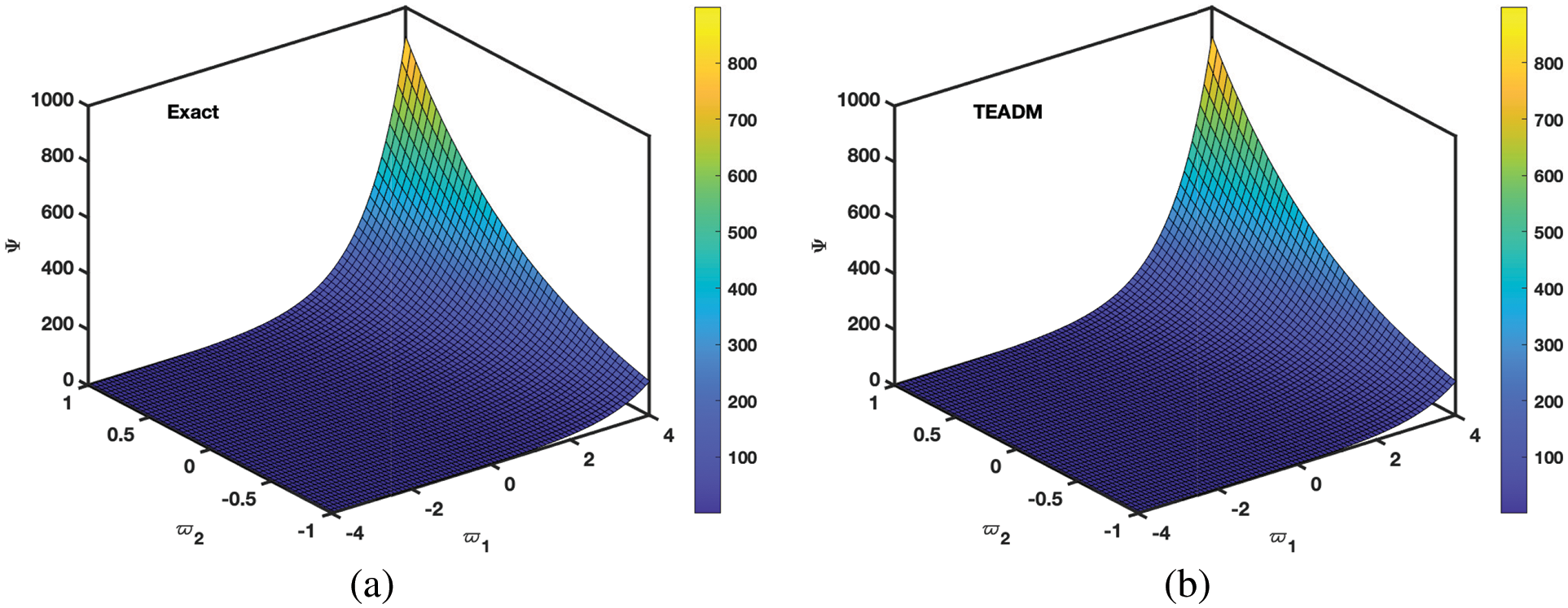
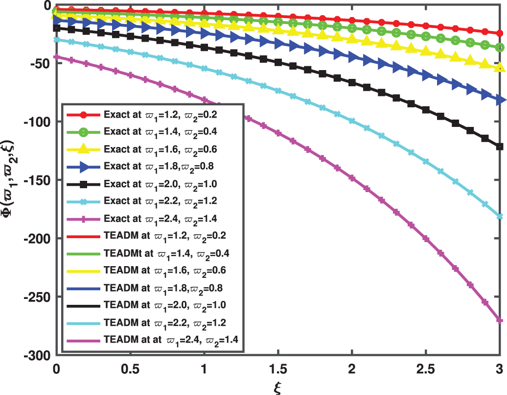
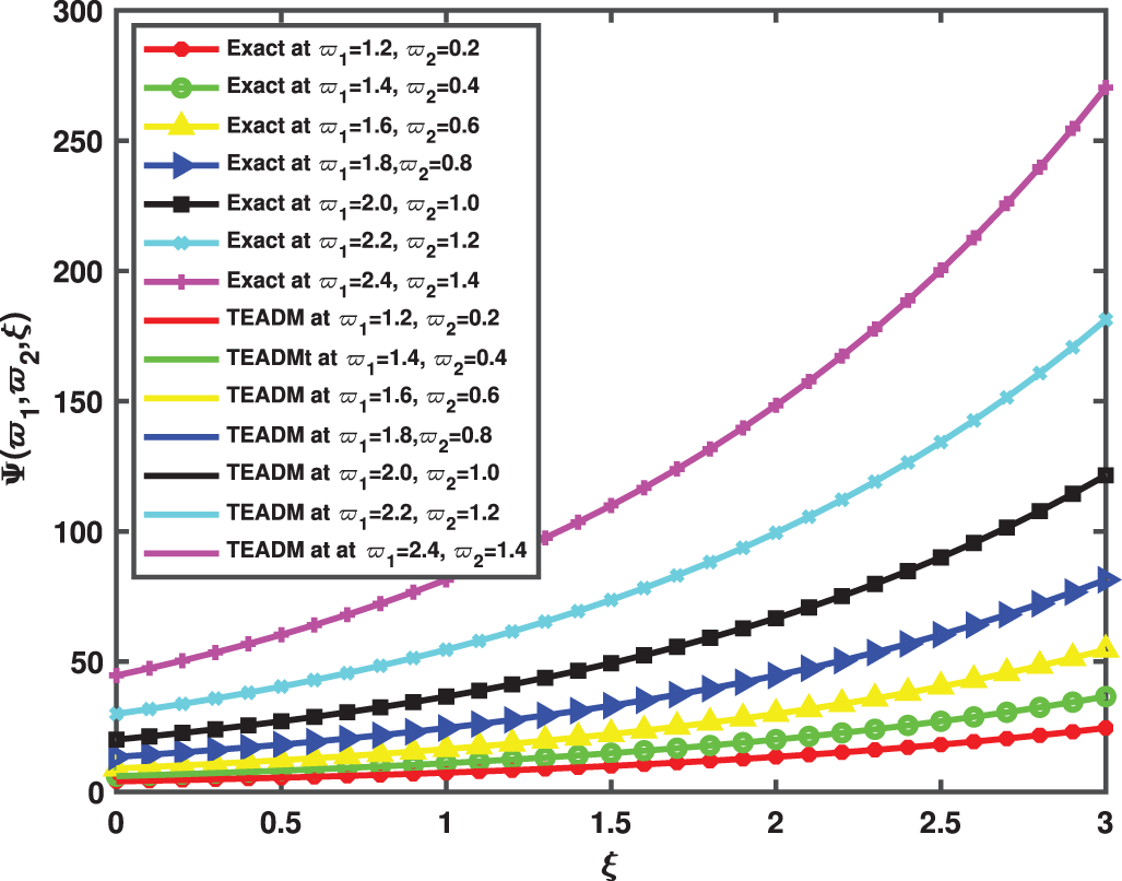
• In Figs. 1 and 2, the 3D surfaces with respect to the Caputo fractional derivative operator at ϕ=1,ρ=0.3 and ℏ=0 are presented. Furthermore, we have demonstrated the graphs of the approximate solutions of functional values Φ(ϖ1,ϖ2,ξ) and Ψ(ϖ1,ϖ2,ξ) of the NSe for Caputo fractional derivative operator, respectively. The Figs. 1a and 2b depicted the approximate solutions, because the TEADM proved to be relatively compelling for solving nonlinear PDEs without linearization, perturbation or discretization. In Figs. 3 and 4, we have described the approximate solution of the problem with respect to the proposed method and exact solution, respectively. One can deduce from the figures that approximate solution approaches the exact solution as the fractional parameter changes from integer-order ϕ=1.
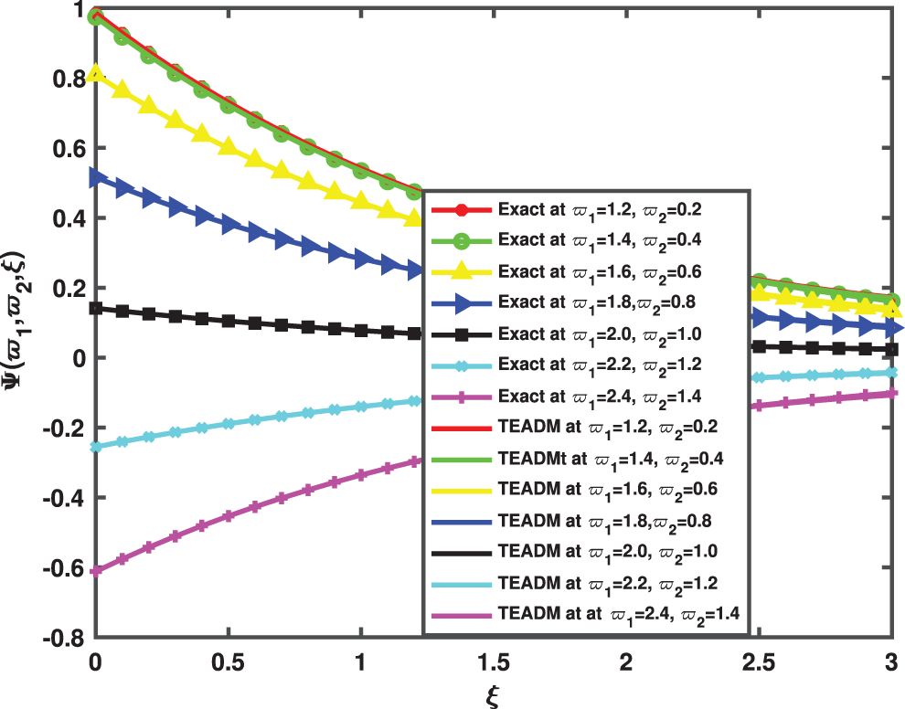
• In Figs. 5–8, the 3D surfaces with respect to the Caputo fractional derivative operator at ϕ=1,ρ=0.3 and ℏ=0 are presented. Furthermore, we have demonstrated the graphs of the approximate solutions of functional values Φ(ϖ1,ϖ2,ξ) and Ψ(ϖ1,ϖ2,ξ) of the NSe for Caputo fractional derivative operator, respectively. The Figs. 5b and 6b depicted the approximate solutions, because the TEADM proved to be relatively promising for solving nonlinear PDEs without linearization, perturbation or discretization. Also, in Fig. 7, the comparison simulation for both Φ and Ψ are also presented to demonstrate the strong correlation between the exact and approximate solution of the proposed technique.
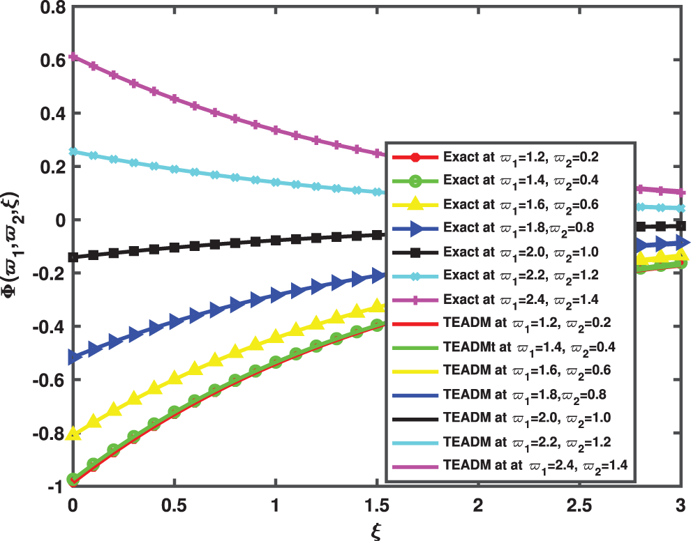
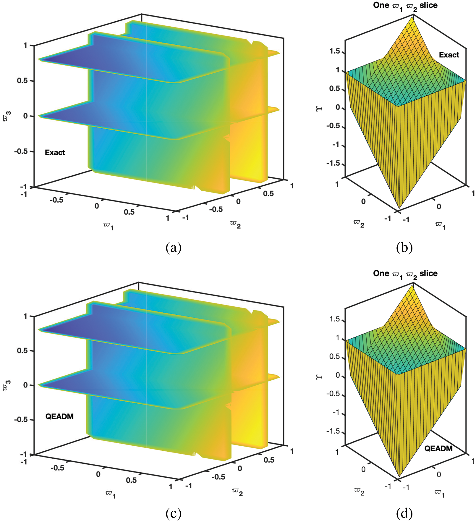
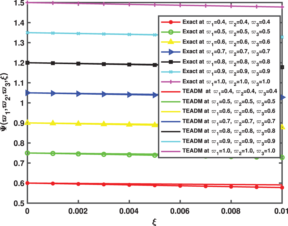
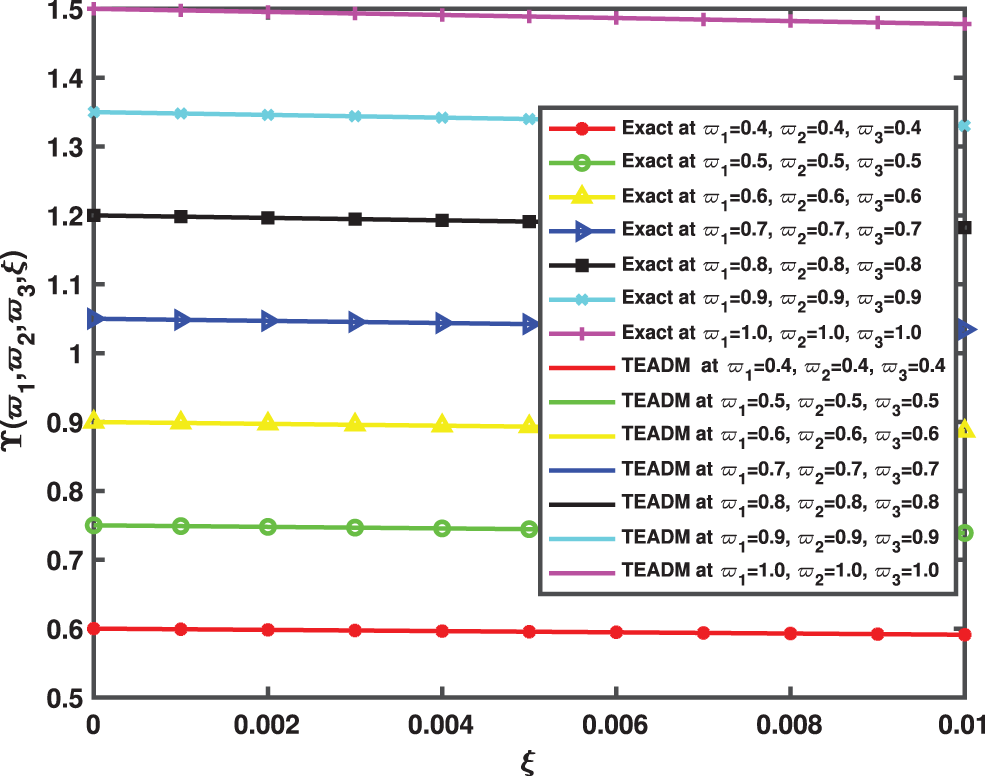
• In Figs. 9–11, we have given the comparison of the exact, ϖ1ϖ2-slice of exact solution given in (35) and in Figs. 12–14, it can be seen that the solution to the problem which is given by (35) with respect to integer-order parameter in the framework of Caputo fractional derivative. Taking into consideration the results of the article, we can view that only a few components of the series derived by the Adomian decomposition method coupled with the Elzaki transform provide the exact solution. Additionally, the comparison simulation for Φ,Ψ and Υ are also presented to demonstrate the strong correlation between the exact and approximate solution by implementing QEADM.
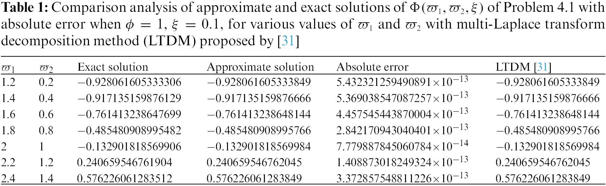
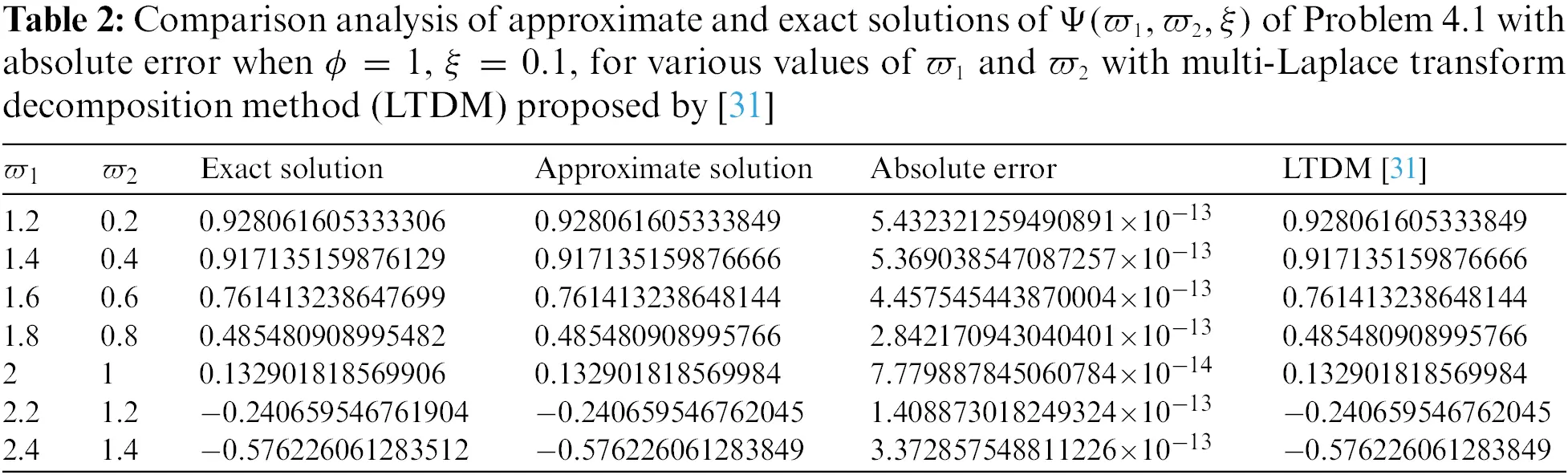
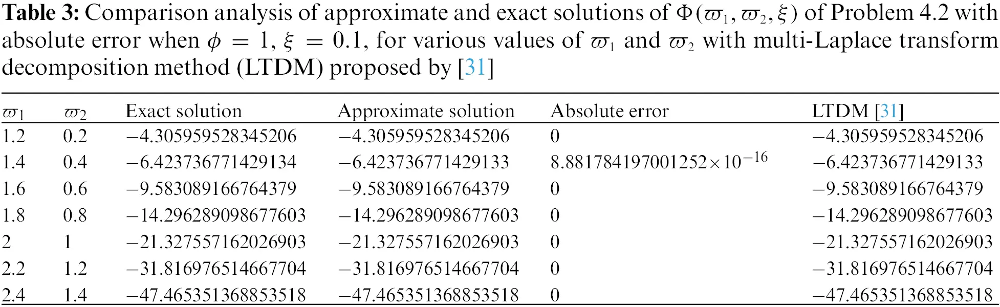
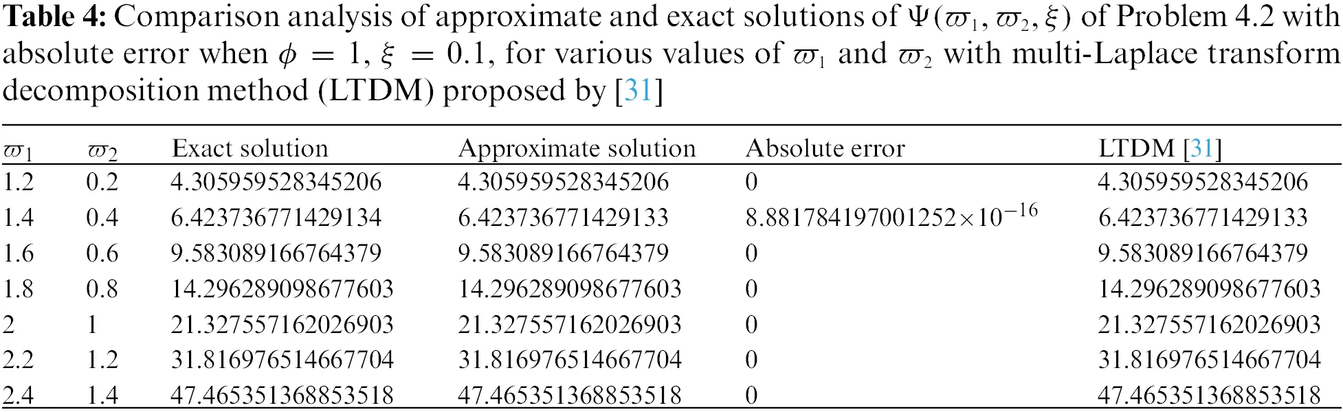
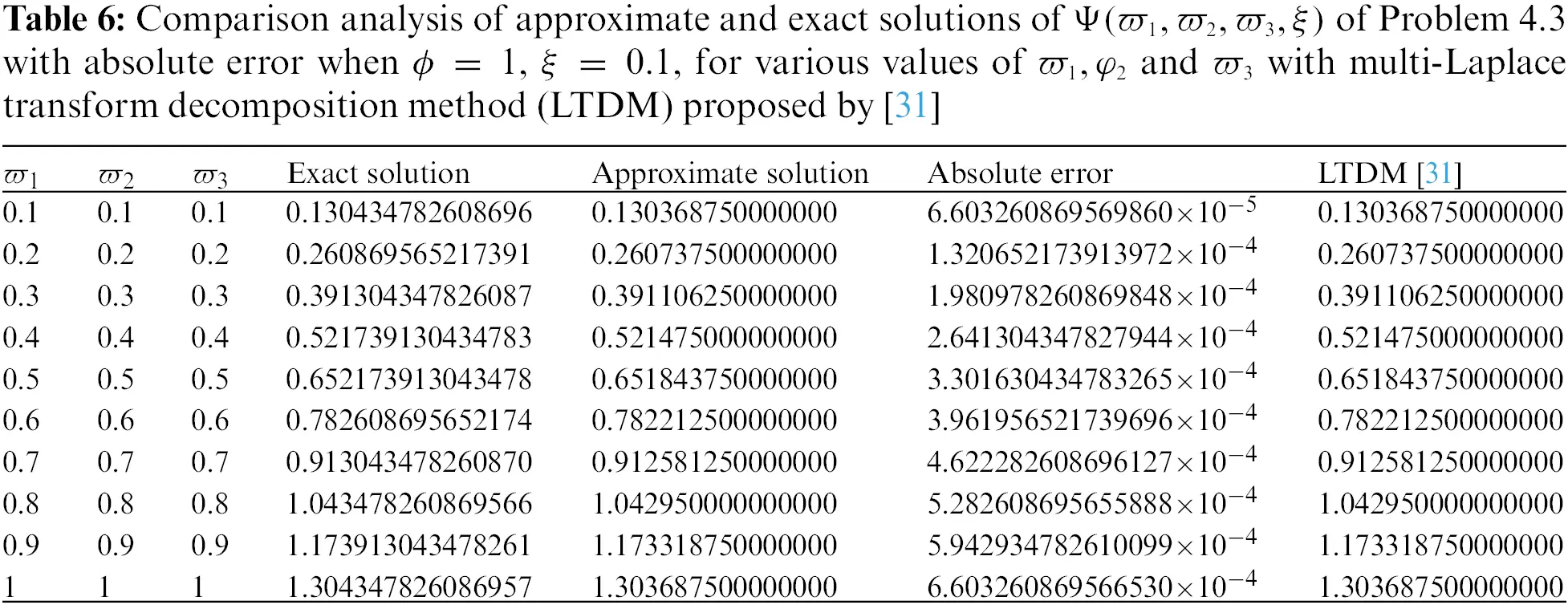
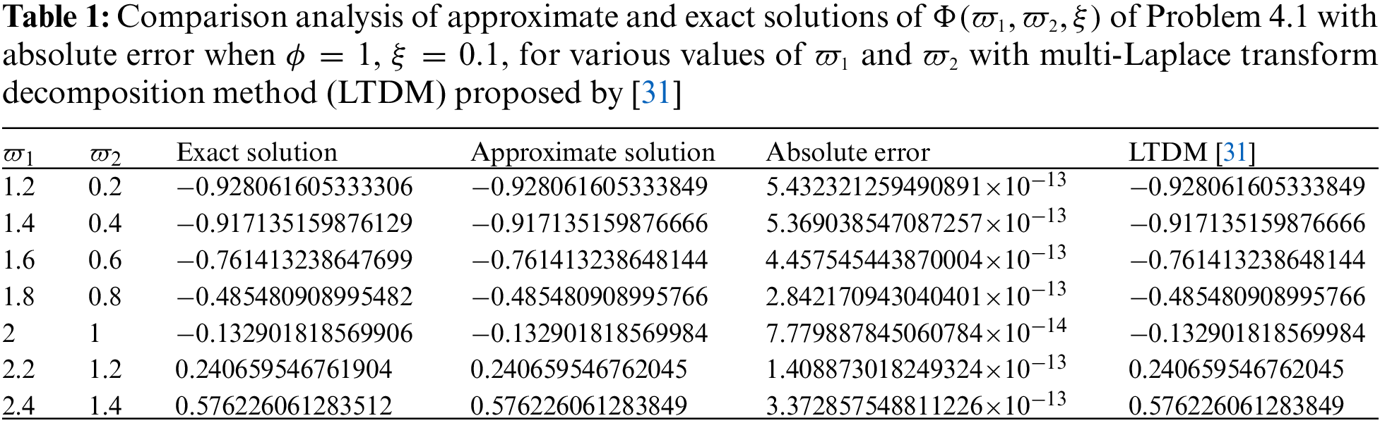
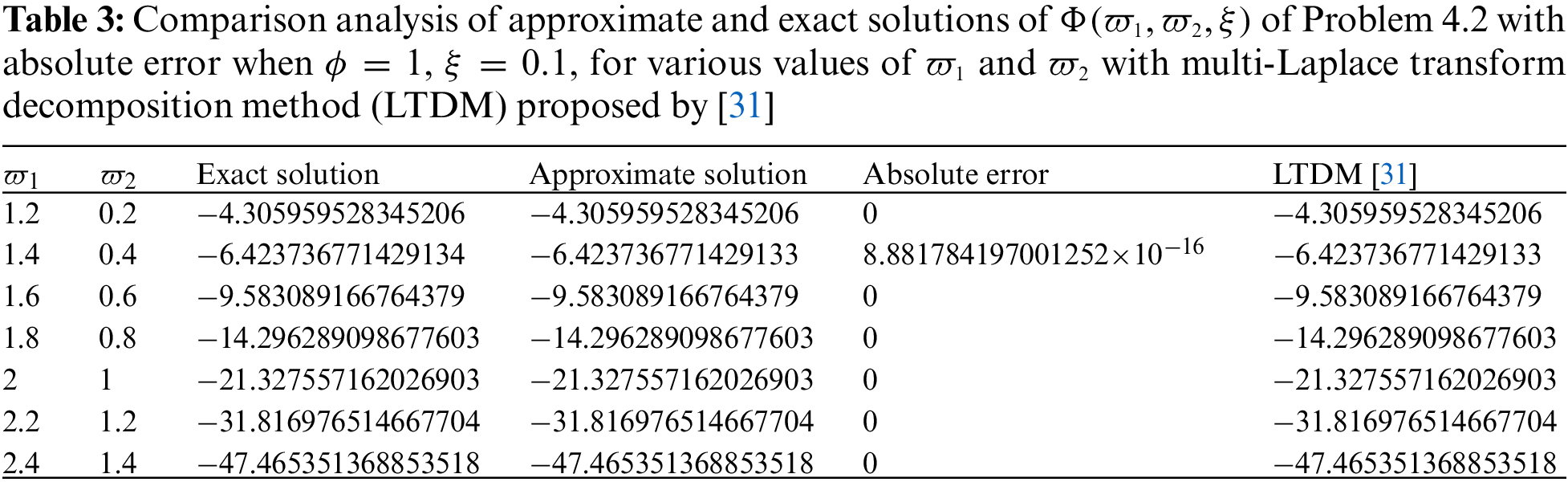
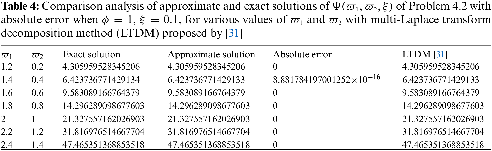
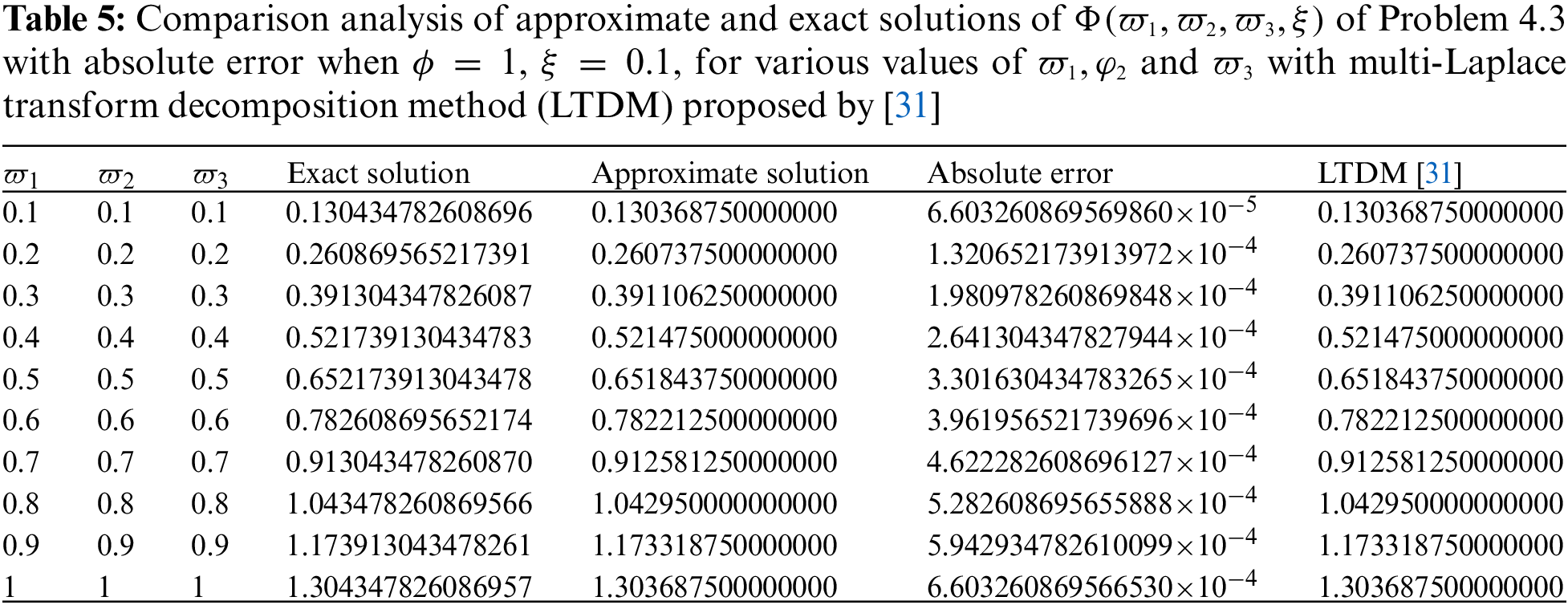
• Tables 1–7 presented a comparison analysis of the findings shown in [31]. The analysis predicts that our projected scheme is close to harmony with the exact solutions.
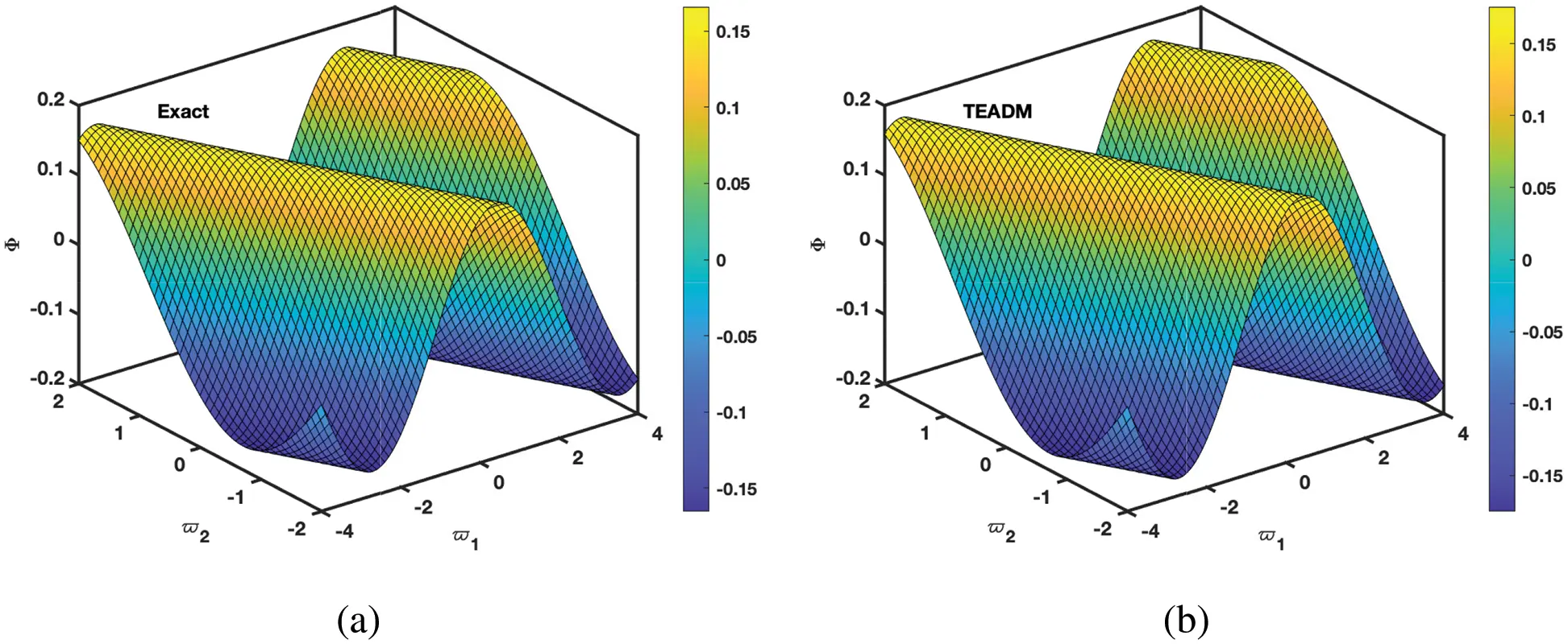
Figure 1: Simulation of the (a) exact and (b) TEADM solutions of Φ(ϖ1,ϖ2,ξ) at ξ=3 of Problem 4.1 when ϕ=1, ρ=0.3, and ℏ=0
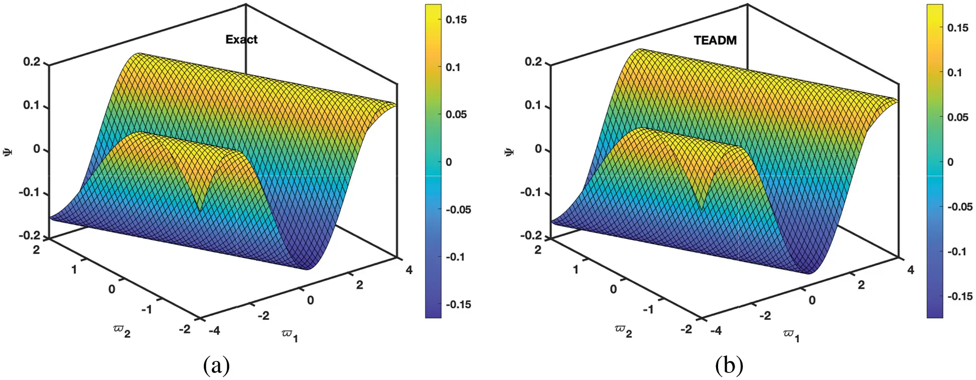
Figure 2: Simulation of the (a) exact and (b) TEADM solutions of Ψ(ϖ1,ϖ2,ξ) of Problem 4.1 with the parameters when ϕ=1, ρ=0.3, and ℏ=0
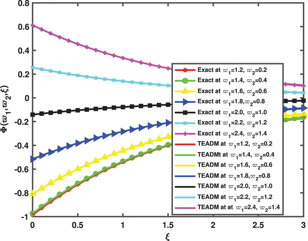
Figure 3: Simulation of the exact and TEADM solutions of Φ(ϖ1,ϖ2,ξ) of Problem 4.1 when ϖ1=1.2 to 2.4, ϖ2=0.2 to 1.4, at ϕ=1, ρ=0.3, and ℏ=0, for various values of ξ
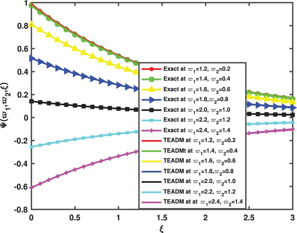
Figure 4: Simulation of the exact and TEADM solutions of Ψ(ϖ1,ϖ2,ξ) of Problem 4.1 when ϖ1=1.2 to 2.4, ϖ2=0.2 to 1.4, at ϕ=1, ρ=0.3, and ℏ=0, for various values of ξ
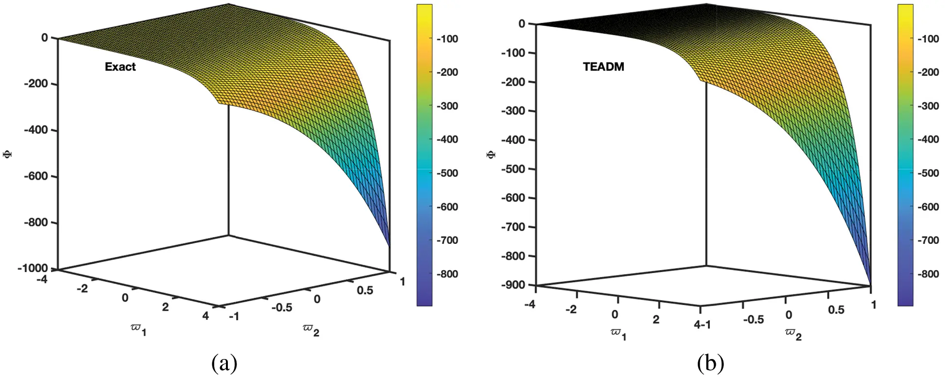
Figure 5: Simulation of the (a) exact and (b) TEADM solutions of Φ(ϖ1,ϖ2,ξ) at ξ=3 of Problem 4.2 with the parameters when ϕ=1, ρ=0.3, and ℏ=0

Figure 6: Simulation of the (a) exact and (b) TEADM solutions of Ψ(ϖ1,ϖ2,ξ) at ξ=3 of Problem 4.2 with the parameters ϕ=1, ρ=0.3, and ℏ=0
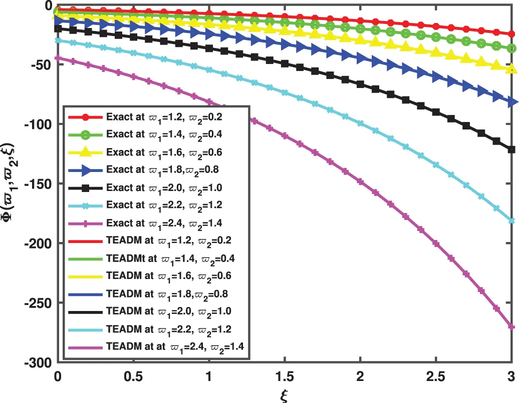
Figure 7: Simulation of the exact and TEADM solutions of Φ(ϖ1,ϖ2,ξ) of Problem 4.2 for ϖ1=1.2 to 2.4, ϖ2=0.2 to 1.4, at ϕ=1, ρ=0.3, and ℏ=0, for various values of ξ
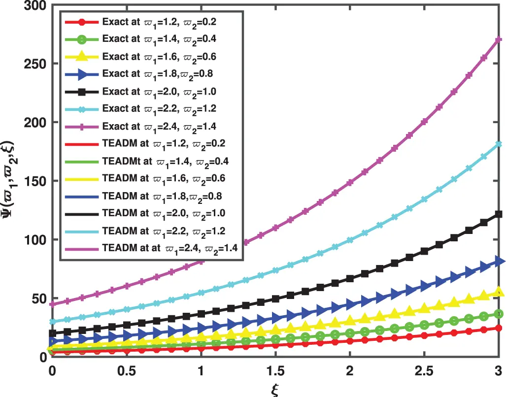
Figure 8: Simulation of the exact and TEADM solutions of Ψ(ϖ1,ϖ2,ξ) of Problem 4.2 when ϖ1=1.2 to 2.4, ϖ2=0.2 to 1.4, at ϕ=1, ρ=0.3, and ℏ=0, for various values of ξ
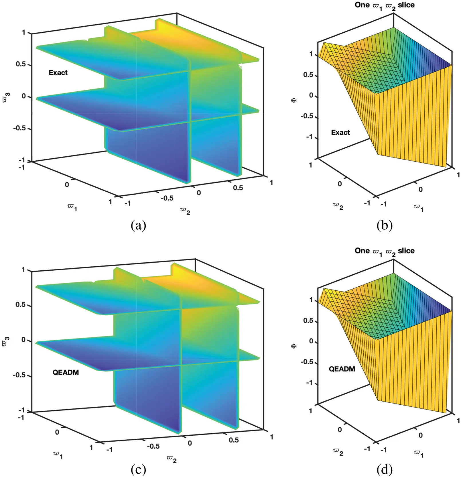
Figure 9: Simulation of the (a) exact solution of Problem 4.3 (b) ϖ1ϖ2-slice of exact solution (c) QEADM solutions of Φ(ϖ1,ϖ2,ϖ3,ξ) of Problem 4.3 when ϕ=1, ρ=0.3, ξ=0.01 and ℏ=0, (d) ϖ1ϖ2-slice of solution of (c)
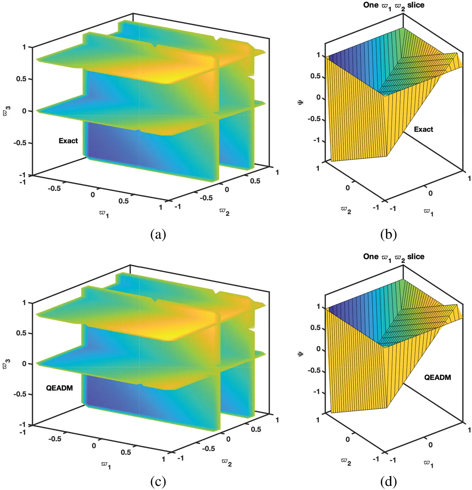
Figure 10: Simulation of the (a) exact solution of Problem 4.3 (b) ϖ1ϖ2-slice of exact solution (c) QEADM solutions of Ψ(ϖ1,ϖ2,ϖ3,ξ) of problem 4.3, at ϕ=1, ρ=0.3, ξ=0.01 and ℏ=0, (d) ϖ1ϖ2-slice of solution of (c)

Figure 11: Simulation of the (a) exact solution of Problem 4.3 (b) ϖ1ϖ2-slice of exact solution (c) QEADM solutions of Υ(ϖ1,ϖ2,ϖ3,ξ) of Problem 4.3 when ϕ=1, ρ=0.3, ξ=0.01 and ℏ=0, (d) ϖ1ϖ2-slice of solution of (c)
Figure 12: Comparison between the exact and QEADM solutions of Φ(ϖ1,ϖ2,ϖ3,ξ) of Problem 4.3 for ϖ1,ϖ2,ϖ3= 0.4 to 1.0 at ϕ=1, ρ=0.3, and ℏ=0, for various values of ξ
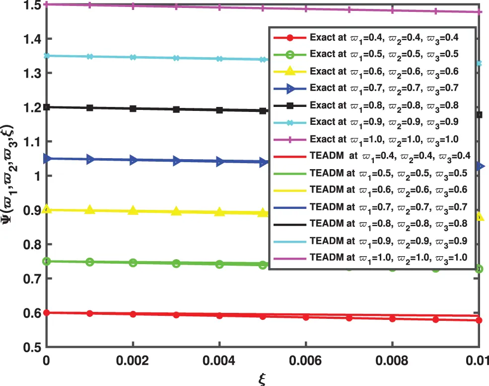
Figure 13: Comparison between the exact and QEADM solutions of Ψ(ϖ1,ϖ2,ϖ3,ξ) of Problem 4.3 for ϖ1,ϖ2,ϖ3= 0.4 to 1.0 at ϕ=1, ρ=0.3, and ℏ=0, for various values of ξ
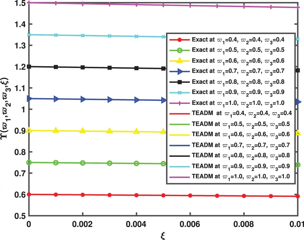
Figure 14: Comparison between the exact and QEADM solutions of Υ(ϖ1,ϖ2,ϖ3,ξ) of Problem 4.3 for ϖ1,ϖ2,ϖ3= 0.4 to 1.0 at ϕ=1, ρ=0.3, and ℏ=0, for various values of ξ


6 Conclusion
The exploration of theoretical models designed to highlight physical process manifestations has indeed drawn researchers’ consideration to their potential to generate provocative results with adequate techniques. In the present investigation, we succeeded in finding analytical solutions to certain nonlinear fractional Navier-Stokes equations employing TEADM and QEADM. More precisely, the hybrid method reported the series of solutions by considering a new iterative approach. The high accuracy of the obtained results with the anticipated technique is expounded in the context of numerical simulation, and the highly complicated behavior has been captured in terms of surface plots. These kinds of investigations can help us examine more intriguing system results, and they widen the window for advancements and reformation in the notion of examining and predicting the more dynamic behavior of the commensurate models that illustrate physical processes. For future research, we extend this study by using the time delays and white noise environments to incorporate the revolutionary techniques of fractional calculus.
Funding Statement: The work was supported by the Natural Science Foundation of China (Grant Nos. 61673169, 11301127, 11701176, 11626101, 11601485).
Conflicts of Interest: The authors declare that they have no conflicts of interest to report regarding the present study.
References
1. Kumar, S., Kumar, A., Samet, B., Gómez-Aguilar, J., Osman, M. (2020). A chaos study of tumor and effector cells in fractional tumor-immune model for cancer treatment. Chaos, Solitons & Fractals, 141(2), 110321. https://doi.org/10.1016/j.chaos.2020.110321 [Google Scholar] [CrossRef]
2. Arqub, O. A., Osman, M. S., Abdel-Aty, A. H., Mohamed, A. B. A., Momani, S. (2020). A numerical algorithm for the solutions of ABC singular lane–emden type models arising in astrophysics using reproducing kernel discretization method. Mathematics, 8(6), 923. https://doi.org/10.3390/math8060923 [Google Scholar] [CrossRef]
3. Ali, K. K., Osman, M. S., Baskonus, H. M., Elazabb, N. S., İlhan, E. (2020). Analytical and numerical study of the HIV-1 infection of CD4+ T-cells conformable fractional mathematical model that causes acquired immunodeficiency syndrome with the effect of antiviral drug therapy. Mathematical Methods in the Applied Sciences. [Google Scholar]
4. Kumar, S., Kumar, R., Osman, M., Samet, B. (2021). A wavelet based numerical scheme for fractional order seir epidemic of measles by using genocchi polynomials. Numerical Methods for Partial Differential Equations, 37(2), 1250–1268. https://doi.org/10.1002/num.22577 [Google Scholar] [CrossRef]
5. Caputo, M. (1969). Elasticita de dissipazione, Zanichelli, Bologna, Italy,(Links). SIAM Journal on Numerical Analysis. [Google Scholar]
6. Shi, L., Tayebi, S., Arqub, O. A., Osman, M., Agarwal, P. et al. (2022). The novel cubic b-spline method for fractional painlevé and bagley-trovik equations in the caputo, caputo-fabrizio, and conformable fractional sense. Alexandria Engineering Journal, 65(6), 413–426. https://doi.org/10.1016/j.aej.2022.09.039 [Google Scholar] [CrossRef]
7. Kilbas, A. A., Marichev, O., Samko, S. (1993). Fractional integrals and derivatives (theory and applications). USA: CRC Press. [Google Scholar]
8. Cuahutenango-Barro, B., Taneco-Hernández, M., Lv, Y. P., Gómez-Aguilar, J., Osman, M. et al. (2021). Analytical solutions of fractional wave equation with memory effect using the fractional derivative with exponential kernel. Results in Physics, 25(1), 104148. https://doi.org/10.1016/j.rinp.2021.104148 [Google Scholar] [CrossRef]
9. Dhawan, S., Machado, J. A. T., Brzeziński, D. W., Osman, M. S. (2021). A chebyshev wavelet collocation method for some types of differential problems. Symmetry, 13(4), 536. https://doi.org/10.3390/sym13040536 [Google Scholar] [CrossRef]
10. Kilbas, A., Trujillo, J. (2002). Differential equations of fractional order: Methods, results and problems. II. Applicable Analysis, 81(2), 435–493. https://doi.org/10.1080/0003681021000022032 [Google Scholar] [CrossRef]
11. Kiryakova, V. S. (2000). Multiple (multiindex) mittag–leffler functions and relations to generalized fractional calculus. Journal of Computational and applied Mathematics, 118(1–2), 241–259. https://doi.org/10.1016/S0377-0427(00)00292-2 [Google Scholar] [CrossRef]
12. Miller, K. S., Ross, B. (1993). An introduction to the fractional calculus and fractional differential equations. New York: Wiley. [Google Scholar]
13. Podlubny, I. (1999). Fractional differential equations, mathematics in science and engineering. San Diego: Academic Press. [Google Scholar]
14. Liouville, J. (1832). Mémoire sur quelques questions de géométrie et de mécanique, et sur un nouveau genre de calcul pour résoudre ces questions. Journal de l’école Polytechnique, tome XIII, XXIe cahier, 1–69. [Google Scholar]
15. Hilfer, R. (2000). Fractional calculus and regular variation in thermodynamics. In: Applications of fractional calculus in physics, pp. 429–463. World Scientific. [Google Scholar]
16. Jafari, H., Jassim, H. K., Baleanu, D., Chu, Y. M. (2021). On the approximate solutions for a system of coupled Korteweg–de Vries equations with local fractional derivative. Fractals, 29(5), 2140012. https://doi.org/10.1142/S0218348X21400120 [Google Scholar] [CrossRef]
17. Rizvi, S., Seadawy, A. R., Ashraf, F., Younis, M., Iqbal, H. et al. (2020). Lump and interaction solutions of a geophysical Korteweg–de Vries equation. Results in Physics, 19(3), 103661. https://doi.org/10.1016/j.rinp.2020.103661 [Google Scholar] [CrossRef]
18. Park, C., Nuruddeen, R., Ali, K. K., Muhammad, L., Osman, M. et al. (2020). Novel hyperbolic and exponential ansatz methods to the fractional fifth-order Korteweg–de Vries equations. Advances in Difference Equations, 2020(1), 1–12. https://doi.org/10.1186/s13662-020-03087-w [Google Scholar] [CrossRef]
19. Cheemaa, N., Seadawy, A. R., Sugati, T. G., Baleanu, D. (2020). Study of the dynamical nonlinear modified Korteweg–de Vries equation arising in plasma physics and its analytical wave solutions. Results in Physics, 19(1), 103480. https://doi.org/10.1016/j.rinp.2020.103480 [Google Scholar] [CrossRef]
20. Khan, H., Shah, R., Kumam, P., Baleanu, D., Arif, M. (2020). Laplace decomposition for solving nonlinear system of fractional order partial differential equations. Advances in Difference Equations, 2020(1), 1–18. https://doi.org/10.1186/s13662-020-02839-y [Google Scholar] [CrossRef]
21. Alderremy, A., Khan, H., Shah, R., Aly, S., Baleanu, D. (2020). The analytical analysis of time-fractional Fornberg–Whitham equations. Mathematics, 8(6), 987. https://doi.org/10.3390/math8060987 [Google Scholar] [CrossRef]
22. Tariq, M., Sahoo, S. K., Ahmad, H., Shaikh, A. A., Kodamasingh, B. et al. (2022). Some integral inequalities via new family of preinvex functions. Mathematical Modelling and Numerical Simulation with Applications, 2(2), 117–126. https://doi.org/10.53391/mmnsa.2022.010 [Google Scholar] [CrossRef]
23. Tariq, M., Ahmad, H., Sahoo, S. K. (2021). The hermite-hadamard type inequality and its estimations via generalized convex functions of raina type. Mathematical Modelling and Numerical Simulation with Applications, 1(1), 32–43. https://doi.org/10.53391/mmnsa.2021.01.004 [Google Scholar] [CrossRef]
24. Inc, M., Khan, M. N., Ahmad, I., Yao, S. W., Ahmad, H. et al. (2020). Analysing time-fractional exotic options via efficient local meshless method. Results in Physics, 19(2), 103385. https://doi.org/10.1016/j.rinp.2020.103385 [Google Scholar] [CrossRef]
25. Yavuz, M. (2019). Characterizations of two different fractional operators without singular kernel. Mathematical Modelling of Natural Phenomena, 14(3), 302. https://doi.org/10.1051/mmnp/2018070 [Google Scholar] [CrossRef]
26. Veeresha, P., Yavuz, M., Baishya, C. (2021). A computational approach for shallow water forced Korteweg–De Vries equation on critical flow over a hole with three fractional operators. An International Journal of Optimization and Control: Theories & Applications, 11(3), 52–67. https://doi.org/10.11121/ijocta.2021.1177 [Google Scholar] [CrossRef]
27. Alderremy, A. A., Elzaki, T. M., Chamekh, M. (2018). New transform iterative method for solving some klein-gordon equations. Results in Physics, 10(3), 655–659. https://doi.org/10.1016/j.rinp.2018.07.004 [Google Scholar] [CrossRef]
28. Navier, C. (1823). Mémoire sur les lois du mouvement des fluides. Mémoires de l’Académie Royale des Sciences de l’Institut de France, 6(1823), 389–440. [Google Scholar]
29. Momani, S., Odibat, Z. (2006). Analytical solution of a time-fractional navier–stokes equation by adomian decomposition method. Applied Mathematics and Computation, 177(2), 488–494. https://doi.org/10.1016/j.amc.2005.11.025 [Google Scholar] [CrossRef]
30. Zhou, Y., Peng, L. (2017). Weak solutions of the time-fractional navier–stokes equations and optimal control. Computers & Mathematics with Applications, 73(6), 1016–1027. https://doi.org/10.1016/j.camwa.2016.07.007 [Google Scholar] [CrossRef]
31. Eltayeb, H., Bachar, I., Abdalla, Y. T. (2020). A note on time-fractional navier–stokes equation and multi-laplace transform decomposition method. Advances in Difference Equations, 2020(1), 1–19. https://doi.org/10.1186/s13662-020-02981-7 [Google Scholar] [CrossRef]
32. Shah, R., Khan, H., Baleanu, D., Kumam, P., Arif, M. (2020). The analytical investigation of time-fractional multi-dimensional navier–stokes equation. Alexandria Engineering Journal, 59(5), 2941–2956. https://doi.org/10.1016/j.aej.2020.03.029 [Google Scholar] [CrossRef]
33. Singh, B. K., Kumar, P. (2018). FRDTM for numerical simulation of multi-dimensional, time-fractional model of Navier–Stokes equation. Ain Shams Engineering Journal, 9(4), 827–834. https://doi.org/10.1016/j.asej.2016.04.009 [Google Scholar] [CrossRef]
34. Khan, H., Khan, A., Kumam, P., Baleanu, D., Arif, M. et al. (2020). An approximate analytical solution of the navier–stokes equations within caputo operator and elzaki transform decomposition method. Advances in Difference Equations, 2020(1), 1–23. [Google Scholar]
35. Elzaki, T. M. (2011). The new integral transform elzaki transform. Global Journal of Pure and Applied Mathematics, 7(1), 57–64. [Google Scholar]
36. Elzaki, T. M. (2011). Application of new transform “elzaki transform” to partial differential equations. Global Journal of Pure and Applied Mathematics, 7(1), 65–70. [Google Scholar]
37. Adomian, G. (1994). Solution of physical problems by decomposition. Computers & Mathematics with Applications, 27(9–10), 145–154. https://doi.org/10.1016/0898-1221(94)90132-5 [Google Scholar] [CrossRef]
38. Adomian, G. (1988). A review of the decomposition method in applied mathematics. Journal of Mathematical Analysis and Applications, 135(2), 501–544. https://doi.org/10.1016/0022-247X(88)90170-9 [Google Scholar] [CrossRef]
39. Elzaki, T. M. (2011). On the connections between laplace and elzaki transforms. Advances in Theoretical and Applied Mathematics, 6(1), 1–11. [Google Scholar]
40. Elzaki, T. M., Ezaki, S. M. (2011). On the elzaki transform and ordinary differential equation with variable coefficients. Advances in Theoretical and Applied Mathematics, 6(1), 41–46. [Google Scholar]
41. Atluri, S. N., Shen, S. (2002). The meshless local petrov-galerkin (MLPG) method (Ph.D. Thesis). Crest, USA. [Google Scholar]

 Submit a Paper
 Propose a Special lssue
 Open Access
 View Full Text
 Download PDF


 Copyright © 2023 The Author(s). Published by Tech Science Press.
 Downloads
 Citation Tools