
 Submit a Paper
 Propose a Special lssue
 Open Access
ARTICLE

A Study on the Nonlinear Caputo-Type Snakebite Envenoming Model with Memory
1 Department of Mathematics, National Institute of Technology Puducherry, Karaikal, 609609, India
2 Department of Mathematics, Faculty of Arts and Sciences, Ondokuz Mayis University, Atakum, Samsun, 55200, Turkey
3 Department of Mathematics, Cankaya University, Ankara, 06530, Turkey
4 Institute of Space Sciences, Magurele, Bucharest, R76900, Romania
5 Department of Computer Science and Mathematics, Lebanese American University, Beirut, 11022801, Lebanon
* Corresponding Author: Pushpendra Kumar. Email:
Computer Modeling in Engineering & Sciences 2023, 136(3), 2487-2506. https://doi.org/10.32604/cmes.2023.026009
Received 09 August 2022; Accepted 10 November 2022; Issue published 09 March 2023
 View Full Text
 Download PDF
Abstract
In this article, we introduce a nonlinear Caputo-type snakebite envenoming model with memory. The well-known Caputo fractional derivative is used to generalize the previously presented integer-order model into a fractional-order sense. The numerical solution of the model is derived from a novel implementation of a finite-difference predictor-corrector (L1-PC) scheme with error estimation and stability analysis. The proof of the existence and positivity of the solution is given by using the fixed point theory. From the necessary simulations, we justify that the first-time implementation of the proposed method on an epidemic model shows that the scheme is fully suitable and time-efficient for solving epidemic models. This work aims to show the novel application of the given scheme as well as to check how the proposed snakebite envenoming model behaves in the presence of the Caputo fractional derivative, including memory effects.Keywords
Nowadays, fractional calculus [1–3] is being applied to solve various real-world problems in terms of mathematical modeling. Different fractional derivatives [4] have been successfully used to model various problems. More specifically, several deadly epidemics have been modeled by using mathematical models in a fractional-order sense. It is a well-known fact that the fractional-order operators are non-local in nature and may be more effective for modeling history (memory)-dependent systems. Moreover, a fractional order can be fixed as any positive real number that better fits a real-data. So, by using such an operator, an accurate adjustment can be done in a model to fit with real data for better predicting the outbreaks of an epidemic. Recently, several applications of fractional derivatives have been recorded in epidemiology. In [5–7], the authors have studied the dynamics of the COVID-19 epidemic by using fractional-order mathematical models. In [8], the authors used non-singular Caputo-Fabrizio and Atangana-Baleanu fractional derivatives to study the dynamical nature of a malaria epidemic model. Kumar et al. in [9] have solved canine distemper virus and rabies epidemic models in the sense of generalized Caputo derivative. Kumar et al. [10] defined two different types of fractional-order models to study the dynamics of mosaic disease. A novel application of the generalized Caputo derivative in environmental infection dynamics can be seen in [11]. Sinan et al. [12] proposed the mathematical modeling of typhoid fever in terms of fractional derivatives. In [13], some novel analyses on the numerical modeling of biological systems using fractional derivatives have been given. Rihan et al. [14] studied fractional-order predator-prey models, including delay with Holling type-II functional response. In [15], some novel applications of delay differential equations were proposed. Work on the application of fractional derivatives in ecology and psychology can be understood from [16,17], respectively.
To analyze the various types of fractional-order systems, several computational schemes have been proposed by researchers. Odibat et al. [18] derived a new generalized form of the predictor-corrector (PC) scheme to investigate fractional initial value problems. Kumar et al. [19] introduced a new method to simulate fractional-order systems with various examples. In [20], the PC method was derived to simulate delay fractional differential equations. A modified form of the PC scheme in terms of the generalized Caputo derivative to solve delay-type systems has been introduced in reference [21]. Odibat et al. [22] have derived the generalized differential transform method for solving fractional impulsive differential equations. In [23], some computational schemes to solve delayed parabolic and time-fractional partial differential equations have been proposed. Shah et al. [24] simulated the dynamics of some important fractional order differential equations. In [25], some novel analyses of the Cauchy-type fractional-order dynamical system in terms of piecewise equations have been given. Some more applications of fractional derivatives can be seen in [26–28].
Jhinga et al. [29] introduced a novel finite-difference predictor-corrector (L1-PC) scheme to solve fractional-order systems in the sense of the Caputo derivative. That L1-PC scheme is not yet applied to any epidemic model to check how it will work and show the disease dynamics. In this paper, we fill this research gap by implementing the given L1-PC method on a Caputo-type snakebite envenoming (SBE) mathematical model, which was previously proposed in the integer-order sense in reference [30]. Currently, SBE is a deathly neglected disease, mainly in developing nations. The World Health Organization (WHO) recognized SBE as a fatal disease that generally results from the injection of a combination of various toxins (venom) following a venomous snakebite. Mainly poor, rural societies in tropical and subtropical nations all over the world are typically affected by SBE, which is a big threat to the health and well-being of about 5.8 billion population [31]. More information on SBE can be collected from the references [32–34]. To date, only a few research studies have gone into the mathematical modeling of SBE. In [35], the authors introduced a model using the law of mass action to analyze snakebite incidence. In [36], a mathematical model considering the socio-demographic components that influence the death risk from SBE in India was proposed.
The motivation of this study is to justify the application of the aforementioned L1-PC scheme in epidemiology by solving a mathematical model of SBE. Also, the aim is to check how the proposed SBE model will behave in the presence of the Caputo fractional derivative, which is a non-local differential operator that allows memory effects in the system. The given study is designed using the following systems: Section 2 recalls some preliminaries of fractional calculus. The description of the considered model of SBE in terms of the Caputo derivative is given in Section 3. The necessary numerical analysis, like the solution algorithm, error estimation, and method stability, is performed in Section 4. A brief discussion of the proposed methodology, its novelty, and outputs is given in Section 5 with supporting conclusions.
Here we recall some preliminaries of fractional calculus.
Definition 1. A real function
a)
b)
Definition 2. [2] The Riemann-Liouville fractional integral of
Definition 3. [2] The Caputo fractional derivative of
Theorem 1. [37] Consider the function f such that f and
Therefore, from Theorem 1, we say that if
Lemma 1. [38] Let
where
with the same initial constraints, where j is a positive integer. If
Here we introduce the generalized form of the previously published integer-order model [30] into Caputo-type fractional-order sense (
The total snake population is defined by
where,
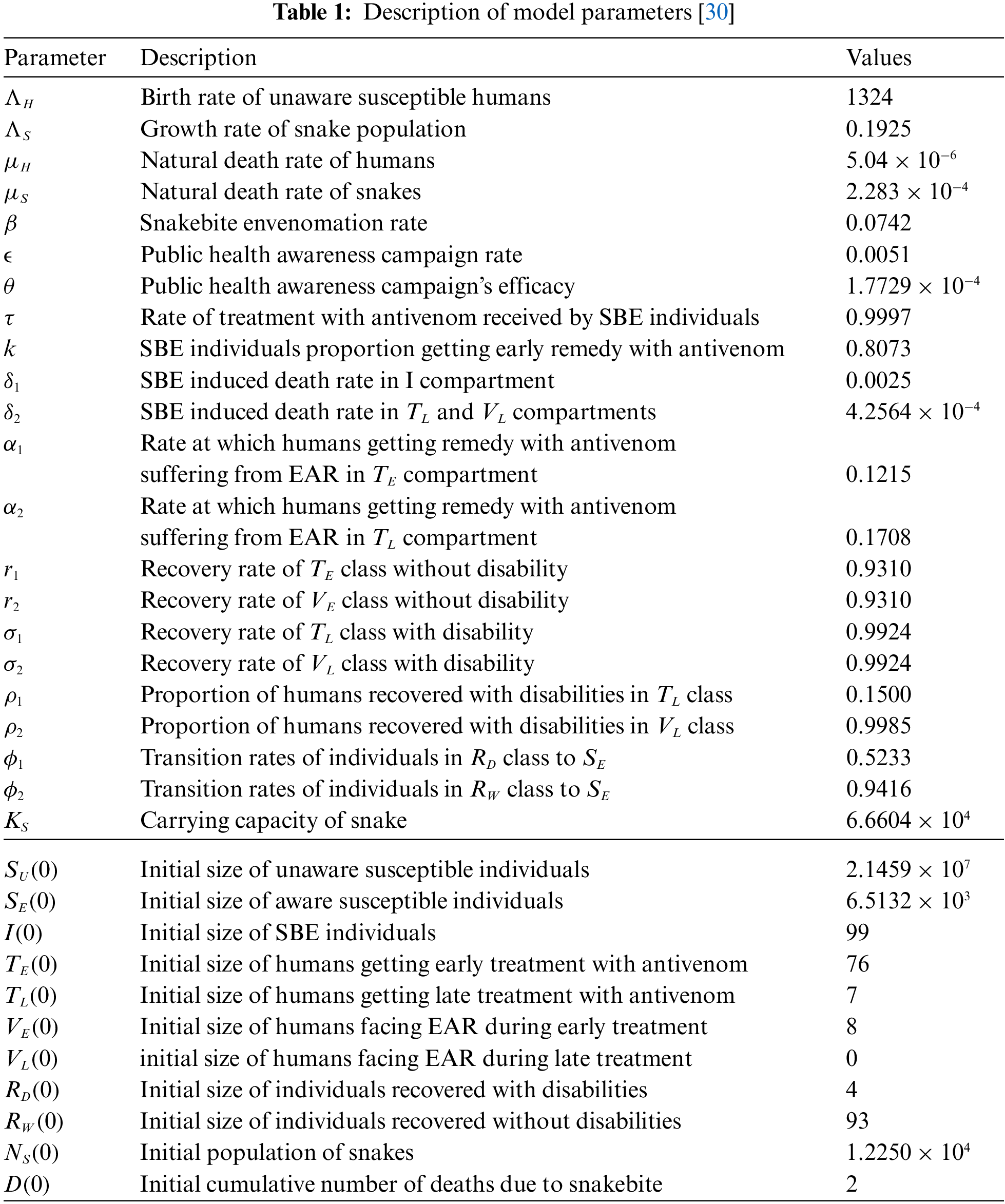
The definitions of the model parameters alongwith their numerical values are given in Table 1.
Theorem 2. There exists a unique solution for the model (3) and (4) which belongs to
Proof. By using the Theorem 3.1 and Remark 3.2 of [39], the global existence of the unique solution can easily be proved. Now to prove the non-negativity of the solution, let us write the following auxiliary system of fractional differential equations:
with
by continuity of
Now before performing the further numerical simulations on the proposed fractional-order model (3), we rewrite the model into a compact form by representing it in terms of an initial value problem, defined as follows:
Let us consider
By using (6), we have
where
4 Numerical Analysis on the Model
In this section, we perform the necessary numerical simulations (solution derivation, error estimation and stability) to derive the solution of the proposed fractional-order model (3) by using the L1-predictor-corrector scheme [29].
Consider the above given initial value problem (IVP) for
where
4.1 Derivation of the Solution
According to the L1-PC method, the Caputo fractional derivative is numerically defined by
where,
We approximate
where
(11) can be rewritten as
After rewriting the terms (12), we get the following from:
Substituting
in (12), we get
Define
Remark that
•
•
•
Given Eqs. (14) and (15), the following form can be obtained:
We can see that Eq. (16) is of the form
and
Hence using the scheme of the DGJ method gives approximate value of
The three term approximation of
where
Using the above given methodology, the approximation equations of the proposed model (3) in terms of L1-PC method are derived as follows:
where,
and
The above given algorithm is coded in Mathematica and the bunch of Figs. 1 and 2 plotted to explore the outputs of the scheme at various fractional-order values. From the Figs. 1c–1f, we identify when the fractional order decreases, the population of the SBE humans;
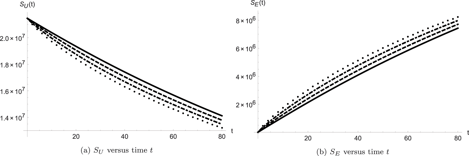
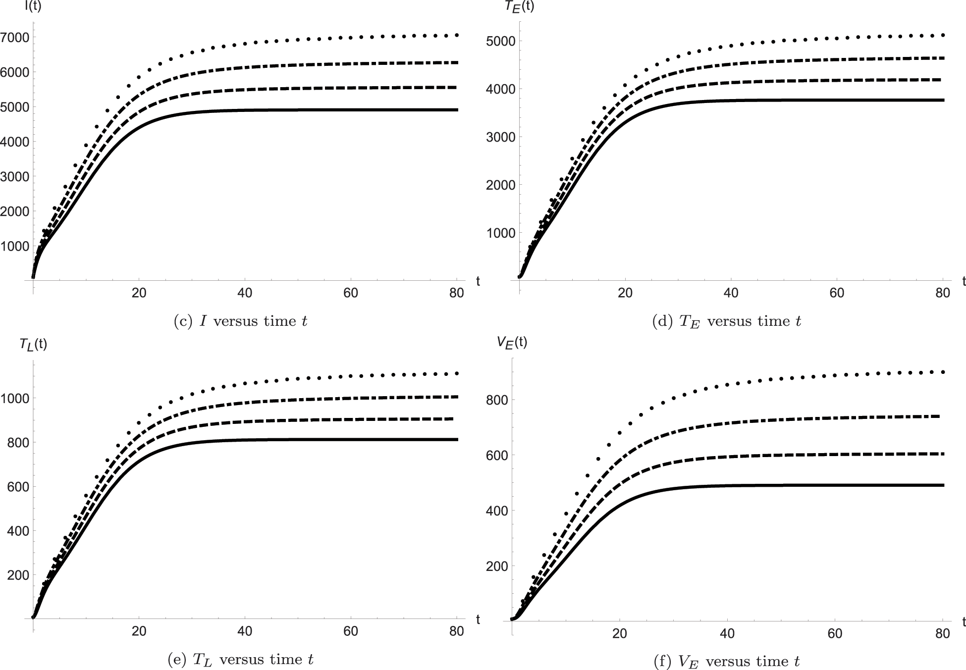
Figure 1: Dynamics of the model classes
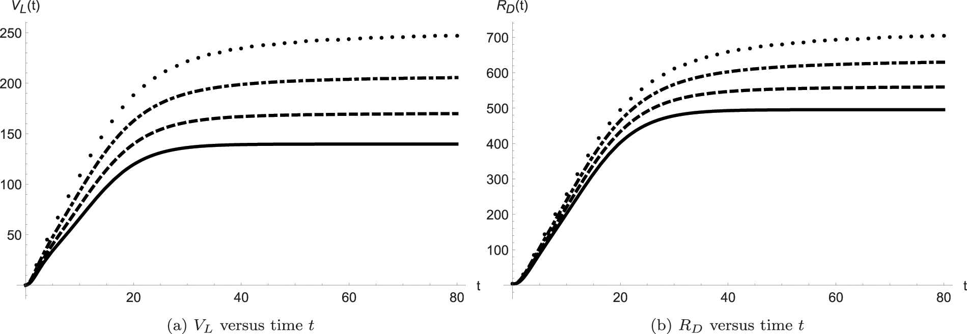
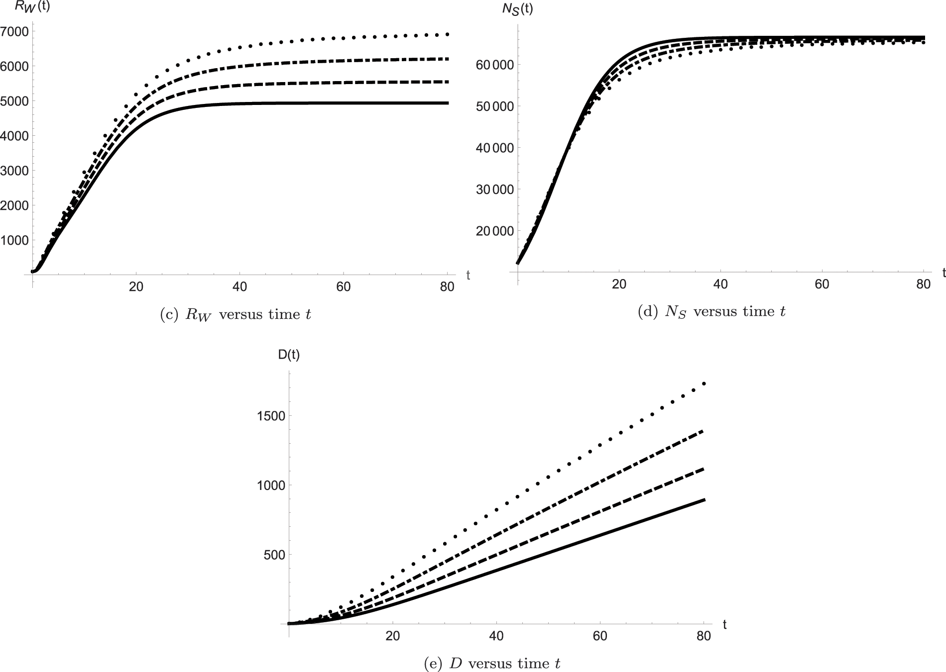
Figure 2: Dynamics of the model classes
The brief analysis on the error estimation of L1-PC scheme has been given in the studies [29,40,41] and now investigated below. The error estimate is given by
here C is a positive constant depends on
Derive
In view of (21)
To derive the error estimation, we will use the lemmas given below:
Lemma 2. [42] For
Lemma 3. [29] Consider
where
Lemma 4. [29] Consider
where
Theorem 3. Consider
where
Proof. Let
Further observe that
Using Lemma 4 in Eq. (25), we get
Therefore
where
The behaviour of the absolute remainder error is plotted in the bundle of Figs. 3 and 4 at the previously used fractional-order values
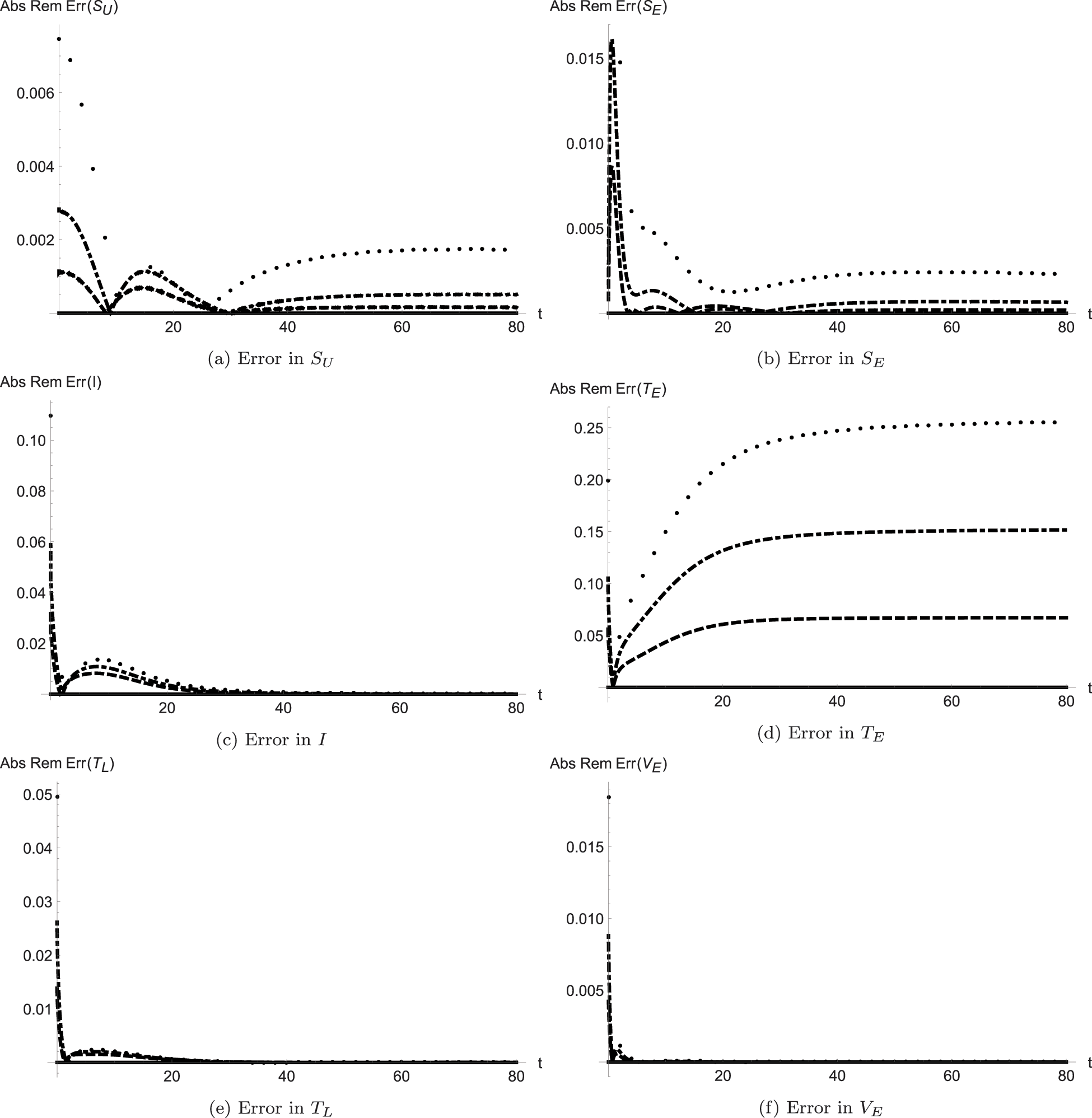
Figure 3: Absolute remainder error in the solution of the model classes
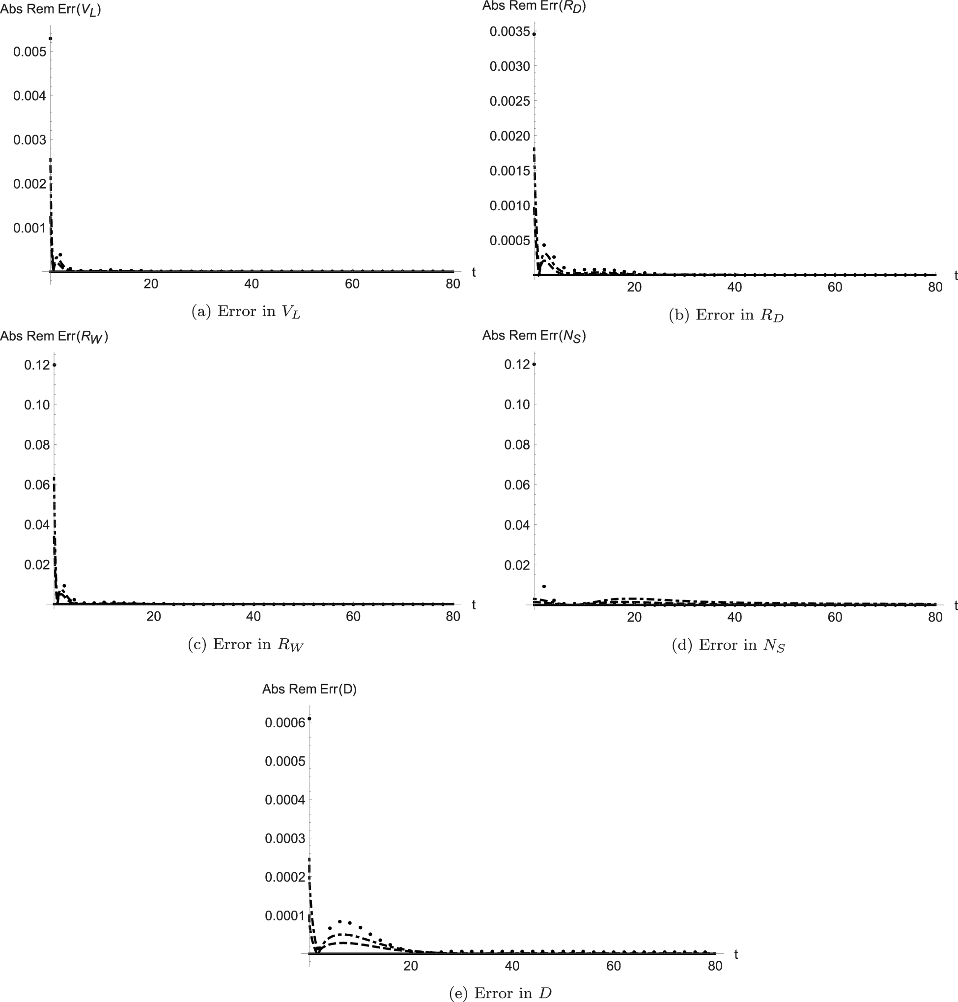
Figure 4: Absolute remainder error in the solution of the model classes
The term stability means that small deviations in the initial values do not make the big changes in the numerical solutions. Consider that
here h is the step size given in Eq. (9).
Theorem 4. Suppose
Proof. We have to prove that
Denote by
Further observe that
Using discrete form of Gronwalls inequality and Eq. (15), we obtain
where c is a constant and
Using (27) and (28) in (26), we get
where C is a constant.
In this research work, we have performed a novel implementation of a finite-difference predictor-corrector scheme on a fractional-order nonlinear snakebite envenoming model in terms of the Caputo fractional derivative. The numerical solution of the model has been plotted by using several graphs to justify the behavior of the model at various fractional-order values. The analysis related to the error estimation and stability of the scheme has also been derived from exploring method’s accuracy. In the error estimation, the fractional order
Funding Statement: The authors received no specific funding for this study.
Author Contributions: P. Kumar: Conceptualization, Visualization, Resources, Formal analysis, Investigation, Writing-original draft. V.S. Erturk: Conceptualization, Investigation, Visualization, Software, Writing-review & editing. V. Govindaraj: Investigation, Resources, Formal analysis, Writing-review & editing. D. Baleanu: Investigation, Resources, Formal analysis, Writing-review & editing.
Availability of Data and Materials: The data used in this research is available/mentioned in the manuscript.
Conflicts of Interest: The authors declare that they have no conflicts of interest to report regarding the present study.
References
1. Kilbas, A., Srivastava, H. M., Trujillo, J. J. (2006). Theory and applications of fractional differential equations. Netherlands: Elsevier Science. [Google Scholar]
2. Podlubny, I. (1998). Fractional differential equations: An introduction to fractional derivatives, fractional differential equations, to methods of their solution and some of their applications. USA: Elsevier. [Google Scholar]
3. Oldham, K., Spanier, J. (1974). The fractional calculus theory and applications of differentiation and integration to arbitrary order. USA: Elsevier. [Google Scholar]
4. Caputo, M., Fabrizio, M. (2015). A new definition of fractional derivative without singular kernel. Progress in Fractional Differentiation & Applications, 1(2), 73–85. [Google Scholar]
5. Erturk, V. S., Kumar, P. (2020). Solution of a COVID-19 model via new generalized caputo-type fractional derivatives. Chaos, Solitons & Fractals, 139, 110280. https://doi.org/10.1016/j.chaos.2020.110280 [Google Scholar] [PubMed] [CrossRef]
6. Ahmad, S., Ullah, A., Al-Mdallal, Q. M., Khan, H., Shah, K. et al. (2020). Fractional order mathematical modeling of COVID-19 transmission. Chaos, Solitons & Fractals, 139, 110256. https://doi.org/10.1016/j.chaos.2020.110256 [Google Scholar] [PubMed] [CrossRef]
7. Higazy, M. (2020). Novel fractional order SIDARTHE mathematical model of COVID-19 pandemic. Chaos, Solitons & Fractals, 138, 110007. https://doi.org/10.1016/j.chaos.2020.110007 [Google Scholar] [PubMed] [CrossRef]
8. Abboubakar, H., Kumar, P., Rangaig, N. A., Kumar, S. (2020). A malaria model with Caputo-Fabrizio and Atangana-Baleanu derivatives. International Journal of Modeling, Simulation, and Scientific Computing, 12(2), 2150013. https://doi.org/10.1142/S1793962321500136 [Google Scholar] [CrossRef]
9. Kumar, P., Erturk, V. S., Yusuf, A., Nisar, K. S., Abdelwahab, S. F. (2021). A study on canine distemper virus (CDV) and rabies epidemics in the red fox population via fractional derivatives. Results in Physics, 25, 104281. https://doi.org/10.1016/j.rinp.2021.104281 [Google Scholar] [CrossRef]
10. Kumar, P., Erturk, V. S., Almusawa, H. (2021). Mathematical structure of mosaic disease using microbial biostimulants via Caputo and Atangana-Baleanu derivatives. Results in Physics, 24, 104186. https://doi.org/10.1016/j.rinp.2021.104186 [Google Scholar] [CrossRef]
11. Kumar, P., Erturk, V. S. (2021). Environmental persistence influences infection dynamics for a butterfly pathogen via new generalised Caputo type fractional derivative. Chaos, Solitons & Fractals, 144, 110672. https://doi.org/10.1016/j.chaos.2021.110672 [Google Scholar] [CrossRef]
12. Sinan, M., Shah, K., Kumam, P., Mahariq, I., Ansari, K. J. et al. (2022). Fractional order mathematical modeling of typhoid fever disease. Results in Physics, 32, 105044. https://doi.org/10.1016/j.rinp.2021.105044 [Google Scholar] [CrossRef]
13. Rihan, F. A. (2013). Numerical modeling of fractional-order biological systems. Abstract and Applied Analysis, 2013. https://doi.org/10.1155/2013/816803 [Google Scholar] [CrossRef]
14. Rihan, F. A., Lakshmanan, S., Hashish, A. H., Rakkiyappan, R., Ahmed, E. (2015). Fractional-order delayed predator–prey systems with holling type-II functional response. Nonlinear Dynamics, 80(1), 777–789. https://doi.org/10.1007/s11071-015-1905-8 [Google Scholar] [CrossRef]
15. Rihan, F. A. (2021). Delay differential equations and applications to biology. Singapore: Springer. [Google Scholar]
16. Kumar, P., Erturk, V. S., Banerjee, R., Yavuz, M., Govindaraj, V. (2021). Fractional modeling of plankton-oxygen dynamics under climate change by the application of a recent numerical algorithm. Physica Scripta, 96(12), 124044. https://doi.org/10.1088/1402-4896/ac2da7 [Google Scholar] [CrossRef]
17. Kumar, P., Erturk, V. S., Murillo-Arcila, M. (2021). A complex fractional mathematical modeling for the love story of Layla and Majnun. Chaos, Solitons & Fractals, 150, 111091. https://doi.org/10.1016/j.chaos.2021.111091 [Google Scholar] [CrossRef]
18. Odibat, Z. Baleanu, D. (2020). Numerical simulation of initial value problems with generalized caputo-type fractional derivatives. Applied Numerical Mathematics, 156, 94–105. https://doi.org/10.1016/j.apnum.2020.04.015 [Google Scholar] [CrossRef]
19. Kumar, P., Erturk, V. S., Kumar, A. (2021). A new technique to solve generalized Caputo type fractional differential equations with the example of computer virus model. Journal of Mathematical Extension, 15, 1–23. [Google Scholar]
20. Bhalekar, S. Daftardar-Gejji, V. (2011). A predictor-corrector scheme for solving nonlinear delay differential equations of fractional order. Journal of Fractional Calculus and Applications, 1(5), 1–9. [Google Scholar]
21. Odibat, Z., Erturk, V. S., Kumar, P., Govindaraj, V. (2021). Dynamics of generalized Caputo type delay fractional differential equations using a modified predictor-corrector scheme. Physica Scripta, 96(12), 125213. https://doi.org/10.1088/1402-4896/ac2085 [Google Scholar] [CrossRef]
22. Odibat, Z., Erturk, V. S., Kumar, P., Ben Makhlouf, A., Govindaraj, V. (2022). An implementation of the generalized differential transform scheme for simulating impulsive fractional differential equations. Mathematical Problems in Engineering, 2022. https://doi.org/10.1155/2022/8280203 [Google Scholar] [CrossRef]
23. Rihan, F. A. (2010). Computational methods for delay parabolic and time-fractional partial differential equations. Numerical Methods for Partial Differential Equations, 26(6), 1556–1571. https://doi.org/10.1002/num.20504 [Google Scholar] [CrossRef]
24. Shah, K., Arfan, M., Ullah, A., Al-Mdallal, Q., Ansari, K. J. et al. (2022). Computational study on the dynamics of fractional order differential equations with applications. Chaos, Solitons & Fractals, 157, 111955. https://doi.org/10.1016/j.chaos.2022.111955 [Google Scholar] [CrossRef]
25. Shah, K., Abdeljawad, T., Ali, A. (2022). Mathematical analysis of the Cauchy type dynamical system under piecewise equations with caputo fractional derivative. Chaos, Solitons & Fractals, 161, 112356. https://doi.org/10.1016/j.chaos.2022.112356 [Google Scholar] [CrossRef]
26. Amin, M., Abbas, M., Baleanu, D., Iqbal, M. K., Riaz, M. B. (2021). Redefined extended cubic B-spline functions for numerical solution of time-fractional telegraph equation. Computer Modeling in Engineering & Sciences, 127(1), 361–384. https://doi.org/10.32604/cmes.2021.012720 [Google Scholar] [CrossRef]
27. Wang, Y., Veeresha, P., Prakasha, D. G., Baskonus, H. M., Gao, W. (2022). Regarding deeper properties of the fractional order Kundu-Eckhaus equation and massive thirring model. Computer Modeling in Engineering & Sciences, 133(3), 697–717. https://doi.org/10.32604/cmes.2022.021865 [Google Scholar] [CrossRef]
28. Dai, D., Li, X., Li, Z., Zhang, W., Wang, Y. (2023). Numerical simulation of the fractional-order lorenz chaotic systems with caputo fractional derivative. Computer Modeling in Engineering & Sciences, 135(2), 1371–1392. https://doi.org/10.32604/cmes.2022.022323 [Google Scholar] [CrossRef]
29. Jhinga, A., Daftardar-Gejji, V. (2018). A new finite-difference predictor-corrector method for fractional differential equations. Applied Mathematics and Computation, 336, 418–432. https://doi.org/10.1016/j.amc.2018.05.003 [Google Scholar] [CrossRef]
30. Abdullahi, S. A., Habib, A. G., Hussaini, N. (2021). Control of snakebite envenoming: A mathematical modeling study. PLoS Neglected Tropical Diseases, 15(8), e0009711. https://doi.org/10.1371/journal.pntd.0009711 [Google Scholar] [PubMed] [CrossRef]
31. World Health Organization. Snakebite envenoming: A strategy for prevention and control. Geneva. License: CC BY-NC-SA 3.0 IGO.2019. [Google Scholar]
32. Harrison, R. A., Hargreaves, A., Wagstaff, S. C., Faragher, B., Lalloo, D. G. (2009). Snake envenoming: A disease of poverty. PLoS Neglected Tropical Diseases, 3(12), e569. https://doi.org/10.1371/journal.pntd.0000569 [Google Scholar] [PubMed] [CrossRef]
33. Lancet, T. (2017). Snake-bite envenoming: A priority neglected tropical disease. Lancet, 390(10089), 2. [Google Scholar]
34. Chippaux, J. P. (2017). Snakebite envenomation turns again into a neglected tropical disease! Journal of Venomous Animals and Toxins Including Tropical Diseases, 23(1), 1–2. https://doi.org/10.1186/s40409-017-0127-6 [Google Scholar] [PubMed] [CrossRef]
35. Bravo-Vega, C. A., Cordovez, J. M., Renjifo-Ibáñez, C., Santos-Vega, M., Sasa, M. (2019). Estimating snakebite incidence from mathematical models: A test in Costa Rica. PLoS Neglected Tropical Diseases, 13(12), e0007914. https://doi.org/10.1371/journal.pntd.0007914 [Google Scholar] [PubMed] [CrossRef]
36. Kim, S. (2020). Introduction of a mathematical model to characterize relative risk of snakebite envenoming, a neglected tropical disease. Oregon State University, USA. [Google Scholar]
37. Diethelm, K. (2012). The mean value theorems and a nagumo-type uniqueness theorem for Caputo’s fractional calculus. Fractional Calculus and Applied Analysis, 15(2), 304–313. https://doi.org/10.2478/s13540-012-0022-3 [Google Scholar] [CrossRef]
38. Almeida, R., Brito da Cruz, A., Martins, N., Monteiro, M. T. T. (2019). An epidemiological MSEIR model described by the Caputo fractional derivative. International Journal of Dynamics and Control, 7(2), 776–784. https://doi.org/10.1007/s40435-018-0492-1 [Google Scholar] [CrossRef]
39. Lin, W. (2007). Global existence theory and chaos control of fractional differential equations. Journal of Mathematical Analysis and Applications, 332(1), 709–726. https://doi.org/10.1016/j.jmaa.2006.10.040 [Google Scholar] [CrossRef]
40. Langlands, T. A. M., Henry, B. I. (2005). The accuracy and stability of an implicit solution method for the fractional diffusion equation. Journal of Computational Physics, 205(2), 719–736. https://doi.org/10.1016/j.jcp.2004.11.025 [Google Scholar] [CrossRef]
41. Sun, Z. Z., Wu, X. (2006). A fully discrete difference scheme for a diffusion-wave system. Applied Numerical Mathematics, 56(2), 193–209. https://doi.org/10.1016/j.apnum.2005.03.003 [Google Scholar] [CrossRef]
42. Lin, Y., Xu, C. (2007). Finite difference/spectral approximations for the time-fractional diffusion equation. Journal of Computational Physics, 225(2), 1533–1552. https://doi.org/10.1016/j.jcp.2007.02.001 [Google Scholar] [CrossRef]
Cite This Article
 Copyright © 2023 The Author(s). Published by Tech Science Press.
This work is licensed under a Creative Commons Attribution 4.0 International License , which permits unrestricted use, distribution, and reproduction in any medium, provided the original work is properly cited.
 Downloads
 Citation Tools