On Time Fractional Partial Differential Equations and Their Solution by Certain Formable Transform Decomposition Method

1  Introduction

Through the development of science, various phenomena of memory and hereditary properties cannot be well expressed by standard differential equations [1–4]. To address such problems, so many phenomena are described by using fractional differential equations. Indeed, fractional differential equations have been magnificently utilized in modeling various physical and chemical phenomena. Therefore, the mathematical side of fractional differential equations and their solving techniques have been studied by many authors (see, e.g., [5–11]). Meanwhile, different methods have appeared in the contribution of fractional calculus, including homotopy analysis [12,13], fractional transform methods [14–18] and residual power series methods [19–23] as well. Various researchers have combined more than one technique to create new methods, such as the Laplace residual power series method and the ARA residual power series method, to mention but a few. In this study, we create a new method named the formable transform decomposition method (FTDM), which combines the formable integral transform [9] and the decomposition method. It is of interest to mention that such an approach is apparently efficient and accurate in solving fractional partial differential equations and finding their analytical solutions. It also moderates solutions in terms of a series form which converges to the exact solution. To display the applicability of the method, we introduce applications and analyze certain results.

We first consider the nonlinear time-fractional Klein-Gordon equation (TFKGE)

Dtαv(x,t)=∂2v∂x2+av(x,t)+bv2(x,t)+cv3(x,t),(1)

with the conditions

v(x,0)=f(x),vt(x,0)=g(x),x∈R.(2)

The Klein-Gordon equation has been raised by the physicists Klein, Fock and Gordon to describe relativistic electrons as one of the important mathematical models in quantum mechanics [24,25] and relativistic physics [26,27], as a model of dispersive phenomena. There are numerous papers dealing with the numerical solutions using the finite difference, the finite element and the collocation method (see, e.g., [28–33]). As far as we know, many effective methods have been settled and implemented to solve time-fractional Klein-Gordon equations, such as the Adomian decomposition method, the natural transform decomposition method, the Shehu transform decomposition method and the homotopy method, see [34–38] for more details. However, we establish and implement the FTDM in solving the nonlinear time-fractional Klein-Gordon equation and, consequently, present the new solution in a series form and show that the solution converges rapidly to the exact solution with easier calculations. Moreover, we show several figures and tables and compare our results with other numerical methods to prove the strength of our approach.

The novelty of this study arises from offering a new approach to readers for solving nonlinear fractional partial differential equations, being a hot and challenging subject for researchers in recent decades. However, we claim that our method is a new analytical technique integrating the formable integral transform and the decomposition method. That is, with no need for linearization, differentiation or Lagrange multiplier, the FTDM expresses the solution in the form of infinite converging series to the exact solution.

In brief, this article is organized as follows: In Section 2, basic definitions and theorems are given. In Section 3, new results involving the formable integral transform of fractional operators are established. In Section 4, a technique methodology and convergence analysis are shown. In Section 5, several numerical experiments emphasizing the effectiveness of the FTDM are provided.

2  Basic Definitions and Properties

This section covers the basic definitions and notations from the fractional derivative area. The definition of the formable integral transform and its properties are also presented.

Definition 2.1. The Riemann–Liouville fractional integral of a function g of order α>0 is defined by

Itαg(t)=1Γ(α)∫at(t−τ)α−1g(τ)dτ.(3)

Definition 2.2. The Caputo fractional derivative of a function g of order α>0 is defined by

Dαg(t)={1Γ(n−α)∫0tg(n)(τ)(t−τ)α+1−ndτ,n−1<α<ng(n)(t),α=n.(4)

Definition 2.3. The Mittag-Leffler function is defined by

Eγ,λ(z)=∑j=0∞zjΓ(γj+λ),z,γ,λ∈Cand ℜ(γ)>0.(5)

Definition 2.4. A function g:[0,∞)→R is said to be of exponential order α(α>0), if there exists a constant M>0 such that for some t0≥0, we have

|g(t)|≤Meαt, for all t≥t0.

Definition 2.5. In [39], the formable integral transform of a continuous function g on the interval (0,∞) is defined by

R[g(t)]=su∫0∞e−stug(t)dt=B(s,u).

The inverse formable integral transform is given by

g(t)=R−1[B(s,u)]=12πi∫c−i∞c+i∞1sexp⁡(stu)B(s,u)ds.

In what follows, we present some properties of the formable integral transform that are needful in the sequel. For more proofs and properties, we refer to [9,40–44] and references cited therein.

Property 1. If u(t) and v(t) are two functions in which the formable transform exists, then

R[αu(t)+βv(t)](s)=αR[u(t)]+βR[v(t)](s),

where α and β are nonzero constants.

Property 2. If F(s,u) and G(s,u) are the formable integral transforms of the functions f and g, respectively, then we have

R[f(t)∗g(t)]=usF(s,u)G(s,u),

where f(t)∗g(t) is the convolution product defined for f and g by

f(t)∗g(t)=∫0tf(τ)g(t−τ)dτ.

Property 3. The formable integral transform of the nth derivative of a function g is given by

R[g(n)(t)]=snunB(s,u)−∑k=0n−1(su)n−kg(k)(0),n=1,2,…

Property 4. The formable integral transform of a constant and polynomials are given by

R[c]=c.

R[tn]=(us)nn!,n∈N.

R[tα]=(us)αΓ(α+1),α>0

Property 5. The formable integral transform of the partial derivatives of the function u(x,t) is given by

R[∂u(x,t)∂x]=∂U(x,u,s)∂x,

R[∂2u(x,t)∂x2]=∂2U(x,u,s)∂x2,

where R[u(x,t)]=U(x,u,s) is the formable transform of the function u(x,t) with respect to the variable t.

3  The Formable Transform of Mittag-Leffler Function and Fractional Integrals

In this section, we discuss new results associated with the formable integral transform of the Mittag-Leffler function, the Riemann–Liouville fractional integral and the Caputo fractional as follows.

Theorem 3.1. The formable integral transform of the Mittag-Leffler function is given by

B(s,u)=∑k=0∞λk(us)αk+β−1.

Proof. By applying the formable transform to the Mittag-Leffler function (5), we get

B(s,u)=R[tβ−1Eα,β(λtα)]=su∫0∞e−stutβ−1∑k=0∞(λtα)kΓ(αk+β)dt=∑k=0∞λkΓ(αk+β)su∫0∞e−stutβ−1tαkdt=∑k=0∞λkΓ(αk+β)su∫0∞e−stutαk+β−1dt=∑k=0∞λk(us)αk+β−1.

Theorem 3.2. Let g be a piecewise continuous function defined on [0,∞). Then, the formable integral transform of the Riemann–Liouville fractional integral of order α>0 of the function g is given by

R[Itαg(t)]=(us)αB(s,u).(6)

Proof. First, let the Riemann–Liouville fractional integral of the function g be expressed in the form

Itαg(t)=1Γ(α)(g(t)∗tα−1).(7)

Then, by applying the formable integral transform to both sides of Eq. (7) and taking into account the properties 2 and 4 of the formable transform, we obtain

R[Itαg(t)]=u/sB(s,u)R[tα]=(us)αB(s,u).

Here, it is worth mentioning that the formable transform of the Riemann–Liouville fractional integral exists when Iαg(t) is of exponential order.

Theorem 3.3. Let g be a piecewise continuous function on the interval [0,∞). Then, the formable integral transform of the Caputo fractional derivative of order α, n−1<α≤n, of the function g is given by

R[Dαg(t)]=(su)α(B(s,u)−∑k=0n−1(us)kg(k)(0)).(8)

Proof. By considering the Caputo fractional derivative of the function g, we write

Dtαg(t)=1Γ(n−α)∫0tg(n)(τ)(t−τ)α+1−ndτ.(9)

By employing the formable integral transform to both sides of Eq. (9), we get

R[Dtαg(t)]=1Γ(n−α)su∫0∞e−stu(∫0tg(n)(τ)(t−τ)α+1−ndτ)dt.

Hence, by invoking the properties 2 and 4 of the transform it gives

R[Dtαg(t)]=1Γ(n−α)R[g(n)(t)∗tn−α−1]=1Γ(n−α)usR[g(n)(t)]R[tn−α−1].

Therefore, considering property 3 of the integral transform reveals

R[Dtαg(t)]=(us)n−α(su)nR[g(t)]−(us)n−α∑k=0n−1(su)n−kg(k)(0)=(su)α(B(s,u)−∑k=0n−1(us)kg(k)(0)).

Here, we declare that the formable transform of the Caputo fractional derivative exists provided the fractional derivative Dtαg(t) is of exponential order.

4  Methodology and Analysis of the FTDM Method

In this section, we apply the method FTDM to derive approximate solutions for the nonlinear time-fractional Klein-Gordon equation. For, let us consider the nonlinear time-fractional Klein-Gordon equation

Dtαv(x,t)=∂2v(x,t)∂x2+av(x,t)+bv2(x,t)+cv3(x,t),(10)

with the ICs

v(x,0)=ϕ1(x),vt(x,0)=ϕ2(x),(11)

where Dtα is the Caputo fractional derivative, v(x,t) is the unknown function, and 1<α≤2,t>0. Assume that v(x,t) is bounded (i.e., there exists M>0 such that ‖v(x,t)‖<M).

To get the solution by the method FTDM, we apply the formable integral to both sides of Eq. (10) to yield

R[Dtαv(x,t)]=R[∂2v(x,t)∂x2+av(x,t)]+R[bv2(x,t)+cv3(x,t)].(12)

By using Theorem 3.3 and the ICs (11), Eq. (12) can be read as

R[v(x,t)]=ϕ1(x)+usϕ2(x)+(us)αR[v(x,t)+av(x,t)+bv2(x,t)+cv3(x,t)].(13)

Therefore, by operating the inverse formable transform on Eq. (13) we derive

v(x,t)=R−1[ϕ1(x)+usϕ2(x)]+R−1[(us)αR[v(x,t)+av(x,t)+bv2(x,t)+cv3(x,t)]].(14)

Then, the solution as an infinite series can be presented in the form

v(x,t)=∑l=0∞vl(x,t),(15)

whereas the nonlinear term in Eq. (14) can be decomposed as

𝒩[v(x,t)]=bv2(x,t)+cv3(x,t)=∑l=0∞Al(v0,v1,…,vl),(16)

where

Al(v0,v1,…,vl)=1l!(∂l∂λl𝒩(∑k=0∞λkvk))|λ=0.(17)

Hence, invoking Eqs. (15) and (16) in Eq. (17) implies

∑l=0∞vl(x,t)=R−1[ϕ1(x)+usϕ2(x)]+R−1[(us)αR[∑l=0∞(∂2vl(x,t)∂x2+avl(x,t)+Al)]].(18)

From the comparison noticed in Eq. (18), we write

v0(x,t)=R−1[ϕ1(x)+usϕ2(x)]=Φ1(x)+tΦ2(x)

v1(x,t)=R−1[(us)αR[∂2v0(x,t)∂x2+av0(x,t)+A0]]

v2(x,t)=R−1[(us)αR[∂2v1(x,t)∂x2+av1(x,t)+A1]]

⋮

vl+1(x,t)=R−1[(us)αR[∂2vl(x,t)∂x2+avl(x,t)+Al]],l=1,2,…

Finally, we may express the FTDMC solution as follows:

vC(x,t)=v0(x,t)+v1(x,t)+v2(x,t)+⋯(19)

5  Numerical Examples

In this section, we propose several numerical examples to obtain approximate FTDM solutions. The computational results demonstrate the applicability and efficiency of our method compared with the other numerical techniques.

Example 4.1. Consider the following nonlinear fractional Klein-Fock-Gordon equation (FKFG)

Dtαv(x,t)=vxx(x,t)−v2(x,t),(20)

with the ICs

v(x,0)=1+sin⁡x and vt(x,0)=0 1<α≤2.(21)

Solution. Firstly, we apply the formable integral transform to both sides of Eq. (20) to yield

R[Dtαv(x,t)]=R[vxx(x,t)−v2(x,t)].

(su)αR[v(x,t)]−(su)αv(x,0)−(su)α+1vt(x,0)=R[vxx(x,t)−v2(x,t)].(22)

Upon using the ICs (21), Eq. (22) can be read as

(su)αR[v(x,t)]=(su)α(1+sin⁡x)+R[vxx(x,t)−v2(x,t)].

R[v(x,t)]=1+sin⁡x+(us)αR[vxx(x,t)−v2(x,t)].(23)

By allowing the inverse formable integral transform to act on Eq. (23), it reduces to

v(x,t)=R−1[1+sin⁡x]+R−1[(us)αR[ℒ[v(x,t)]−𝒩[v(x,t)]]],(24)

where ℒ[v(x,t)]=vxx(x,t) and 𝒩[v(x,t)]=v2(x,t) are the linear and the nonlinear operators, respectively. Decompose the nonlinear operator as

𝒩[v(x,t)]=v2(x,t)=∑l=0∞Al.(25)

Assume that the solution of Eq. (20) has the following series representation

v(x,t)=∑l=0∞vl(x,t).(26)

Then, substitute the series expansions (25) and (26) in Eq. (24) to imply

∑l=0∞vl(x,t)=R−1[1+sin⁡x]+R−1[(us)αR[∂2∂x2[∑l=0∞vl(x,t)]−∑l=0∞Al]]=1+sin⁡x+R−1[(us)αR[∑l=0∞(vlxx(x,t)−Al)]].

Hence, we have obtained the first two terms in the series solution (26)

v0(x,t)=1+sin⁡x,

v1(x,t)=R−1[(us)αR[v0xx(x,t)−A0]].

Then, to determine the Al’s, we make use of Eq. (17) to have

A0=10!𝒩[v0(x,t)]=𝒩[1+sin⁡x]=(1+sin⁡x)2,

v1(x,t)=R−1[(us)αR[v0xx−(1+sin⁡x)2]]=R−1[(us)αR[−sin⁡x−1−2sin⁡x−sin2⁡x]]=−tαΓ(α+1)(1+3sin⁡x+sin2⁡x).

To find v2(x,t), we have

v2(x,t)=R−1[(us)αR[ℒ[v1(x,t)]−A1]],

A1=ddλ(𝒩[∑k=01λkvk(x,t)])|λ=0=v1(x,t)𝒩'[v0(x,t)]=−tαΓ(α+1)(1+3sin⁡x+sin2⁡x)((1+sin⁡x)2)'=−2tαΓ(α+1)(1+3sin⁡x+sin2⁡x)(1+sin⁡x)cos⁡x,

v2(x,t)=R−1[(us)αR[−sin⁡x+2tαΓ(α+1)(1+3sin⁡x+sin2⁡x)(1+sin⁡x)cos⁡x]]=−tαΓ(α+1)sin⁡x+t2αΓ(2α+1)(2cos⁡x+7cos⁡xsin⁡x+5cos⁡xsin2⁡x+cos⁡xsin3⁡x).

We obtain the FTDM solution by substituting v0(x,t),v1(x,t),… in Eq. (26), to get

v(x,t)≈1+sin⁡x−tαΓ(α+1)(1+3sin⁡x+sin2⁡x)−tαΓ(α+1)sin⁡x+t2αΓ(2α+1)(2cos⁡x+7cos⁡xsin⁡x+5cos⁡xsin2⁡x+cos⁡xsin3⁡x)+⋯.

Table 1 compares the FTDM solutions given in Example 4.1 and the solutions obtained from other methods, such as Adomian decomposition method (ADM) [29], variational iteration method (VIM) [30], Differential transform method (DTM) [31] and Q-homotopy analysis transform method (Q−HATM) [32].

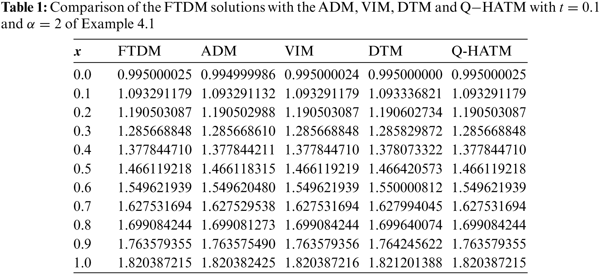
From this table, we can see that the simulated solutions from this method are very close to that obtained from other numerical techniques.

Fig. 1 explores the numerical solutions of the FTDM for diverse values of α of Example 4.1. (a) FTDM solution for α=2, (b) FTDM solution for α=1.75, (c) FTDM solution for α=1.5 and (d) FTDM solution for α=1.25.

Figure 1: FTDM solutions of different values of α in Example 4.1

Example 4.2. Consider the nonlinear FKFG equation

Dtαv(x,t)=vxx(x,t)−0.75v(x,t)+1.5v3(x,t),(27)

with the ICs

v(x,0)=−sechxandvt(x,0)=0.5sechxtanh⁡x.(28)

The exact solution of the ordinary form of Eq. (27) can be obtained by putting α=2 is v(x,t)=−sech(x+0.5t).

Solution. Applying the formable transform on both sides of Eq. (27) reveals

R[Dtαv(x,t)]=R[vxx(x,t)−0.75v(x,t)]+R[1.5v3(x,t)](29)

Using the ICs (28) and running the formable transform on Eq. (29) give

(su)αR[v(x,t)]−(su)α(−sechx)−(su)α−1(0.5sechxtanh⁡x)=R[vxx(x,t)−0.75v(x,t)+1.5v3(x,t)]

R[v(x,t)]=−sechx+us(0.5sechxtanh⁡x)+(us)αR[vxx(x,t)−0.75v(x,t)+1.5v3(x,t)].(30)

Applying the inverse formable transform to Eq. (30) implies

v(x,t)=−sechx+0.5t(sechxtanh⁡x)+R−1[(us)αR[vxx(x,t)−0.75v(x,t)+1.5v3(x,t)]].(31)

Now, decompose the nonlinear term

𝒩[v(x,t)]=v3(x,t)=∑l=0∞Al,(32)

and assume the solution of Eq. (27) have the following series representation

v(x,t)=∑l=0∞vl(x,t).(33)

Hence, substituting the series expansions (32) and (33) in Eq. (31) suggests to have

∑l=0∞vl(x,t)=−sechx+0.5t(sechxtanh⁡x)+R−1[(us)αR[∑l=0∞(vlxx(x,t)−0.75vl(x,t)+1.5Al)]].(34)

From Eq. (34), we have

v0(x,t)=−sechx+0.5t(sechxtanh⁡x).

To find v1(x,t), we find the first component of the Adomian polynomial A0,

A0=𝒩[v0(x,t)]=(v0(x,t))3=(−sechx+0.5t(sechxtanh⁡x))3

v1(x,t)=R−1[(us)αR[v0xx(x,t)−0.75v0(x,t)+1.5A0]]=R−1[(us)αR[sech3x−sechxtanh2⁡x−0.75(−sechx+0.5tsechxtanh⁡x)+1.5(−sechx+0.5tsechxtanh⁡x)3+0.5t(−4sech3xtanh⁡x+tanh⁡x(−sech3x+sechxtanh2⁡x))]]=sechx(0.75tαΓ(α+1)−0.375tα+1Γ(α+2)tanh⁡x−tαΓ(α+1)tanh2⁡x+0.5tα+1Γ(α+2)tanh3x+sech2x(−0.5tαΓ(α+1)−0.25tα+1Γ(α+2)tanh⁡x−2.25tα+2Γ(α+3)tanh2x+1.125tα+3Γ(α+4)tanh3x))

⋮

We obtain the FTDM solution by substituting v0(x,t),v1(x,t),…, in Eq. (33), as

v(x,t)≈12sechx(ttanh⁡x−2)+tαsechx8Γ(α+1)(3−cos⁡h2x)+tα+1tanh⁡xsechx2Γ(α+2)(tanh2⁡x−sech2x2−34)−9tα+2tanh2⁡xsech3x4(1Γ(α+3)−ttanh⁡x2Γ(α+4))+⋯.

Table 2 presents the simulated outcomes for various values of α and the variables x and t using the FTDM. The table shows that when α increases from 1.5 to 2 the solution converges to the exact solution and when t increases, the absolute error decreases.

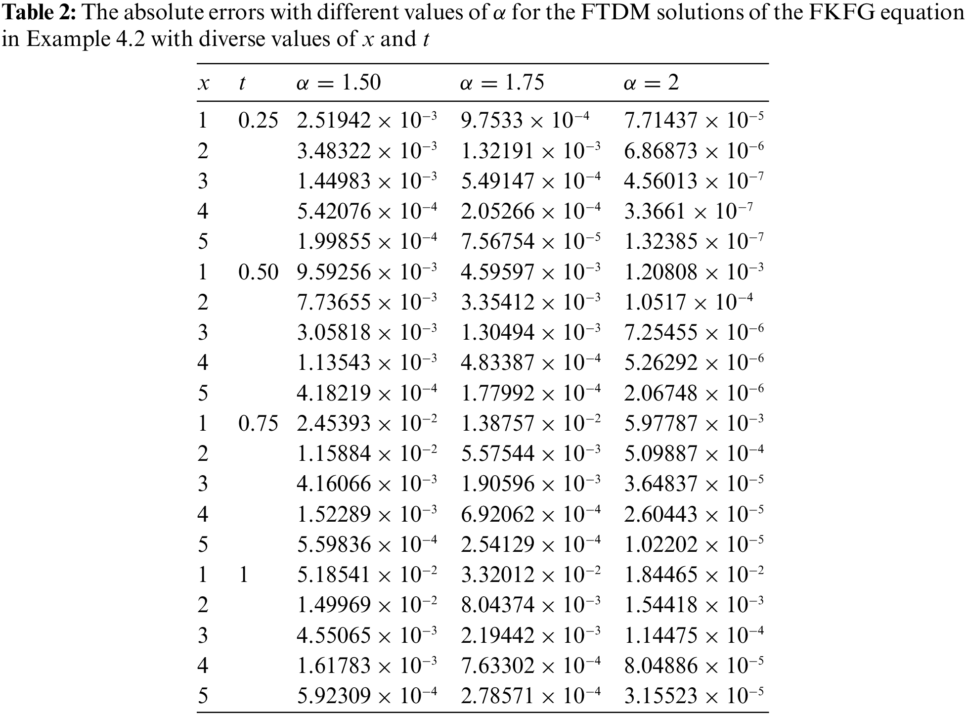
Fig. 2 explores the numerical solutions of FTDM for diverse values of α in Example 4.2. (a) FTDM solution for α=2, (b) FTDM solution for α=1.75, (c) FTDM solution for α=1.5 and (d) FTDM solution for α=1.25.

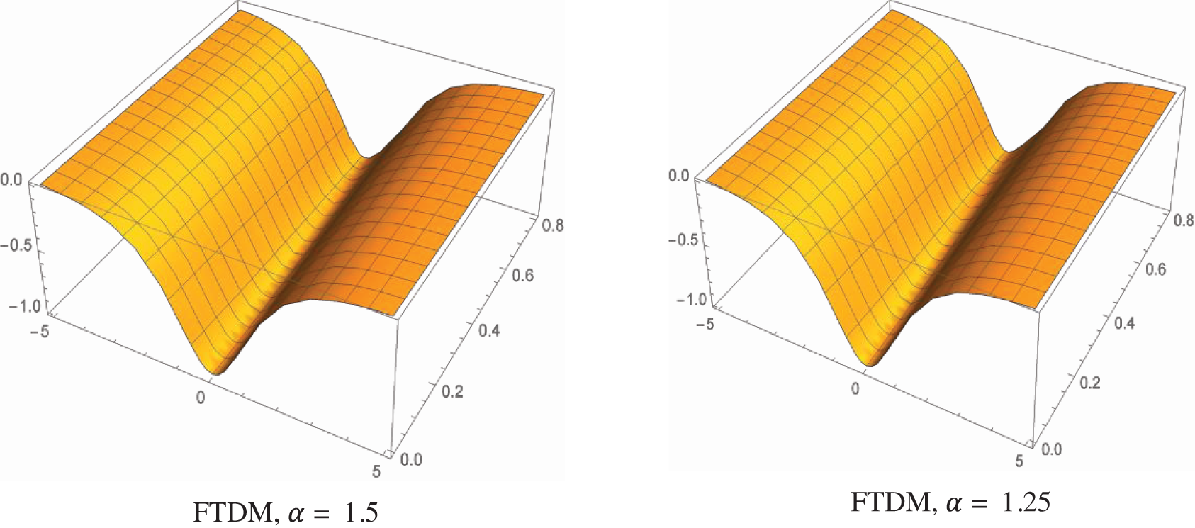
Figure 2: FTDM solutions of different values of α in Example 4.2

We can see that as α increases from α=1.25 to α=2 the graph of v(x,t) coincides with the exact solution obtained when α=2.

In Fig. 3, we present the graph of the FTDM solution obtained in Example 4.2, in 2D plots. It helps us to understand the behavior of the simulated outcomes of the model for distinct values of time.

Figure 3: Nature of FTDM solution of Example 4.2 at: (a) t=0, (b) t=1 (c) t=3 and (d) t=5 for distinct values of α

Example 4.3. Consider the nonlinear FKFG equation

Dtαv(x,t)=52vxx(x,t)−v(x,t)−32v3(x,t),

with the ICs

v(x,0)=23tan⁡(1032111x) and vt(x,0)=sec2⁡(1032111x)937.

The exact solution of the ordinary differential equation can be obtained by putting α=2 and v(x,t)=23tan⁡(1032111(t20+x)).

Solution. By employing the FTDM, we get

v0(x,t)=tsec2⁡(1032111x)937+23tan⁡(1032111x)and

v1(x,t)=sec6⁡(1032111x)2661336(637tα+1Γ(α+2)−2437tα+3Γ(α+4)+437tα+1cos⁡(2032111x)Γ(α+2)−237tα+1cos⁡(4032111x)Γ(α+2)+2226sin⁡(2032111x)(t−6tα+2Γ(α+3))437tα+1cos⁡(2032111x)Γ(α+2)+1116tsin⁡(4032111x)).

Therefore, we obtain the FTDM solution by substituting v0(x,t),v1(x,t),… in Eq. (15), to yield

v(x,t)≈tsec2⁡(1032111x)937+23tan⁡(1032111x)+sec6⁡(1032111x)2661336(637tα+1Γ(α+2)−2437tα+3Γ(α+4)+437tα+1cos⁡(2032111x)Γ(α+2)−237tα+1cos⁡(4032111x)Γ(α+2)+2226sin⁡(2032111x)(t−6tα+2Γ(α+3))437tα+1cos⁡(2032111x)Γ(α+2)+1116tsin⁡(4032111x)).

Table 3 presents the simulated outcomes for various values of α and the variables x and t using the FTDM. The table shows that when α increases from 1.5 to 2 the solution converges to the exact solution and when t increases, the absolute error decreases.

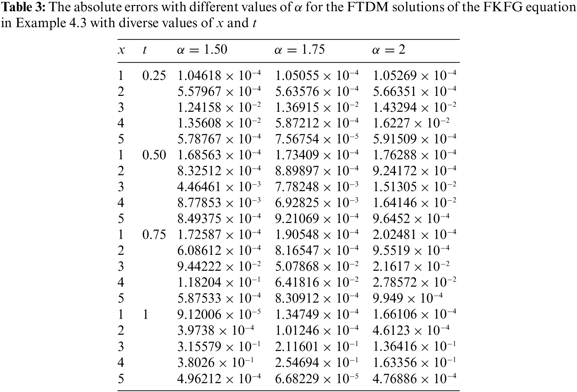
Fig. 4 explores the numerical solutions of the FTDM for diverse values of α in Example 4.3. (a) FTDM solution for α=2, (b) FTDM solution for α=1.75, (c) FTDM solution for α=1.5 and (d) FTDM solution for α=1.25. We can see that as α increases from α=1.25 to α=2 the graph of v(x,t) coincides with the exact solution obtained when α=2.

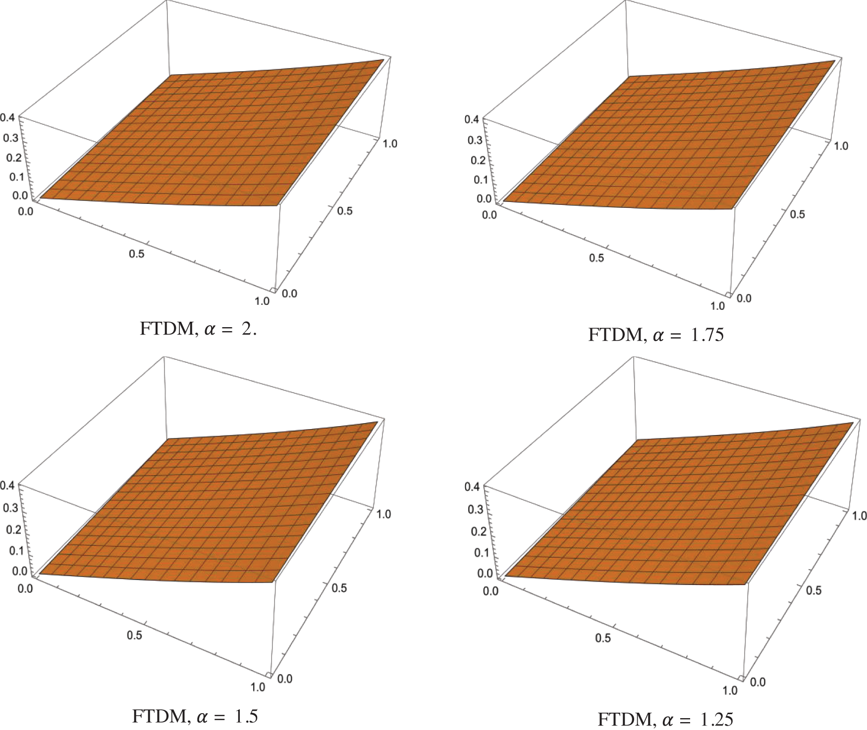
Figure 4: FTDM solutions of different values of α in Example 4.3

6  Conclusions

In this research, we have applied the formable transform to the Riemann–Liouville fractional integral operator and the Caputo fractional derivative. These new formulas are implemented to construct the approximate solutions of certain fractional differential equations in a series representation. The new technique is presented in the algorithm, and it integrates the formable integral operator with the ADM method to get a series solution of the fractional differential equations. Three interesting examples of the TFKGE are presented and solved by the new technique. Efficiency and applicability of the FTDM method, certain numerical simulations and comparisons with other methods were presented and illustrated as examples. The motivation of this research has simplified the procedure of finding the approximate solutions with fewer efforts and calculations. In the future, we intend to solve time fractional partial differential equations with initial and boundary conditions, as stated in [39,40].

Funding Statement: This research is funded by the Deanship of Research in Zarqa University, Jordan.

Availability of Data and Materials: No data were used to support this study.

Conflicts of Interest: The authors declare that they have no conflicts of interest to report regarding the present study.

References

1. Qazza, A., Hatamleh, R., Alodat, N. (2016). About the solution stability of volterra integral equation with random kernel. Far East Journal of Mathematical Sciences, 100, 671–680. https://doi.org/10.17654/MS100050671 [Google Scholar] [CrossRef]

2. Gharib, G., Saadeh, R. (2021). Reduction of the self-dual yang-mills equations to sinh-poisson equation and exact solutions. WSEAS Interactions on Mathematics, 20, 540–554. https://doi.org/10.37394/23206 [Google Scholar] [CrossRef]

3. Qazza, A., Hatamleh, R. (2018). The existence of a solution for semi-linear abstract differential equations with infinite B chains of the characteristic sheaf. International Journal of Applied Mathematics, 31, 611–620. https://doi.org/10.12732/ijam.v31i5.7 [Google Scholar] [CrossRef]

4. Saadeh, R., Al-Smadi, M., Gumah, G., Khalil, H., Khan, A. (2016). Numerical investigation for solving two-point fuzzy boundary value problems by reproducing kernel approach. Applied Mathematics & Information Sciences, 10(6), 1–13. https://doi.org/10.18576/amis/100615 [Google Scholar] [CrossRef]

5. Hilfer, R. (2000). Applications of fractional calculus in physics. River Edge, NJ: World Scientific Publishing Co., Inc. [Google Scholar]

6. Laroche, E., Knittel, D. (2005). An improved linear fractional model for robustness analysis of a winding system. Control Engineering Practice, 13, 659–666. https://doi.org/10.1016/j.conengprac.2004.05.008 [Google Scholar] [CrossRef]

7. Lai, J., Liu, F., Anh, V., Liu, Q. (2021). A space-time finite element method for solving linear riesz space fractional partial differential equations. Numer. Algorithms, 88 (1), 499–520.https://doi.org/10.1007/s11075-020-01047-9 [Google Scholar] [CrossRef]

8. Qazza, A., Hatamleh, R. (2016). Dirichlet problem in the simply connected domain, bounded by the nontrivial kind. Advances in Differential Equations and Control Processes, 17(3), 177–188. https://doi.org/10.17654/DE017030177 [Google Scholar] [CrossRef]

9. Saadeh, R. (2021). Numerical algorithm to solve a coupled system of fractional order using a novel reproducing kernel method. Alexandria Engineering Journal, 60(5), 4583–4591. https://doi.org/10.1016/j.aej.2021.03.033 [Google Scholar] [CrossRef]

10. Baleanu, D., Diethelm, K., Scalas, E., Trujillo, J. (2012). Fractional calculus: Models and numerical methods, vol. 3. Amazon.com: World Scientific Publishing Company. [Google Scholar]

11. Ahmed, S. A., Qazza, A., Saadeh, R. (2022). Exact solutions of nonlinear partial differential equations via the new double integral transform combined with iterative method. Axioms, 11(6), 247. https://doi.org/10.3390/axioms11060247 [Google Scholar] [CrossRef]

12. Altaie, S. A., Anakira, N., Jameel, A., Ababneh, O., Qazza, A. et al. (2022). Homotopy analysis method analytical scheme for developing a solution to partial differential equations in fuzzy environment. Fractal and Fractional, 6, 419. https://doi.org/10.3390/fractalfract6080419 [Google Scholar] [CrossRef]

13. Momani, S., Odibat, Z. (2007). Homotopy perturbation method for nonlinear partial differential equations of fractional order. Physics Letters A, 365(5–6), 345–350. https://doi.org/10.1016/j.physleta.2007.01.046 [Google Scholar] [CrossRef]

14. Saadeh, R., Ghazal, B. (2021). A new approach on transforms: Formable integral transform and its applications. Axioms, 10(4), 332. https://doi.org/10.3390/axioms10040332 [Google Scholar] [CrossRef]

15. Aruna, K., Kanth, V. (2013). Approximate solutions of non-linear fractional schrodinger equation via differential transform method and modified differential transform method. National Academy Science Letters, 36(2), 201–213. https://doi.org/10.1007/s40009-013-0119-1 [Google Scholar] [CrossRef]

16. Saadeh, R., Qazza, A., Burqan, A. (2020). A new integral transform: ARA transform and its properties and applications. Symmetry, 12(6), 925. https://doi.org/10.3390/sym12060925 [Google Scholar] [CrossRef]

17. Maitama, S., Zhao, W. (2021). Homotopy analysis shehu transform method for solving fuzzy differential equations of fractional and integer order derivatives. Computational and Applied Mathematics, 40, 1–30. https://doi.org/10.1007/s40314-021-01476-9 [Google Scholar] [CrossRef]

18. Qazza, A., Burqan, A., Saadeh, R. (2021). A new attractive method in solving families of fractional differential equations by a new transform. Mathematics, 9(23), 3039. https://doi.org/10.3390/math9233039 [Google Scholar] [CrossRef]

19. Freihat, A., Abu-Gdairi, R., Khalil, H., Abuteen, E., Al-Smadi, M. et al. (2016). Fitted reproducing kernel method for solving a class of third-order periodic boundary value problems. American Journal of Applied Sciences, 13(5), 501–510. https://doi.org/10.3844/ajassp.2016.501.510 [Google Scholar] [CrossRef]

20. Burqan, A., Saadeh, R., Qazza, A., Momani, S. (2023). ARA-residual power series method for solving partial fractional differential equations. Alexandria Engineering Journal, 62, 47–62. https://doi.org/10.1016/j.aej.2022.07.022 [Google Scholar] [CrossRef]

21. Shqair, M., El-Ajou, A., Nairat, M. (2019). Analytical solution for multi-energy groups of neutron diffusion equations by a residual power series method. Mathematics, 7, 633. https://doi.org/10.3390/math7070633 [Google Scholar] [CrossRef]

22. Burqan, A., Saadeh, R., Qazza, A. (2022). A novel numerical approach in solving fractional neutral pantograph equations via the ARA integral transform. Symmetry, 14(1), 50. https://doi.org/10.3390/sym14010050 [Google Scholar] [CrossRef]

23. Burqan, A., El-Ajou, A., Saadeh, R., Al-Smadi, M. (2022). A new efficient technique using Laplace transforms and smooth expansions to construct a series solution to the time-fractional Navier-Stokes equations. National Academy Science Letters, 61(2), 1069–1077. https://doi.org/10.1016/j.aej.2021.07.020 [Google Scholar] [CrossRef]

24. Whitham, B. (1974). Linear and nonlinear waves. New York: Wiley. [Google Scholar]

25. Zauderer, E. (1983). Partial differential equations of applied mathematics. New York: Wiley. [Google Scholar]

26. Perring, K., Skyrme, R. (1962). A model unified field equation. Nuclear Physics, 31, 550–555. https://doi.org/10.1016/0029-5582(62)90774-5 [Google Scholar] [CrossRef]

27. Schiff, I. (1951). Nonlinear meson theory of nuclear forces. I. Neutral scalar mesons with point-contact repulsion. Physical Review, 84(1). https://doi.org/10.1103/PhysRev.84.1 [Google Scholar] [CrossRef]

28. Adomian, G. (1986). Nonlinear stochastic operator equations. Academic Press, Kluwer Academic Publishers. [Google Scholar]

29. El-Sayed, M. (2003). The decomposition method for studying the Klein-Gordon equation. Chaos Solitons Fractals, 18(5), 1025–1030. https://doi.org/10.1016/S0960-0779(02)00647-1 [Google Scholar] [CrossRef]

30. Yusufoğlu, E. (2008). The variational iteration method for studying the Klein-Gordon equation. Applied Mathematics Letters, 21(7), 669–674. https://doi.org/10.1016/j.aml.2007.07.023 [Google Scholar] [CrossRef]

31. Kanth, V., Aruna, K. (2009). Differential transform method for solving the linear and nonlinear Klein-Gordon equation. Computation of Physics and Commutations, 180(5), 708–711. https://doi.org/10.1016/j.cpc.2008.11.012 [Google Scholar] [CrossRef]

32. Veeresha, P., Prakasha, G., Kumar, D. (2020). An efficient technique for nonlinear time-fractional Klein-Fock-Gordon equation. Applied Mathematics and Computations, 364, 124637. https://doi.org/10.1016/j.amc.2019.124637 [Google Scholar] [CrossRef]

33. Rawashdeh, M., Maitama, S. (2017). Finding exact solutions of nonlinear PDEs using the natural decomposition method. Mathematical Methods in the Applied Sciences, 40(1), 223–236. https://doi.org/10.1002/mma.3984 [Google Scholar] [CrossRef]

34. Agarwal, P., Mofarreh, F., Shah, R., Luangboon, W., Nonlaopon, K. (2021). An analytical technique, based on natural transform to solve fractional-order parabolic equations. Entropy, 23(8), 1086. https://doi.org/10.3390/e23081086 [Google Scholar] [PubMed] [CrossRef]

35. Loonker, D., Banerji, K. (2013). Solution of fractional ordinary differential equations by natural transform. International Journal of Mathematical Engineering Science, 12(2), 1–7. [Google Scholar]

36. Shehu, M., Weidong, Z. (2019). New integral transform: Shehu transform a generalization of Sumudu and Laplace transform for solving differential equations. International Journal of Analysis and Applications, 17(2), 167–190. [Google Scholar]

37. Atluri, S. N., Han, Z., Shen, S. (2003). Meshless Local Patrov-Galerkin (MLPG) approaches for weaklysingular traction & displacement boundary integral equations. Computer Modeling in Engineering & Sciences, 4(5), 507–517. https://doi.org/10.3970/cmes.2003.004.507 [Google Scholar] [CrossRef]

38. Zhao, S., Yang, Z. C., Zhou, X. G., Ling, X. Z., Mora, L. S. et al. (2014). Design, fabrication, characterization and simulation of PIP-SiC/SiC composites. Computers, Materials & Continua, 42(2), 103–124. https://doi.org/10.3970/cmc.2014.042.103 [Google Scholar] [CrossRef]

39. Kanwal, A., Phang, C., Iqbal, U. (2018). Numerical solution of fractional diffusion wave equation and fractional Klein–Gordon equation via two-dimensional Genocchi polynomials with a Ritz–Galerkin method. Computation, 6(3), 40. https://doi.org/10.3390/computation6030040 [Google Scholar] [CrossRef]

40. Phang, C., Kanwal, A., Loh, J. R. (2020). New collocation scheme for solving fractional partial differential equations. Hacettepe Journal of Mathematics and Statistics, 49(3), 1107–1125. [Google Scholar]

41. Al-Smadi, M., Djeddi, N., Momani, S., Al-Omari, S., Araci, S. (2021). An attractive numerical algorithm for solving nonlinear Caputo–Fabrizio fractional abel differential equation in a Hilbert space. Advances in Difference Equations, 2021, 271. https://doi.org/10.1186/s13662-021-03428-3 [Google Scholar] [CrossRef]

42. Alaroud, M., Tahat, N., Al-Omari, S., Suthar, D. L., Gulyaz-Ozyurt, S. (2021). An attractive approach associated with transform functions for solving certain fractional Swift-Hohenberg equation. Journal of Function Spaces, 2021, 3230272. https://doi.org/10.1155/2021/3230272 [Google Scholar] [CrossRef]

43. Alaroud, M., Ababneh, O., Tahat, N., Al-Omari, S. (2022). Analytic technique for solving temporal time-frac-424 tional gas dynamics equations with Caputo fractional derivative. AIMS Mathematics, 7, 17647–17669. https://doi.org/10.3934/math.2022972 [Google Scholar] [CrossRef]

44. Gumah, G., Naser, M. F. M., Al-Smadi, M., Al-Omari, S., Baleanu, D. (2020). Numerical solutions of hybrid 377 fuzzy differential equations in a hilbert space. Applied Numerical Mathematics, 151, 402–412. https://doi.org/10.1016/j.apnum.2020.01.008 [Google Scholar] [CrossRef]