
 Submit a Paper
 Propose a Special lssue
 Open Access
ARTICLE

Adaptive Time Slot Resource Allocation in SWIPT IoT Networks
1 Key Laboratory of Information and Communication Systems, Ministry of Information Industry, Beijing Information Science and Technology University, Beijing, 100101, China
2 Key Laboratory of Modern Measurement & Control Technology, Ministry of Education, Beijing Information Science & Technology University, Beijing, 100101, China
3 Beijing Advanced Innovation Center for Future Blockchain and Privacy Computing, Beijing, 100101, China
* Corresponding Author: Yuexia Zhang. Email:
(This article belongs to the Special Issue: Recent Advances in Backscatter and Intelligent Reflecting Surface Communications for 6G-enabled Internet of Things Networks)
Computer Modeling in Engineering & Sciences 2023, 136(3), 2787-2813. https://doi.org/10.32604/cmes.2023.027351
Received 26 October 2022; Accepted 02 December 2022; Issue published 09 March 2023
 View Full Text
 Download PDF
Abstract
The rapid advancement of Internet of Things (IoT) technology has brought convenience to people’s lives; however further development of IoT faces serious challenges, such as limited energy and shortage of network spectrum resources. To address the above challenges, this study proposes a simultaneous wireless information and power transfer IoT adaptive time slot resource allocation (SIATS) algorithm. First, an adaptive time slot consisting of periods for sensing, information transmission, and energy harvesting is designed to ensure that the minimum energy harvesting requirement is met while the maximum uplink and downlink throughputs are obtained. Second, the optimal transmit power and channel assignment of the system are obtained using the Lagrangian dual and gradient descent methods, and the optimal time slot assignment is determined for each IoT device such that the sum of the throughput of all devices is maximized. Simulation results show that the SIATS algorithm performs satisfactorily and provides an increase in the throughput by up to 14.4% compared with that of the fixed time slot allocation (FTS) algorithm. In the case of a large noise variance, the SIATS algorithm has good noise immunity, and the total throughput of the IoT devices obtained using the SIATS algorithm can be improved by up to 34.7% compared with that obtained using the FTS algorithm.Keywords
With the continuous development in communication technology, Internet of Things (IoT) has been gradually integrated into many aspects of public life (e.g., public safety, smart city, enemy reconnaissance, and many other fields) [1–6]. According to statistics, the number of Internet of Things devices (IoDs) may reach 30 billion by 2025. The widespread application of IoT enables the communication between people and things and among things at any time and place [7,8]. In addition to increasing convenience, it also promotes intelligence development in public life. Thus, the proliferation of IoT has greatly improved the quality of life, and it is of great practical significance to study IoT.
Although IoT has become an irreplaceable part of public life, the IoT system faces challenges, such as limited energy storage of the IoDs and the scarcity of spectrum resources [9]. The emergence of simultaneous wireless information and power transfer (SWIPT) technology has provided a new method of solving the problem of the limited energy of the IoDs [10]. The application of the SWIPT technology allows IoDs to harvest energy from radio frequency (RF) waves and convert it into electrical energy, which can be stored in the battery of the device, thus maximizing the usable time of the device [11,12] and reducing the additional cost of battery replacement or manual charging of the device [13]. However, there is a limit to the amount of energy that can be stored in the battery, and excessive energy harvesting puts a greater burden on the operation of the device. Less than the appropriate amount of energy disrupts the normal operation of the device, and adequate energy harvesting using SWIPT IoT enables the entire network system to continue operating. Meanwhile, the normal communication of IoDs requires the support of large amounts of the radio spectrum, and the recent shortage of spectrum resources has restricted the development of IoT [14]. Therefore, reasonable allocation of the limited spectrum resources has become the focus of research in regard to SWIPT IoT.
A number of recent studies have considered the issue of resource allocation in regard to energy harvesting in SWIPT IoT. Zhu et al. [15] determined the user maximized minimum energy harvesting subject to the secrecy rate and total transmit power constraints in the presence of channel estimation errors, ensuring the fairness of user energy harvesting. Masood et al. [16] proposed an algorithm to achieve a compromise between energy efficiency and spectral efficiency in the SWIPT system, which is based on using the Lagrange multiplier method to find the optimal solution without iterative computation. Simulation results proved that the algorithm achieved the maximum energy transmission by using the optimal power split ratio. Han et al. [17] studied fair resource allocation in terms of the maximum–minimum energy requirement for wireless power transmission in edge computing systems. They solved the nonconvex mixed-integer nonlinearity that arises when using a logarithmic nonlinear energy harvesting model by using a continuous relaxation method. Yazdani et al. [18] proposed a parametric power control method that allows each sub-user to adjust its power according to the stored energy such that the lower limit of the sum of the uplink rates is maximized. Xu et al. [19] studied the resource allocation problem with perfect channel state information under the constraints of minimum energy harvesting and quality of service. Qi et al. [20] considered channel uncertainty, receiver nonlinearity, and decoding message cancellation for imperfect continuous messages in SWIPT-based non-orthogonal multiple access (NOMA) large scale IoT in the process of designing a resource allocation method.
Researchers have also considered joint optimization and allocation of multiple resources in SWIPT IoT. Prathima et al. [21] considered a collaborative cognitive radio (CR) network with two primary and secondary users, wherein power splitting and time-switching energy harvesting techniques were used and the system throughput and energy efficiency were maximized by using a particle swarm optimization algorithm. Acosta et al. [22] jointly considered the energy harvesting of the system, data rate, and the maximum power level allowed to interfere with the users to minimize the transmit power of the auxiliary base station. They solved the external and internal optimizations using a particle swarm optimization algorithm and a semidefinite relaxation algorithm, respectively. Tuan et al. [23] investigated resource allocation with respect to maximizing the total energy harvesting and energy harvesting efficiency under linear and nonlinear energy harvesting models in a SWIPT system consisting of a multi-input single-output interference channel to jointly optimize the beam formation vector of the transmitter and the power splitting ratio of the receiver. Hu et al. [24] maximized the secrecy rate in a multi-input multi-output bidirectional relay-assisted CR NOMA network by jointly optimizing the power allocation of the users and power splitting factor under the constraints of quality of service, energy harvesting, and transmission power. Tang et al. [25] jointly optimized the transmission rate and harvested energy in a SWIPT-enabled NOMA system using power splitting to simultaneously fulfill the minimum rate and harvested energy requirements for each user. Yang et al. [26] used resource management methods based on deep reinforcement learning to jointly optimize radio allocation and control strategies of transmission power in cognitive IoT. Ramzan et al. [27] simultaneously optimized device selection, unmanned aerial vehicle (UAV) relay allocation, and power splitting ratio in an IoT system based on UAV relay communication with energy harvesting, where the optimization results showed significant advantages in the above aspects. Xiao et al. [28] maximized the energy efficiency in RF energy-driven CR networks by jointly optimizing transmission time and power control and also proposed a resource allocation scheme called the co-channel interference approximation convex strategy. These studies investigated resource allocation in regard to SWIPT IoT and obtained adequate results. However, most researchers only focused on the uplink or downlink information transmission in SWIPT IoT systems without considering that most IoDs required alternating uplink and downlink information transmissions in real-time. This problem can be addressed by jointly allocating resources for uplink and downlink information transmissions and energy harvesting in SWIPT IoT such that the results obtained can be more in line with actual situations.
The main contributions of this study are summarized as follows:
• An adaptive time slot (ATS) structure is designed that consists of a sensing time period at the beginning, time periods for several alternating uplink and downlink information transmissions, and a common time period for downlink energy harvesting and information transmission. The ATS structure allows the IoD to adaptively allocate time in a time slot to obtain the maximum uplink and downlink throughputs while satisfying the minimum energy harvesting requirements.
• A SWIPT IoT ATS resource allocation (SIATS) algorithm is proposed. The algorithm first solves the coupling problem in the optimization function by using the method of pre-setting sensing time, time allocation factor, and time slot allocation parameters and transforms the optimization function into a convex function. Second, the optimal transmit power and channel assignment of the system is obtained by using the Lagrangian dual and gradient descent methods. Finally, by comparing the throughput results with different sensing times, time allocation factors, and time slot allocation parameters, the optimal time slot allocation for each IoD is determined such that the sum of the throughputs of all IoDs in the system is maximized.
• The simulation compares the system throughput and energy harvesting when using the SIATS algorithm proposed in this paper with the fixed time slot allocation (FTS) algorithm, and analyzes in detail the effects of parameters such as sensing time, time allocation factor, and noise on the total system throughput and energy harvesting.
The SWIPT IoT network system is shown in Fig. 1, and it is composed of
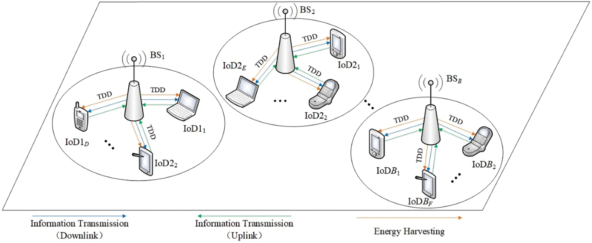
Figure 1: SWIPT IoT network system
The spectrum resources of the SWIPT IoT network system are divided into
The communication mode between the IoT base station and IoD is the time division duplex, for which an ATS structure is designed, as shown in Fig. 2.
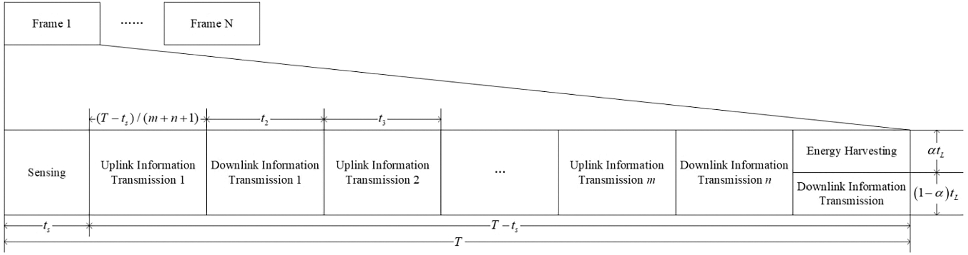
Figure 2: Adaptive time slot structure
The ATS consists of periods for sensing, uplink information transmission, downlink information transmission, and energy harvesting. The total duration of the time slot is
Furthermore, the duration of the downlink information transmission in the time period
The time period
The duration of time for the downlink information transmission is calculated as:
Finally, the duration of the complete time slot for the downlink information transmission is calculated as:
The following is an illustration of the IoT SWIPT network communication considering the IoT base station BS1 as an example; let us assume BS1 and BS2 are adjacent base stations, as shown in Fig. 1. Each IoD within the communication range of BS1 senses the state of all channels at the beginning of each time slot, and the results of the sensing are categorized into two cases.
(1) The first case: The IoD within the communication range of BS1 senses that the channel is idle. The channel is not used by the IoD within the communication range of BS1, and it is also not used by the IoD within the adjacent base station BS2. The probability of this case is assumed to be
(2) The second case: The IoD within the communication range of BS1 senses the channel is idle. The channel is not used by the IoD within the communication range of BS1, but it is used by the IoD within the neighboring base station BS2. The probability of this case is assumed to be
The two cases are discussed separately in the following section.
Based on the previous assumptions, the probability
where
where
Notably,
The IoD within the communication range of BS1 selects one or more available channels to communicate with BS1 after the sensing, and this system ensures that one channel is available for each IoD. During the communication process between BS1 and the IoD, the uplink is primarily used to transmit the information from the IoD to BS1.
The rate of transmission corresponding to IoD1i for the uplink information transmission using CHj in this case can be determined using Shannon's formula, as follows:
where the superscript
The downlink in the communication process is primarily used to send data from BS1 to the IoD within its communication range and to provide energy to the IoD when needed. Thus, the rate of transmission for the downlink information transmission between IoD1i and BS1 using CHj is computed as:
where
Based on the previous assumptions, the probability
where
In this case, the signal emitted by BS2 during the uplink information transmission with IoD2i interferes with the uplink information transmission using the co-channel within the communication range of BS1. Therefore, the rate of transmission corresponding to IoD1i during the uplink information transmission using CHj is computed as:
where the superscript
The uplink interference generated by IoD1i and BS1 using CHj for the uplink information transmission to IoD2i within the communication range of BS2 using the co-channel of CHj can be computed as:
where
The uplink throughput of IoD1i on CHj can be expressed as:
The rate of transmission for the downlink information transmission between IoD1i and BS1 performed using CHj is computed as:
where
The downlink interference generated by BS1 and IoD1i using CHj for the downlink information transmission to BS2 using the co-channel of CHj can be computed as:
The downlink throughput can be expressed as:
For energy harvesting in the downlink, a linear energy harvesting model is used in this study. Thus, the energy harvested by IoD1i using CHj can be expressed as:
where
It is assumed in this study that the IoD can simultaneously use more than one channel to communicate with the base station. Therefore, the total energy harvested by IoD1i in a time slot can be expressed as:
3 SWIPT IoT ATS Resource Allocation Algorithm
In order to achieve an optimal system, a joint optimization is performed to maximize the sum of the uplink and downlink throughputs of all IoDs within the communication range of BS1. This optimization problem can be stated as follows:
Here,
In this optimization problem, the constraint represented by Eq. (20b) indicates that the interference of the downlink information transmission within the communication range of BS1 to the downlink information transmission in BS2 using the co-channel is less than the maximum acceptable threshold for downlink interference. The constraint represented by Eq. (20c) indicates that the interference of the uplink information transmission within the communication range of BS1 to the uplink information transmission in BS2 using the co-channel is less than the maximum acceptable threshold for uplink interference. The constraint represented by Eq. (20d) indicates that the sum of the power transmitted by BS1 to the IoD within its communication range is less than the maximum transmit power of the base station. The constraint represented by Eq. (20e) indicates that the sum of the transmit power of each IoD for the uplink information transmission over the available channel is less than the maximum transmit power of the device. The constraint represented by Eq. (20f) indicates that the sum of the energy harvested by each IoD through its available channels is greater than the minimum energy harvesting requirement. The constraint represented by Eq. (20g) indicates that each channel cannot be used by more than one IoD. The constraint represented by Eq. (20h) provides the range of values for sensing time. The constraint represented by Eq. (20i) provides the range of values for the time allocation factor; The constraint in Eq. (20j) provides the range of values for the channel allocation factor. Finally, the constraints in Eqs. (20k) and (20l) ensure that neither the uplink nor downlink transmit power is less than zero.
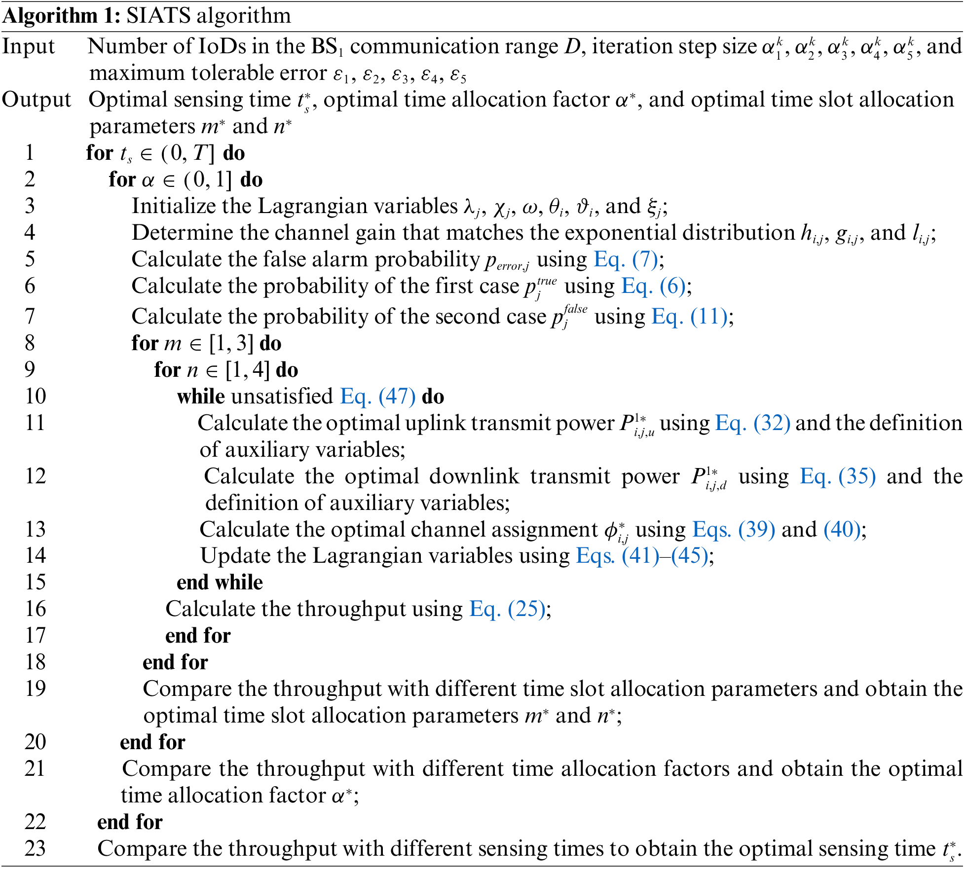
To solve the optimization problem, a SIATS algorithm is proposed in this study that can be described as follows.
The channel assignment factor
According to Eqs. (14) and (17), the optimization objective Eq. (20a) can be expressed as:
Subsequently, upon incorporating Eqs. (21)–(24) into the optimization problem in Eq. (20), it can be transformed into the formulation expressed by Eqs. (26a)–(26n):
In this optimization problem, the constraints in Eqs. (26m) and (26n) ensure that the auxiliary variables are not less than zero. The reason for adding these two constraints is that the auxiliary variables are calculated by multiplying the transmit power and the channel assignment factor, while the transmit power takes a value greater than or equal to 0 and the channel assignment factor takes a value between 0 and 1. Therefore, the auxiliary variables also need to comply with the condition that they are not less than zero. The optimization problem expressed by Eqs. (26a)–(26n) is a nonconvex problem, and a coupling exists between the sensing time
The problem, as described by Eqs. (26a)–(26n) can be transformed into a dual problem, which can be expressed as follows:
where
According to the principle of the Karush–Kuhn–Tucker (KKT) condition, the partial derivative of the Lagrangian function with respect to
where
The partial derivative of Lagrangian function with respect to
For
According to the principle of the KKT condition, the partial derivative of the Lagrangian function with respect to
Furthermore,
The partial derivative of L with respect to
For
According to the principle of the KKT condition, the partial derivative of the Lagrangian function with respect to
The partial derivative of the L with respect to
Let
In order to maximize the system throughput, different channel assignments are compared, and the result that maximizes
After determining the optimal
where
The five partial derivatives in Eq. (41) can be computed as:
The new Lagrangian variables obtained by Eqs. (41)–(46) are compared with the old values, and the iteration ends when it satisfies Eq. (47). Otherwise, the gradient descent step is repeated. Notably,
where
Based on the above mentioned process, the overall flow of the SIATS algorithm is described as follows:
:
The complexity of the SIATS algorithm proposed in this paper is jointly determined by the cyclic iterations of the four pre-set parameters and the Lagrangian dual problem iterations. The complexity of the four pre-set parameters sensing time ts, time allocation factor
4 Simulation Results and Analysis
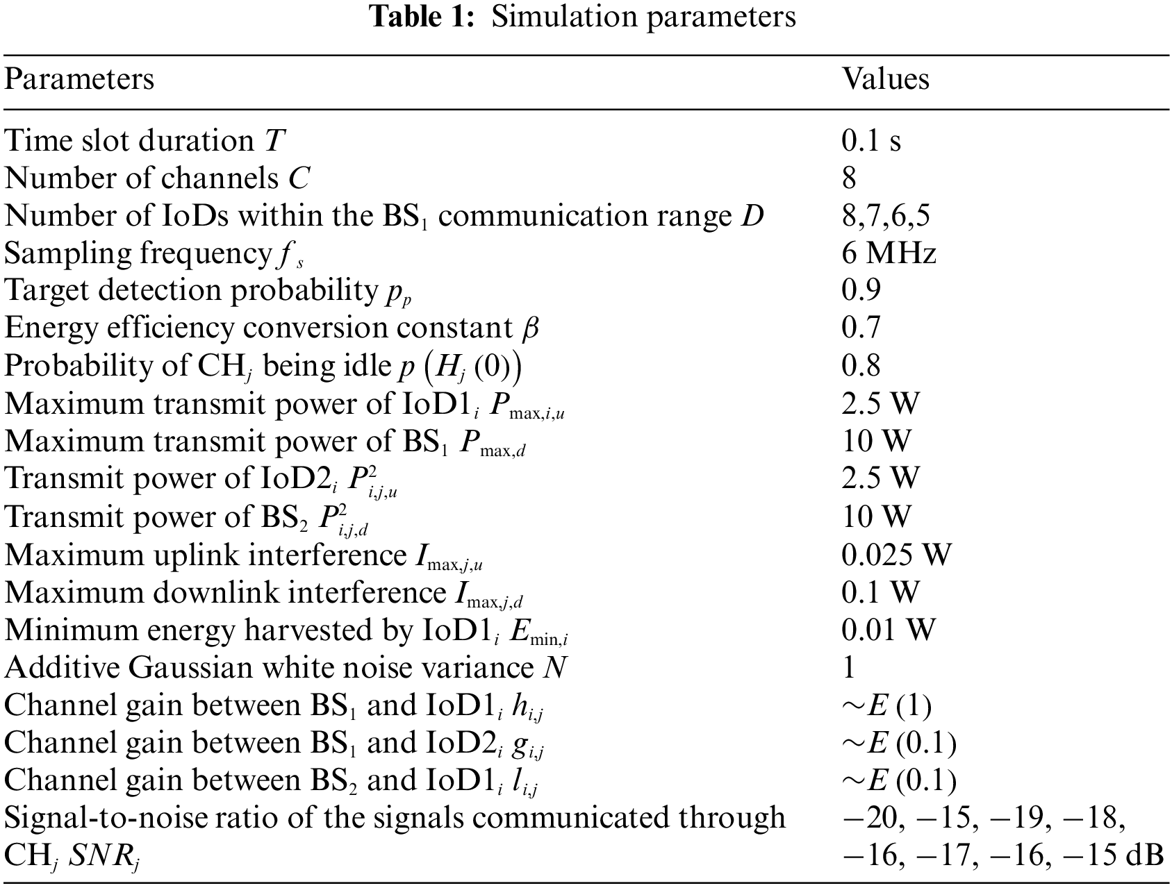
In this section, the effectiveness of the SIATS algorithm is verified using simulations. During the simulation, it is assumed that all channels in the system conform to the Rayleigh fading channel model [29–31] and that the channel gains follow an exponential distribution. It is also assumed that a total of eight channels are available for the IoDs in the entire system. Some of the parameter settings referred to in this section have been reported previously [32–35], and the specific parameter values are listed in Table 1.
The simulation is performed for four cases in which the number of IoDs within the communication range of BS1 communication range are 8, 7, 6, and 5. For the convenience of subsequent calculations, the channel bandwidth is fixed at 1 Hz, therefore, the unit of throughput is expressed as bit/s/Hz [36].
Moreover, the throughput and energy harvesting results obtained during the simulation using the proposed SIATS and FTS algorithms are compared in this study.
The time slot structure in the FTS algorithm is shown in Fig. 3, and it consists of periods for sensing, uplink information transmission, downlink information transmission, and energy harvesting. The total duration of the time slot is
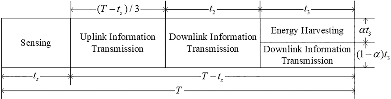
Figure 3: Fixed time slot structure
During the simulation, several scenarios may occur when performing the channel assignments. Fig. 4 shows one of the possible scenarios when the number of IoDs within the communication range of BS1 is 8, 7, 6, and 5. The horizontal coordinates in Fig. 4 represent the channel number, and the vertical coordinates represent the IoD number. The shaded cells in the figure indicate that the corresponding channel is assigned to the IoD, while the blank cells indicate that the corresponding channel is not available for use by the IoD. For example, in Fig. 4a, the first row indicates that CH1 is used by IoD16 and the third row indicates that CH3 is used by IoD12.
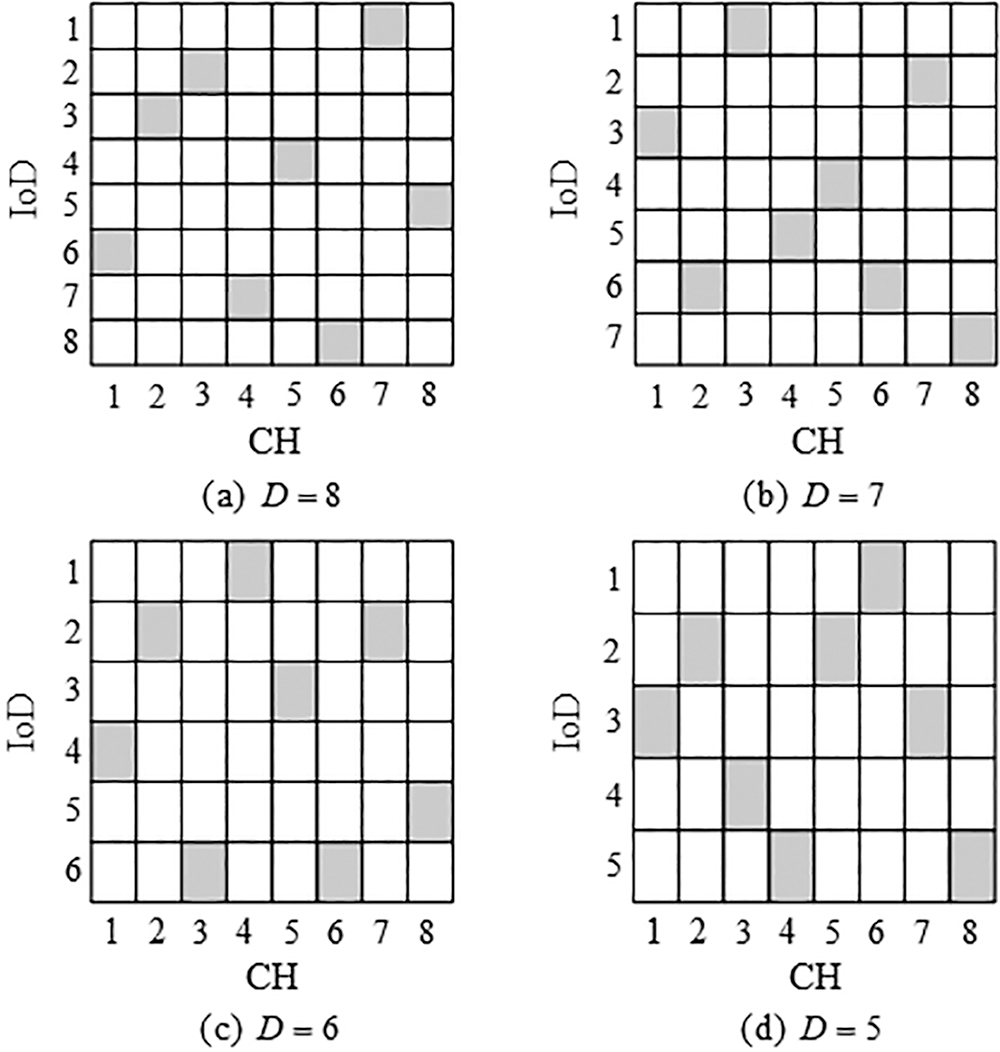
Figure 4: Example of channel assignment. (a) Number of IoDs D = 8; (b) Number of IoDs D = 7; (c) Number of IoDs D = 6; and (d) Number of IoDs D = 5
Fig. 5 presents a comparison of the variation in the system throughput with sensing time obtained using the proposed SIATS algorithm with that obtained using FTS algorithm. The horizontal coordinate represents the sensing time, and the vertical coordinate represents the total throughput of all IoDs within the communication range of BS1. The figure provides a comparison of the total throughput of the proposed SIATS and FTS algorithms for D = 8, 7, 6, and 5. The total throughput obtained by using both algorithms with different numbers of IoDs shows a trend of increasing and then decreasing with the increase in the sensing time. The reason for this is that the increase in the sensing time gradually decreases the probability of false alarm, thus increasing the throughput of the system. Additionally, the increase in the sensing time leads to a decrease in the information transmission time that reduces the throughput, thus corresponding to the decreasing trend of the variation. Comparing the curves for the same algorithm for different numbers of IoDs demonstrates that the total throughput increases as the number of IoDs increases, provided that the number of IoDs does not exceed the number of channels. Comparing the curves for different algorithms for the same number of IoDs demonstrates that the throughputs obtained using the SIATS algorithm can be increased by 14.4%, 13.4%, 12.2%, and 10.8% compared with that obtained using the FTS algorithm for D = 8, 7, 6, and 5, respectively. The throughput obtained by using the proposed SIATS algorithm is greater than that obtained by using the FTS algorithm, and the proposed algorithm exhibits better performance in terms of the throughput.
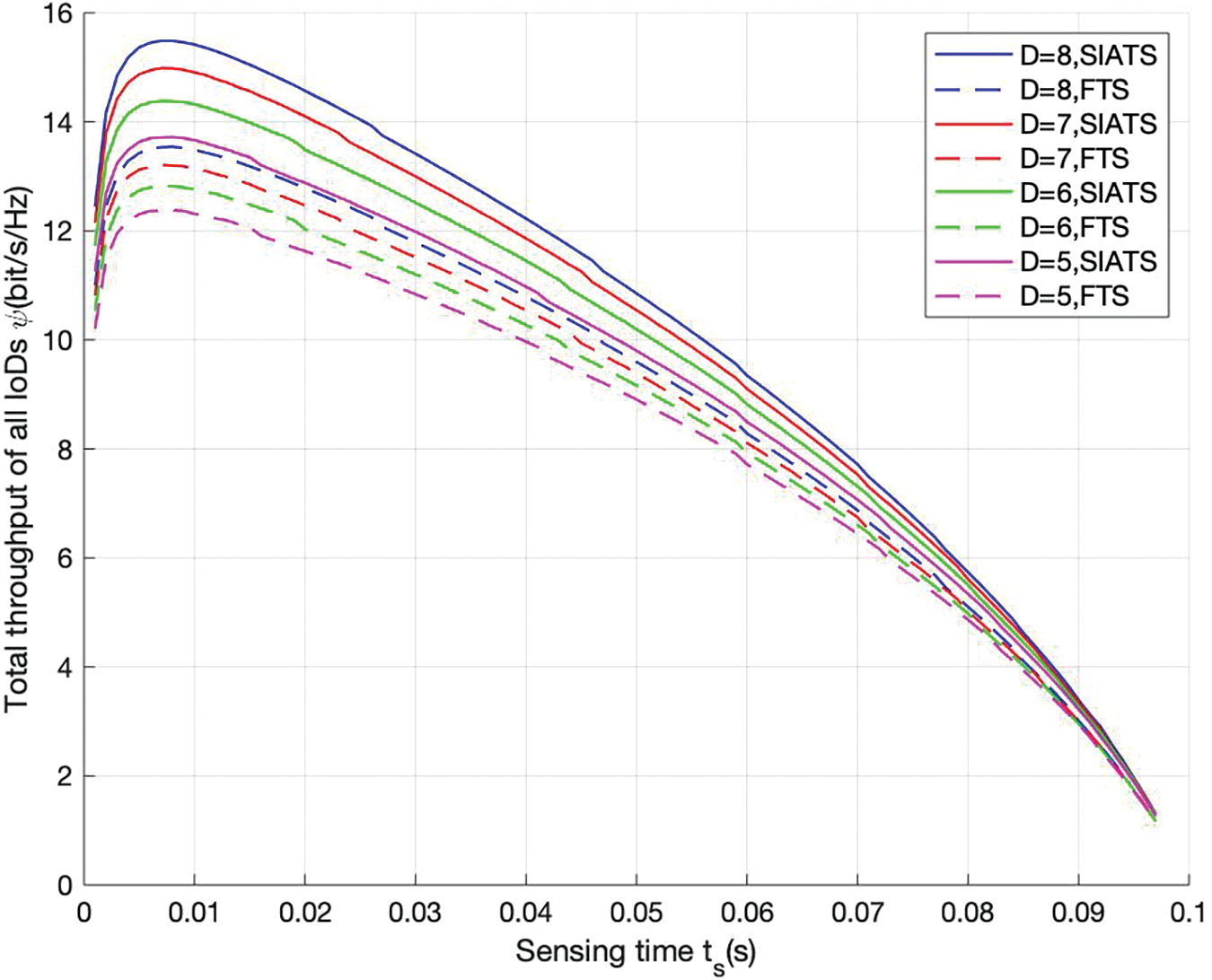
Figure 5: Variation in total throughput of all IoDs within the communication range of BS1 communication with sensing time
Fig. 6 presents a comparison of the variation in the system throughput with the time allocation factor obtained using the proposed SIATS and FTS algorithms when the sensing time is fixed at ts = 0.008 s. The horizontal coordinate represents the value of the time allocation factor
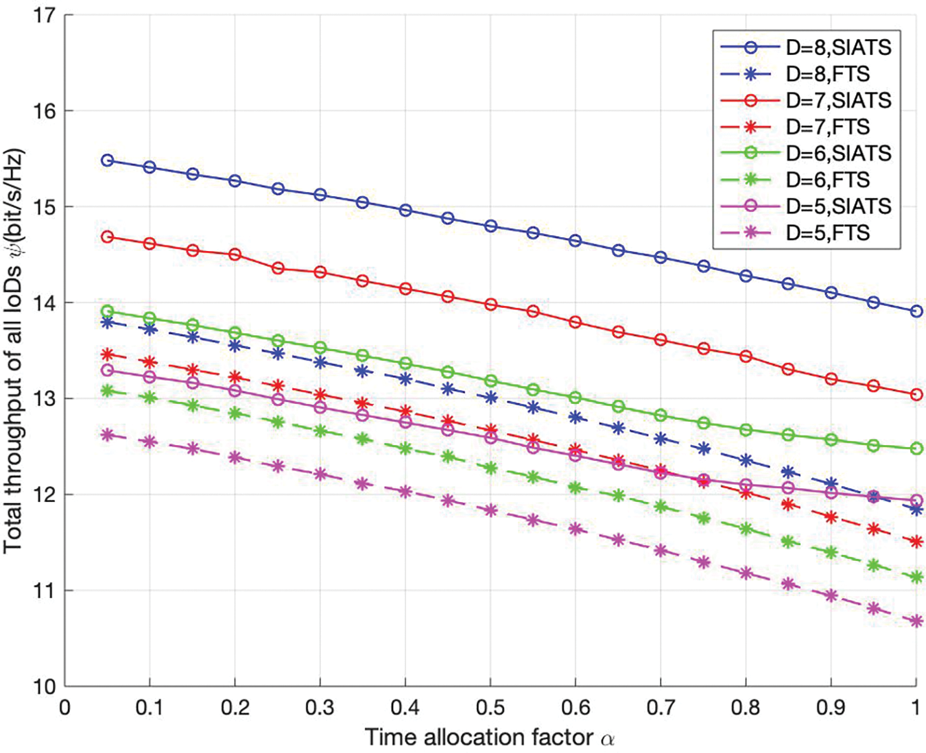
Figure 6: Variation in the total throughput of all IoDs within the communication range of BS1 with the time allocation factor
Fig. 7 presents the comparison of the energy harvested by each IoD in the proposed SIATS with that in the FTS algorithm when the time allocation factor is fixed at
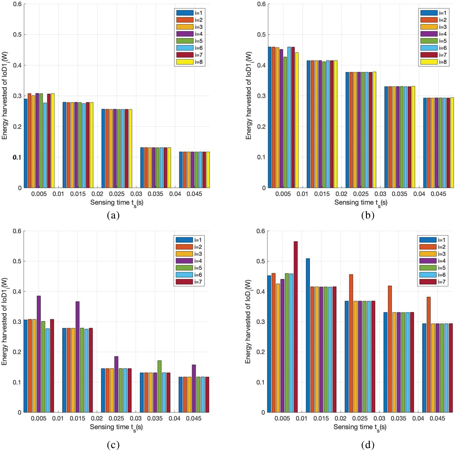
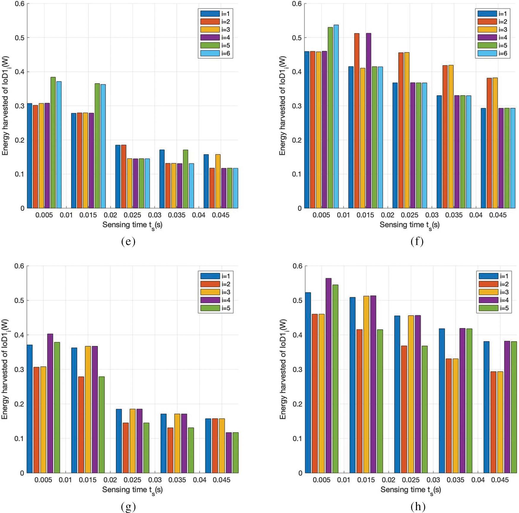
Figure 7: Energy harvesting for IoDi. (a) D = 8, SIATS algorithm; (b) D = 8, FTS algorithm; (c) D = 7, SIATS algorithm; (d) D = 7, FTS algorithm; (e) D = 6, SIATS algorithm; (f) D = 6, FTS algorithm; (g) D = 5, SIATS algorithm; and (h) D = 5, FTS algorithm
Fig. 8 presents a comparison for the total throughput of all IoDs, the throughput of a single IoD with maximum throughput, and the throughput of a single IoD with minimum throughput for different noise variances obtained by using the proposed SIATS algorithm and FTS algorithms. In the figure, the horizontal coordinates represent the Gaussian white noise variance, and the vertical coordinates represents the throughput. The figure compares the throughput of the proposed SIATS algorithm with that of the FTS algorithm for D = 8 and 5. As can be seen from the figures, the total throughput of all IoDs, the throughput of a single IoD with maximum throughput, and the throughput of a single IoD with minimum throughput obtained using the SIATS and FTS algorithms for different numbers of IoDs decrease with increasing noise variance. This is because increasing the noise variance decreases the information transfer rate and thus reduces the throughput. Comparing the results of the two algorithms, it can be concluded that the total throughput of all IoDs, the throughput of a single IoD with maximum throughput, and the throughput of a single IoD with minimum throughput obtained using the SIATS algorithm are 34.7%, 28.0%, and 33.4% higher than that obtained using the FTS algorithm, respectively, for D = 8 and a noise variance of 2. The total throughput of all IoDs, the throughput of a single IoD with maximum throughput, and the throughput of a single IoD with minimum throughput obtained using the SIATS algorithm are 34.0%, 30.9%, and 32.1% higher than that obtained using the FTS algorithm, respectively, for D = 5 and a noise variance of 2. The total throughput of all IoDs and the throughputs of a single IoD with maximum throughput, and a single IoD with minimum throughput obtained using the proposed SIATS algorithm are higher compared with that obtained using the FTS algorithm when the noise variance is large. Therefore, it can be concluded that the SIATS algorithm has good noise immunity.
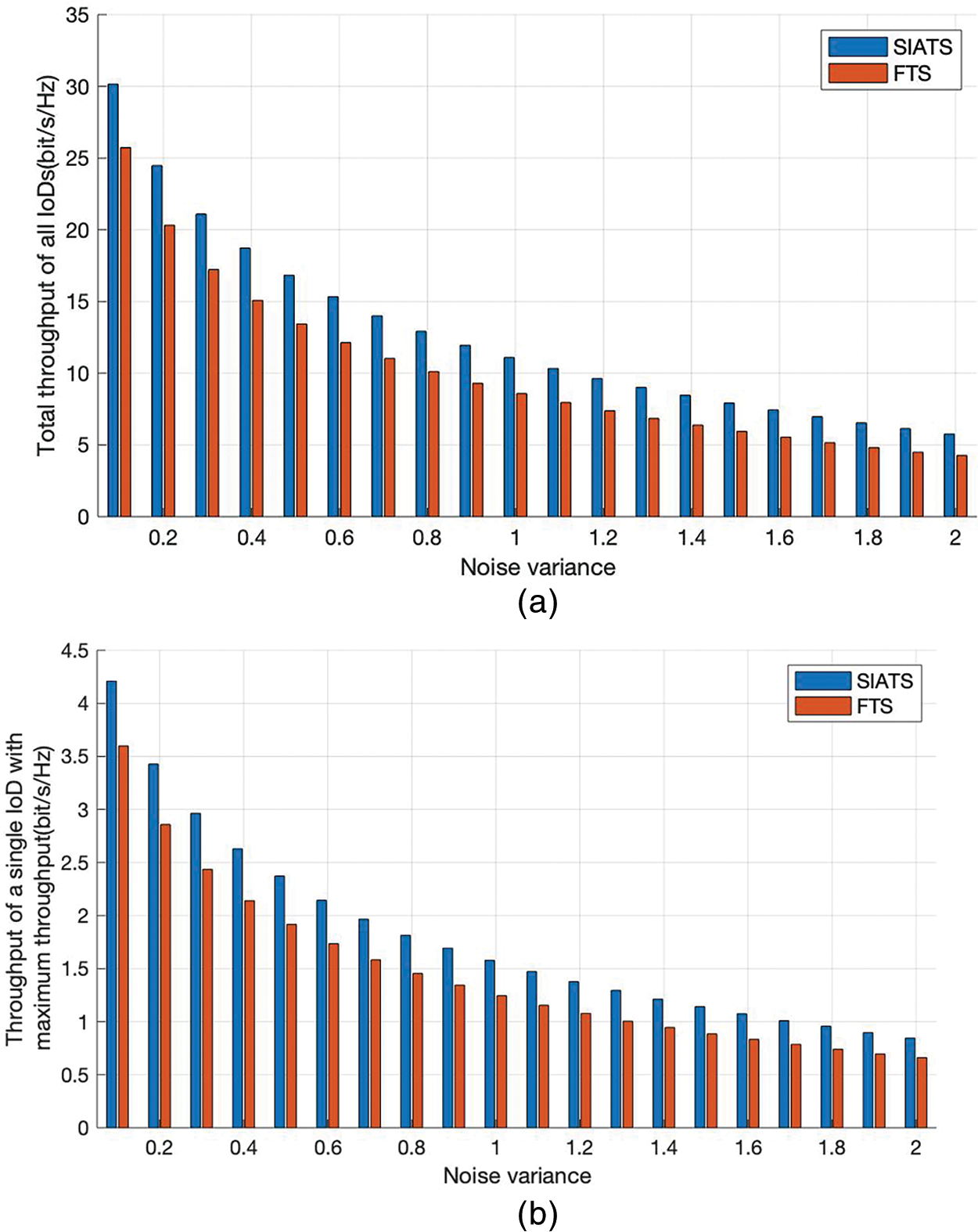
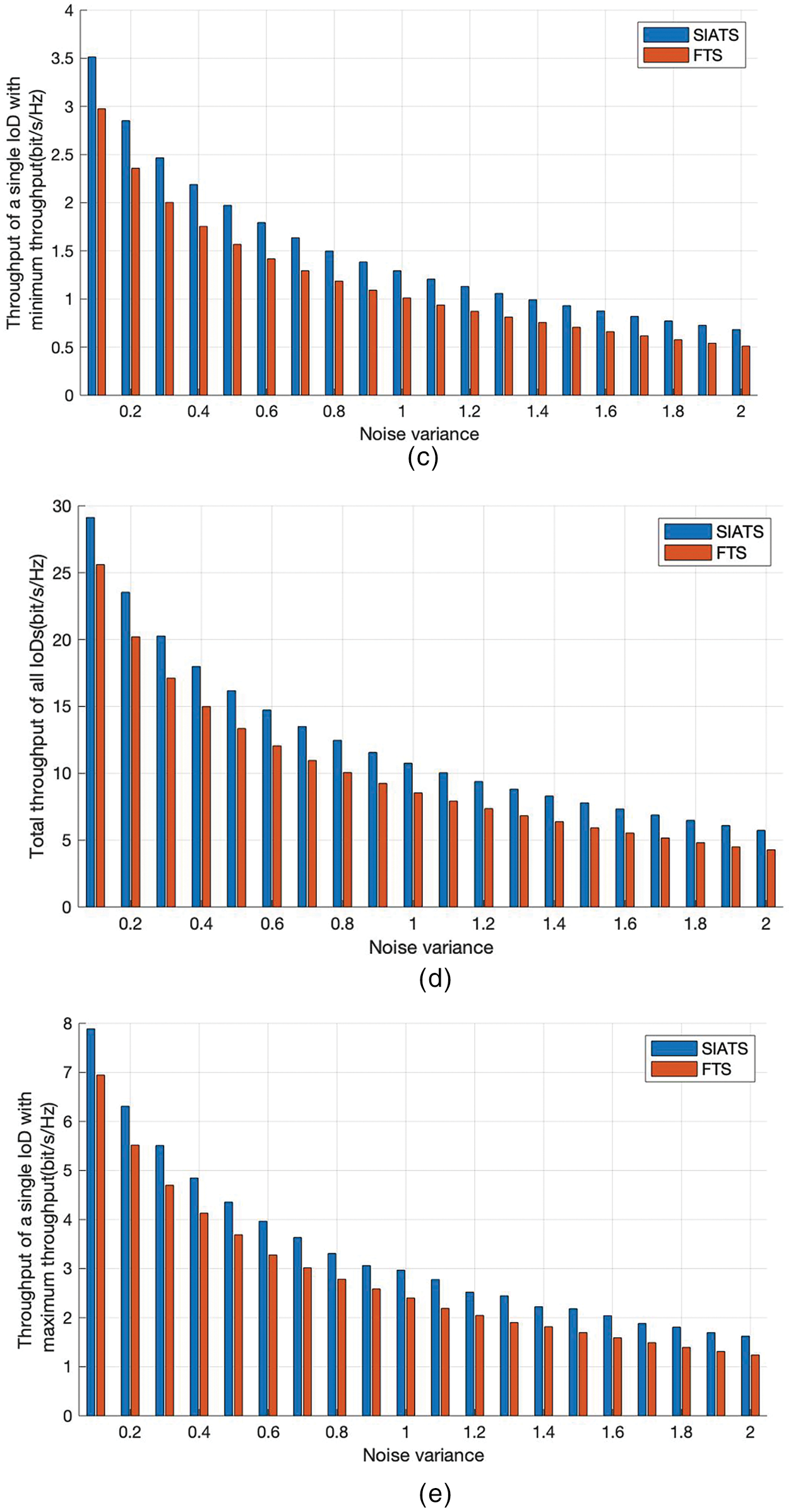

Figure 8: IoD throughput at different noise variances. (a) D = 8, total throughput of all IoDs; (b) D = 8, throughput of a single IoD with maximum throughput; (c) D = 8, throughput of a single IoD with minimum throughput; (d) D = 5, total throughput of all IoDs; (e) D = 5, throughput of a single IoD with maximum throughput; and (f) D = 5, throughput of a single IoD with minimum throughput
In this study, the SIATS algorithm is proposed to solve the coupling problem in the optimization of resource allocation by using the method of pre-setting the sensing time, time allocation factor, and time slot allocation parameters. Additionally, the optimal transmit power and channel assignment of the system are obtained by using the Lagrangian dual and gradient descent methods. Finally, the optimal time slot parameters of the SIATS algorithm are determined by comparing the throughput results for different values of the sensing time, time allocation factor, and time slot allocation parameters. Simulation results show that the proposed SIATS algorithm performs better, with a maximum throughput improvement of 14.4%, than the FTS algorithm. Meanwhile, by using the SIATS algorithm, the IoD can harvest less energy while satisfying its energy harvesting requirements, thus devoting more time to information transmission. In the case of a large noise variance, the SIATS algorithm displays good noise immunity, and the total throughput of all IoDs obtained using the SIATS algorithm can be improved by up to 34.7% compared with that obtained using the FTS algorithm. Furthermore, throughputs of the best-performing and worst-performing IoDs both improve upon using the proposed SIATS algorithm.
Funding Statement: The work was supported in part by Sub Project of National Key Research and Development Plan in 2020. No. 2020YFC1511704, Beijing Information Science & Technology University. Nos. 2020KYNH212, 2021CGZH302, Beijing Science and Technology Project (Grant No. Z211100004421009), and in part by the National Natural Science Foundation of China (Grant No. 61971048).
Conflicts of Interest: The authors declare that they have no conflicts of interest to report regarding the present study.
References
1. An, H., Park, H. (2022). Energy-balancing resource allocation for wireless cooperative IoT networks with SWIPT. IEEE Internet of Things Journal, 9(14), 12258–12271. https://doi.org/10.1109/JIOT.2021.3135282 [Google Scholar] [CrossRef]
2. Sun, L., Wang, Y., Qu, Z., Xiong, N. N. (2022). BeatClass: A sustainable ECG classification system in IoT-based eHealth. IEEE Internet of Things Journal, 9(10), 7178–7195. https://doi.org/10.1109/JIOT.2021.3108792 [Google Scholar] [CrossRef]
3. Pavani, B., Devi, L. N., Subbareddy, K. V. (2022). Energy enhancement and efficient route selection mechanism using H-SWIPT for multi-hop IoT networks. Intelligent and Converged Networks, 3(2), 173–189. https://doi.org/10.23919/ICN.2022.0013 [Google Scholar] [CrossRef]
4. Shukla, A. K., Sharanya, J., Yadav, K., Upadhyay, P. K. (2022). Exploiting SWIPT-enabled IoT-based cognitive nonorthogonal multiple access with coordinated direct and relay transmission. IEEE Sensors Journal, 22(19), 18988–18999. https://doi.org/10.1109/JSEN.2022.3198627 [Google Scholar] [CrossRef]
5. Luo, Y., Pu, L. (2021). Practical issues of RF energy harvest and data transmission in renewable radio energy powered IoT. IEEE Transactions on Sustainable Computing, 6(4), 667–678. https://doi.org/10.1109/TSUSC.2020.3000085 [Google Scholar] [CrossRef]
6. Sandhu, M. M., Khalifa, S., Jurdak, R., Portmann, M. (2021). Task scheduling for energy-harvesting-based IoT: A survey and critical analysis. IEEE Internet of Things Journal, 8(18), 13825–13848. https://doi.org/10.1109/JIOT.2021.3086186 [Google Scholar] [CrossRef]
7. Lombardi, M., Pascale, F., Santaniello, D. (2021). Internet of Things: A general overview between architectures, protocols and applications. Information, 12(2), 87. https://doi.org/10.3390/info12020087 [Google Scholar] [CrossRef]
8. Li, X., Xie, Z., Chu, Z., Menon, V. G., Mumtaz, S. et al. (2022). Exploiting benefits of IRS in wireless powered NOMA networks. IEEE Transactions on Green Communications and Networking, 6(1), 175–186. https://doi.org/10.1109/TGCN.2022.3144744 [Google Scholar] [CrossRef]
9. Sun, W., Song, Q., Zhao, J., Guo, L., Jamalipour, A. (2022). Adaptive resource allocation in SWIPT-enabled cognitive IoT networks. IEEE Internet of Things Journal, 9(1), 535–545. https://doi.org/10.1109/JIOT.2021.3084472 [Google Scholar] [CrossRef]
10. Krikidis, I., Timotheou, S., Nikolaou, S., Zheng, G., Ng, D. W. K. et al. (2014). Simultaneous wireless information and power transfer in modern communication systems. IEEE Communications Magazine, 52(11), 104–110. https://doi.org/10.1109/MCOM.2014.6957150 [Google Scholar] [CrossRef]
11. Kwon, G., Park, H., Win, M. Z. (2021). Joint beamforming and power splitting for wideband millimeter wave SWIPT systems. IEEE Journal of Selected Topics in Signal Processing, 15(5), 1211–1227. https://doi.org/10.1109/JSTSP.2021.3089026 [Google Scholar] [CrossRef]
12. Liu, Y., Han, F., Zhao, S. (2022). Flexible and reliable multiuser SWIPT IoT network enhanced by UAV-mounted intelligent reflecting surface. IEEE Transactions on Reliability, 71(2), 1092–1103. https://doi.org/10.1109/TR.2022.3161336 [Google Scholar] [CrossRef]
13. Wang, Y., Yang, K., Wan, W., Zhang, Y., Liu, Q. (2021). Energy-efficient data and energy integrated management strategy for IoT devices based on RF energy harvesting. IEEE Internet of Things Journal, 8(17), 13640–14651. https://doi.org/10.1109/JIOT.2021.3068040 [Google Scholar] [CrossRef]
14. Ali, A., Feng, L., Bashir, A. K., EI-Sappagh, S., Ahmed, S. H. (2020). Quality of service provisioning for heterogeneous services in cognitive radio-enabled Internet of Things. IEEE Transactions on Network Science and Engineering, 7(1), 328–342. https://doi.org/10.1109/TNSE.2018.2877646 [Google Scholar] [CrossRef]
15. Zhu, Z., Wang, N., Hao, W., Wang, Z., Lee, I. (2021). Robust beamforming designs in secure MIMO SWIPT IoT networks with a nonlinear channel model. IEEE Internet of Things Journal, 8(3), 1702–1715. https://doi.org/10.1109/JIOT.2020.3014933 [Google Scholar] [CrossRef]
16. Masood, Z., Park, H., Jang, H. S., Yoo, S., Jung, S. P. et al. (2021). Optimal power allocation for maximizing energy efficiency in DAS-based IoT network. IEEE Systems Journal, 15(2), 2342–2348. https://doi.org/10.1109/JSYST.2020.3013693 [Google Scholar] [CrossRef]
17. Han, J., Lee, G. H., Park, S., Choi, J. K. (2022). Joint subcarrier and transmission power allocation in OFDMA-based WPT system for mobile-edge computing in IoT environment. IEEE Internet of Things Journal, 9(16), 15039–15052. https://doi.org/10.1109/JIOT.2021.3103768 [Google Scholar] [CrossRef]
18. Yazdani, H., Vosoughi, A. (2021). Steady-state rate-optimal power adaptation in energy harvesting opportunistic cognitive radios with spectrum sensing and channel estimation errors. IEEE Transactions on Green Communications and Networking, 5(4), 2104–2120. https://doi.org/10.1109/TGCN.2021.3087456 [Google Scholar] [CrossRef]
19. Xu, Y., Sun, H., Ye, Y. (2021). Distributed resource allocation for SWIPT-based cognitive Ad-hoc networks. IEEE Transactions on Cognitive Communications and Networking, 7(4), 1320–1332. https://doi.org/10.1109/TCCN.2021.3068396 [Google Scholar] [CrossRef]
20. Qi, Q., Chen, X., Ng, D. W. K. (2020). Robust beamforming for NOMA-based cellular massive IoT with SWIPT. IEEE Transactions on Signal Processing, 68, 211–224. https://doi.org/10.1109/TSP.2019.2959246 [Google Scholar] [CrossRef]
21. Prathima, A., Gurjar, D. S., Nguyen, H. H., Bhardwaj, A. (2020). Performance analysis and optimization of bidirectional overlay cognitive radio networks with hybrid-SWIPT. IEEE Transactions on Vehicular Technology, 69(11), 13467–13481. https://doi.org/10.1109/TVT.2020.3029067 [Google Scholar] [CrossRef]
22. Acosta, M. R. C., Moreta, C. E. G., Koo, I. (2021). Joint power allocation and power splitting for MISO-RSMA cognitive radio systems with SWIPT and information decoder users. IEEE Systems Journal, 15(4), 5289–5300. https://doi.org/10.1109/JSYST.2020.3032725 [Google Scholar] [CrossRef]
23. Tuan, P. V., Koo, I. (2020). Optimizing efficient energy transmission on a SWIPT interference channel under linear/nonlinear EH models. IEEE Systems Journal, 14(1), 457–468. https://doi.org/10.1109/JSYST.2019.2924265 [Google Scholar] [CrossRef]
24. Hu, C., Li, Q., Zhang, Q., Qin, J. (2022). Security optimization for an AF MIMO two-way relay-assisted cognitive radio nonorthogonal multiple access networks with SWIPT. IEEE Transactions on Information Forensics and Security, 17, 1481–1496. https://doi.org/10.1109/TIFS.2022.3163842 [Google Scholar] [CrossRef]
25. Tang, J., Yu, Y., Liu, M., So, D. K. C., Zhang, X. et al. (2020). Joint power allocation and splitting control for SWIPT-enabled NOMA systems. IEEE Transactions on Wireless Communications, 19(1), 120–133. https://doi.org/10.1109/TWC.2019.2942303 [Google Scholar] [CrossRef]
26. Yang, H., Zhong, W., Chen, C., Alphones, A., Du, P. (2020). Deep-reinforcement-learning-based energy-efficient resource management for social and cognitive Internet of Things. IEEE Internet of Things Journal, 7(6), 5677–5689. https://doi.org/10.1109/JIOT.2020.2980586 [Google Scholar] [CrossRef]
27. Ramzan, M. R., Naeem, M., Altaf, M., Ejaz, W. (2022). Multicriterion resource management in energy-harvested cooperative UAV-enabled IoT networks. IEEE Internet of Things Journal, 9(4), 2944–2959. https://doi.org/10.1109/JIOT.2021.3094810 [Google Scholar] [CrossRef]
28. Xiao, H., Jiang, H., Shi, F., Luo, Y., Deng, L. et al. (2021). Energy-efficient resource allocation in radio-frequency-powered cognitive radio network for connected vehicles. IEEE Transactions on Intelligent Transportation Systems, 22(8), 5426–5436. https://doi.org/10.1109/TITS.2020.3026746 [Google Scholar] [CrossRef]
29. Shahini, A., Kiani, A., Ansari, N. (2019). Energy efficient resource allocation in EH-enabled CR networks for IoT. IEEE Internet of Things Journal, 6(2), 3186–3193. https://doi.org/10.1109/JIOT.2018.2880190 [Google Scholar] [CrossRef]
30. Vu, T., Nguyen, T., Kim, S. (2022). Cooperative NOMA-enabled SWIPT IoT networks with imperfect SIC: Performance analysis and deep learning evaluation. IEEE Internet of Things Journal, 9(3), 2253–2266. https://doi.org/10.1109/JIOT.2021.3091208 [Google Scholar] [CrossRef]
31. Zhang, Y., He, W., Li, X., Peng, H., Rabie, K. et al. (2022). Covert communication in downlink NOMA systems with channel uncertainty. IEEE Sensors Journal, 22(19), 19101–19112. https://doi.org/10.1109/JSEN.2022.3201319 [Google Scholar] [CrossRef]
32. Stotas, S., Nallanathan, A. (2011). Optimal sensing time and power allocation in multiband cognitive radio networks. IEEE Transactions on Communications, 59(1), 226–235. https://doi.org/10.1109/TCOMM.2010.110310.090473 [Google Scholar] [CrossRef]
33. Zhou, F., Li, Z., Cheng, J., Li, Q., Si, J. (2017). Robust AN-aided beamforming and power splitting design for secure MISO cognitive radio with SWIPT. IEEE Transactions on Wireless Communications, 16(4), 2450–2464. https://doi.org/10.1109/TWC.2017.2665465 [Google Scholar] [CrossRef]
34. Yang, H., Ye, Y., Chu, X., Dong, M. (2020). Resource and power allocation in SWIPT-enabled device-to-device communications based on a nonlinear energy harvesting model. IEEE Internet of Things Journal, 7(11), 10813–10825. https://doi.org/10.1109/JIOT.2020.2988512 [Google Scholar] [CrossRef]
35. Ma, R., Wu, H., Ou, J., Yang, S., Gao, Y. (2020). Power splitting-based SWIPT systems with full-duplex jamming. IEEE Transactions on Vehicular Technology, 69(9), 9822–9836. https://doi.org/10.1109/TVT.2020.3002976 [Google Scholar] [CrossRef]
36. Li, G., Liu, H., Huang, G., Li, X., Raj, B. et al. (2021). Effective capacity analysis of reconfigurable intelligent surfaces aided NOMA network. EURASIP Journal on Wireless Communications and Networking, 198(1), 1–16. https://doi.org/10.1186/s13638-021-02070-7 [Google Scholar] [CrossRef]
Cite This Article
 Copyright © 2023 The Author(s). Published by Tech Science Press.
This work is licensed under a Creative Commons Attribution 4.0 International License , which permits unrestricted use, distribution, and reproduction in any medium, provided the original work is properly cited.
 Downloads
 Citation Tools