Ensemble Model for Spindle Thermal Displacement Prediction of Machine Tools

1  Introduction

Since the start of the Industrial Revolution, the machine tool has played an important role and is called the mother of all machines. Literature [1] indicated “Often, the condition of a machine tool is detected indirectly in the reduced quality of manufactured parts upon visual inspection.” However, intelligent manufacturing has become a new trend with the arrival of Industry 4.0 and the rapid advancement of machine tool technologies. The demand for higher machining precision increases as the development of smart machine tool [2]. Heat induced spindle deformation, among many other factors [3], affects machining precision [4,5]. Research has shown that 40% to 70% of errors result from the heat generated by rotating spindle when the machine tool is in operation [6]. The heat of an operating machine tool comes largely from both internal and external sources [7], which were the main causes for spindle deformation and consequent machining errors [8]. Three methods [9] were used to reduce spindle thermal deformation and machining errors. The first method relies on thermal affinity design and lathes cooling technique to prevent thermal deformation. Or graphite-carbon composites were used as lathe structure material because it has the advantage of low expansion and high thermal conductivity. However, the high cost and difficulty of maintenance were the downsides. The second method implements thermal compensation by measuring thermal displacement with a laser or touch probe. The deformation was measured with the laser emitter installed on the machine and controlled by a controller. The drawback is that the laser beam cannot be used for measurement during machining operation. The third method is to model the relationships between temperature and tooltip displacement [10,11]. Since machine tool is a dynamic system and the model fails after a long operation, the capabilities of fast modeling that requires only a small amount of data and fast real-time model modification were necessary.

Many research papers about thermal error compensation models were published previously. Li et al. [12] proposed a spindle axial thermal error compensation method. The Finite Element Analysis (FEA) was used to simulate the spindle system’s thermal deformation and temperature. The temperature and axial thermal deformation were measured using magnetic temperature sensors and a non-contact tool setting system. The Spearman’s rank correlation analysis was also carried out to pinpoint the locations and determine the number of key temperature points that have a strong impact on spindle axial thermal deformation. A temperature and spindle axial thermal deformation prediction model was built. It was shown that the system developed successfully reduces the influence of axial thermal error by 85%. Chen et al. [13] used Regression Analysis to measure and compensate for the temperature variation of the machine tool. An intelligent machining module was used to build the prediction system for thermal displacement. The system used totally 3 Eddy-Current displacement sensors and 8 IC-type temperature sensors to measure the multi-point temperature changes on the axial spindle tip and machine column. Finally, the linear regression analysis was carried out with Minitab statistical analysis software and the compensation model was built. Experiment results show that a drop from 104 to 38 μm for the compensation spindle Z-axis thermal error deformation was achieved. Abdulshahed et al. [9] proposed two thermal error prediction models based on Adaptive Network-based Fuzzy Inference System (ANFIS). The ANFIS-Grid model adopts an approach in which the data space is divided into multiple rectangular sub-spaces. The ANFIS-FCM model was obtained through the use of the fuzzy c-means (FCM) clustering method. By using the Grey System Theory, the influence ranking of the machine structure on temperature sensors was obtained. The FCM clustering method was used to cluster all the influence weightings of the thermal sensors into different groups before the training was carried out. The results illustrated that the ANFIS-FCM model delivers better performance in terms of prediction accuracy. Wang [14] presented two types of thermal error models: the Grey Model (GM(1, N)) and the adaptive network-based fuzzy inference system (ANFIS). Besides, the deformation data and temperature information were preprocessed by using GM(1, N) and the influence ranking of relationships between the temperature and spindle. The high-ranking temperature rises were used as the input to ANFIS. The data were trained using a hybrid machine learning approach in order to build the thermal compensation model. The results show that the GM(1, N) effectively reduces the number of temperature transducers attached to the machine structure and improves prediction performance. Li et al. [15] used the theory of partial correlation analysis to identify sensitive temperature points and successfully reduced the number of temperature points from 12 to 2. The Gene Expression Programming (GEP) algorithm was also proposed for tuning the penalty parameters and kernel function of Weighted Least Squares Support Vector Machine (WLS-SVM). The weighting value parameter was also optimized with the Improved Normal Distribution Weighting Rule (INDWR). The study results show that this GEP-WLSSVM method delivers better performance than Particles Swarm Optimization Support Vector Machine (PSO-LSSVM) and Genetic Algorithm-Least Square Support Vector Machine (GA-LSSVM). Zhang et al. [16] presented a new thermal error modeling method. To enhance the robustness and experimental accuracy, this literature combines the merits of both Artificial Neural Network (ANN) and grey model. In terms of experimental performance, the results show that the proposed model’s performance is better than the traditional Grey Model and ANN. Wu et al. [17] proposed a spindle thermal error prediction method based on thermal infrared images. The method used Convolutional Neural Network (CNN) to simulate the thermal errors that were generated along and perpendicularly to the spindle axis. The thermal images and thermocouple data were combined in order to reflect the temperature field of the spindle. The preprocessing and data enhancement were applied to the thermal images in order to build a CNN based multi-classification model. The results show that this model outperforms Back Propagation Neural Network (BPNN) model with a prediction accuracy of nearly 90%–93%. Kang et al. [18] integrated Feed-forward Neural Network (FNN) with Hybrid Filters to enhance the thermal deformation prediction accuracy. The hybrid filters were composed of Linear Regression (LR), Moving Average (MA) and Auto Regression (AR). Their output is fed to the FNN as input. The results showed that this method outperforms the Finite Element model in terms of prediction results. This method needs only 8 h for training, much lower than the 48 h that the traditional FMM model takes. The prediction accuracy was also improved. Wu et al. [19] proposed a method that combines genetic algorithm with back propagation neural network (GA-BPNN). Five key temperature points were obtained by using the thermal error model analysis. Then the thermal error model was built with the GA-BPNN. The experiment demonstrates that the machining precision was improved by using the GA-BPNN method. Additionally, the diameter error of the workpiece drops from 27 to 10 μm after the compensation was implemented. Liu et al. [20] proposed a thermal-induced error compensation model based on Long Short-Term Memory (LSTM). This model applies the Variational Mode Decomposition (VMD) technique to decompose the error data into multiple Inherent Modal Function (IMF) components so that the coupling effect. In addition, the robustness and generalization capability of the error model was improved as well. Also, the self-defined hyperparameters of the LSTM model were adjusted by Grey Wolf (GW) algorithm to reduce the sensitivity of the prediction results. Lastly, a comparison was made on the error models of the VMD-GW-LSTM, VMD-LSTM and Recurrent Neural Networks (RNN). The results show that the VMD-GW-LSTM network model delivers much better performance than the VMD-LSTM and RNN models in terms of prediction and compensation performance. Liang et al. [21] proposed a thermal error prediction method for machine tools. It combines the Long Short-Term Memory (LSTM) network with data preprocessing feature and the fog-cloud architecture. In this method, the thermal distribution of the machine was analyzed with FEA. To collect the data for training, the LSTM model for dynamic thermal error prediction, temperature and displacement sensors were attached to the machine. The fog-cloud architecture was chosen for data transfer volume optimization. The results show that the data transfer volume was reduced by 52.63% and an improvement of the machining accuracy of 46.53% was achieved.

Many past studies focus on the spindle thermal compensation of machine tools. However, the axial displacement error of the spindle was another factor that affected machining precision. In addition to the thermal compensation at the tooltip, the spindle axial displacement error considers the thermal compensation at the lead screw as well. The issue of axial displacement error was not discussed much in past studies. Further research was therefore needed. Shi et al. [22] proposed a Bayesian neural network based thermal error modeling method. The method applies FCM analysis to select temperature sensitive points. The least Square Linear Fitting was applied to the positioning error data in order to explore the temperature rise and positioning error of the drive system. The results show that using the proposed network reduced the thermally induced error of a machine tool by 70%. Li et al. [23] proposed a thermal error model for use with the feed shaft of machine tools. It was a Generalized Regression Neural Network (GRNN) based model. The temperature and axial thermal error are used as the input and output, respectively, of the neural network. PSO was also used to optimize and build the model. It was shown that the model produces high accuracy for predicting the axial thermal error of a machine tool.

Earlier research works have shown that thermal error has nonlinear and time-variant characteristics [19]. A robust model was needed for accurate prediction of the thermal error of the spindle. For this reason, the Ensemble Model type of prediction model was used as the Spindle thermal displacement prediction model. In this regard, the Ensemble Model was fabricated by combining different types of basic models for carrying out the result prediction. The purpose of using such method was to minimize the errors that would occur during the prediction. As long as the basic model was designed with excellent prediction efficacy, the predicted errors by the integration method will be reduced. Therefore, this study proposed an LSTM-SVM [24,25] neural network hybrid model [26] to perform temperature prediction and displacement compensation. Past research reveals that a temperature difference between the tooltip and the actual measurement point exists due to thermal conduction, which made the correct instant displacement compensation by the neural network impossible. Therefore, this study used LSTM-SVM neural network model instead to predict spindle displacement compensation.

2  System Architecture

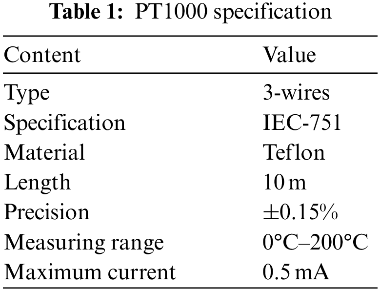
This study uses the Brother S500X1 milling machine in the experiment, as shown in Fig. 1. As for spindle temperature measurement, NI temperature input modules shown in Fig. 2 and PT1000 thick film platinum Resistance Temperature Detector (RTD) are used. The resistance of PT1000 is 1000 Ω at 0°C and increases as temperature rises. Its specifications are shown in Table 1: PT1000 Specification. And we measured the spindle’s five sensitive points and one ambient temperature shown in Fig. 2.

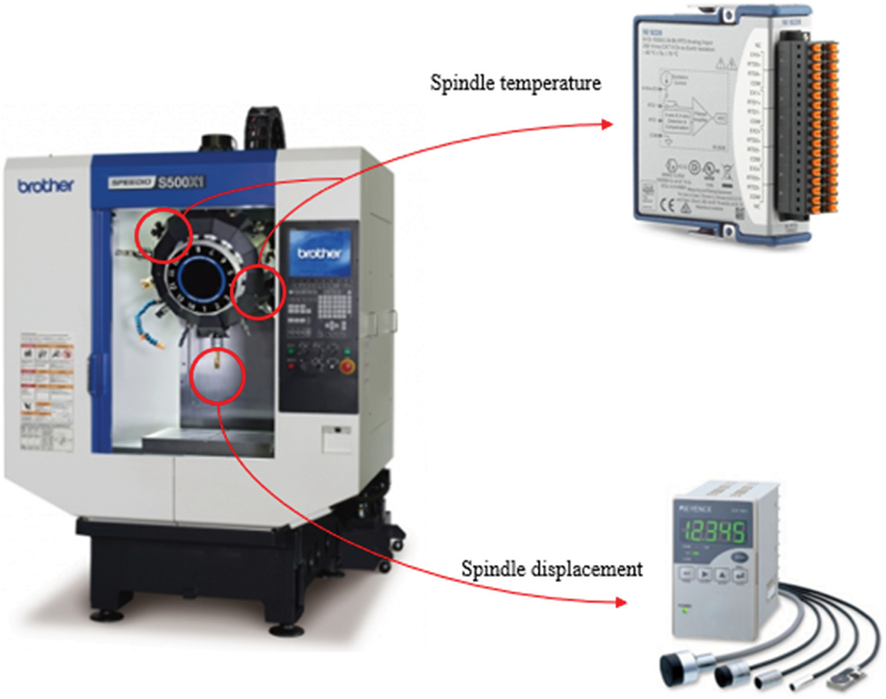
Figure 1: Layout of lab equipment

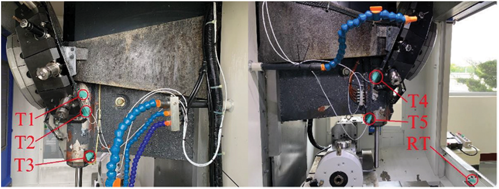
Figure 2: Sensitive temperature points

To measure the spindle displacement, EX-V02P Eddy Current Displacement Sensor and EX-110V displacement sensor (shown in Fig. 1) of KEYENCE are used in this study. The specifications of EX-110V are shown in Table 2.

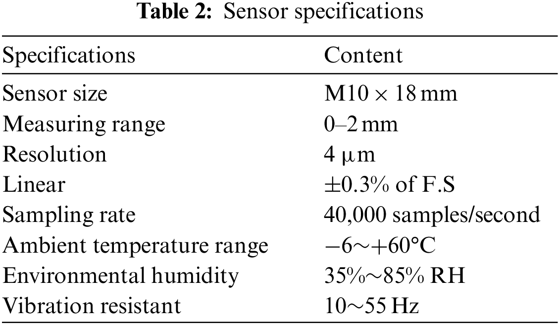
Fig. 3 shows how the eddy current displacement sensor is installed.

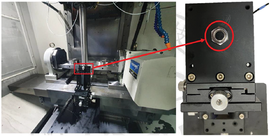
Figure 3: Installation location of eddy current displacement sensor

This study measures the spindle temperature and spindle displacement for different spindle speeds, i.e., 1000, 2000, 2500, 3000, 5000, 6000, 7500, and 9000, respectively. Data visualization is performed to facilitate the observation, as shown in Fig. 4.

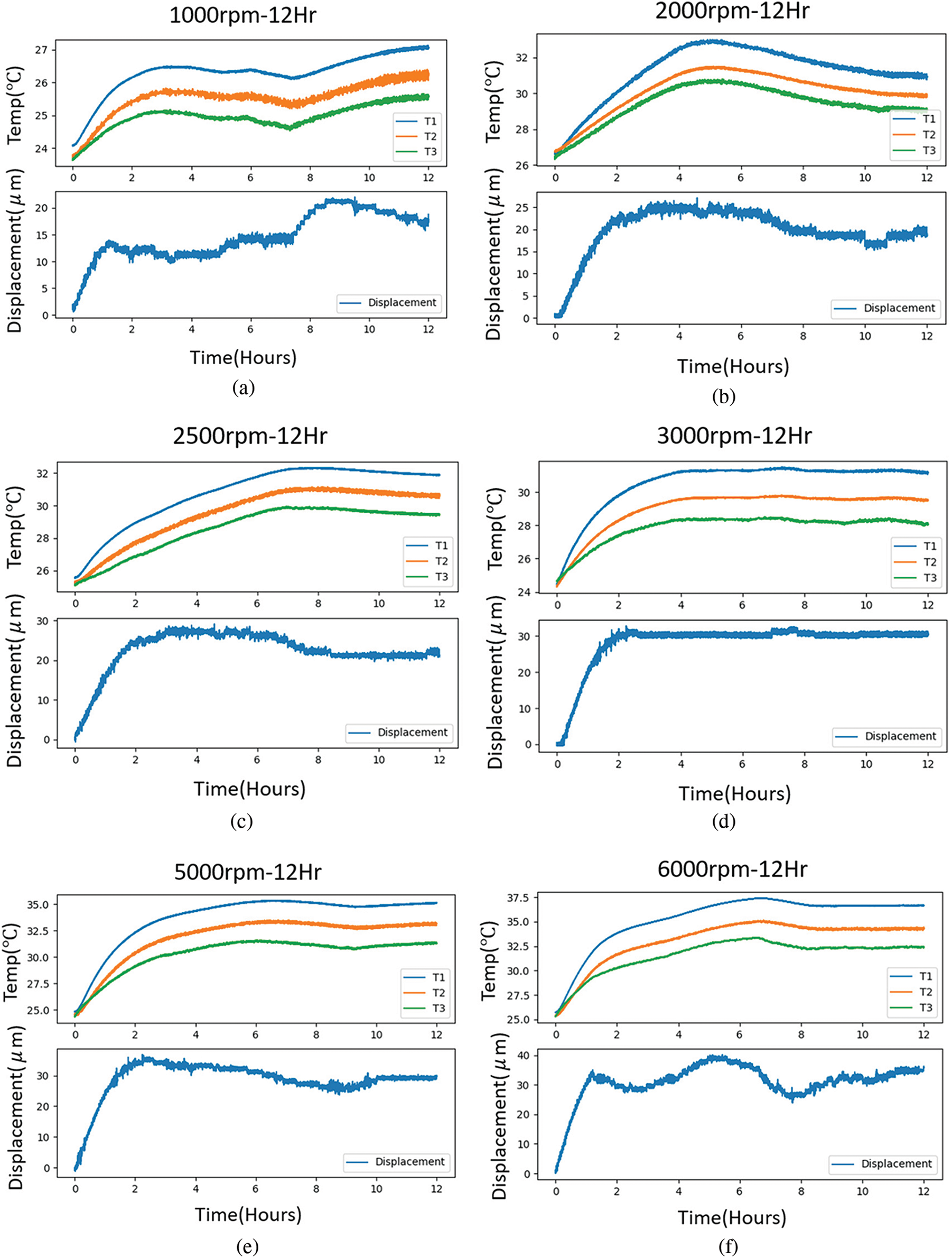
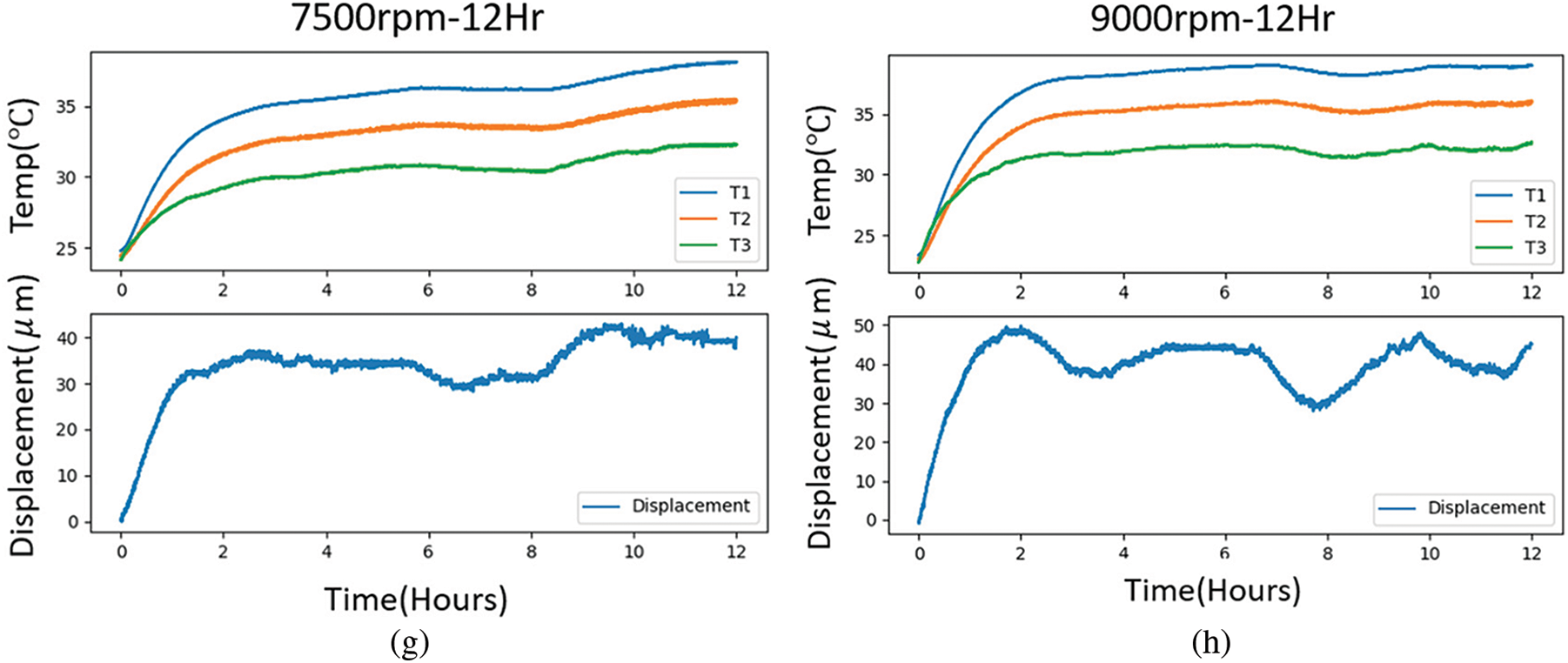
Figure 4: Data visualization: (a) 1000 rpm, (b) 2000 rpm, (c) 2500 rpm, (d) 3000 rpm, (e) 5000 rpm, (f) 6000 rpm, (g) 7500 rpm, (h) 9000 rpm

The figure above shows that the machine tool temperature rises and spindle displacement changes as the operating time of the spindle increases. Aiming to find the relationships between three variables, i.e., spindle temperature, displacement and time, this study uses LSTM neural network for modeling. A type of Recurrent Neural Network (RNN), LSTM is ideal for use on time-series data. It is used to model the relationships between the spindle temperature change and spindle displacement over a long period of time.

3  The Proposed Method

The model training architecture of this experiment is shown in Fig. 5. The goal is to establish the relationships between temperature rise and spindle displacement by using LSTM-SVM, which takes the temperature changes at multiple locations on the spindle and time sequence as input and then performs spindle thermal deformation prediction.

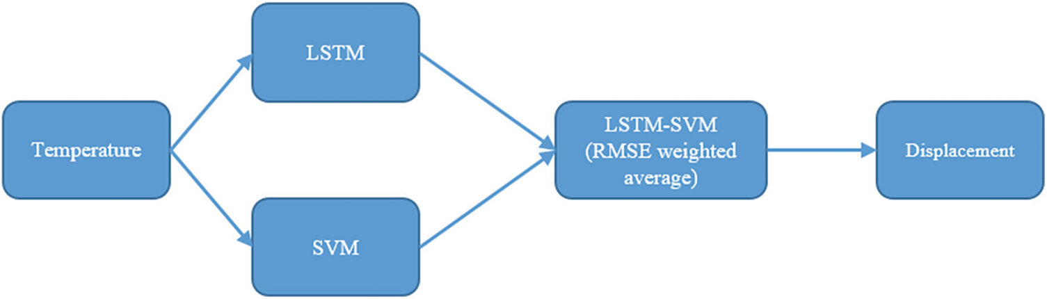
Figure 5: Model training architecture

Other algorithms are considered as well, including Long Short-Term Memory (LSTM) [27], one dimension Convolution Neural Network (CNN) [28], Support Vector Machine (SVM) [29], Decision Tree (DT) [30], Random Forest (RF) [31–33], Adaptive Boosting (AdaBoost) [34,35].

A type of Recurrent Neural Network (RNN), LSTM adopts a unique design that makes it ideal for processing and predicting time sequence related problems. It has been widely used in the studies of time sequence related problems. Fig. 6 shows the basic architecture of LSTM.

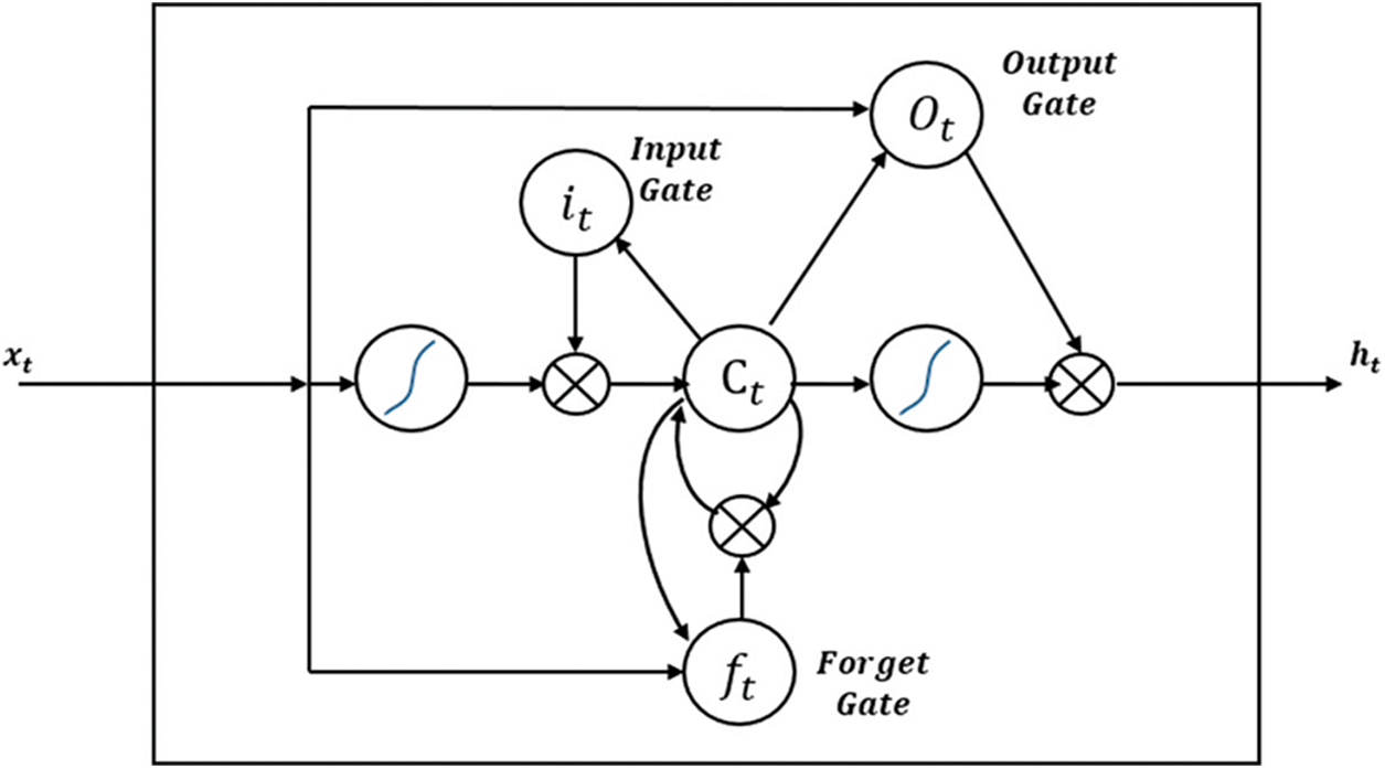
Figure 6: LSTM architecture1

LSTM is composed of four units, i.e., an Input Gate, an Output Gate, a Memory Cell and a Forget Gate. xt∈Rd denotes the input for the entire LSTM; it∈Rh denotes the input gate, which controls whether the data are used as input or not.

ft=σg(Wfxt+Ufht−1+bf)(1)

it=σg(Wixt+Uiht−1+bi)(2)

ot=σg(Woxt+Uoht−1+bo)(3)

ct=ft∘ct−1+it∘σc(Wcxt+Ucht−1+bc)(4)

ht=ot∘σh(ct)(5)

where  fi∈Rh denotes forget gate, which controls whether to clear the content of memory cell; ct∈Rh denotes memory cell, in which the calculated value is stored; ht∈Rh denotes the output of this LSTM.

The training effect will be affected when executing the model training under conditions where the data value scope is not evenly distributed. Before starting the model training, the data is normalized through the unification process so that the model can be trained under a more uniformly distributed data scope in order to achieve better prediction accuracy. The training data under different spindle speeds are combined, as shown in Fig. 7. Instead, if we want to know the 500th-second spindle displacement, we need the 496th to 500th-second spindle temperature. Every five sets of data under the same speed are combined into one set of input data for LSTM for training purposes.

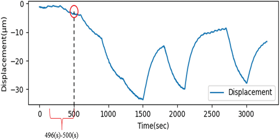
Figure 7: Time sequence

Convolution Neural Networks [36] (CNN) can be used for time sequence prediction problems. Traditionally developed for two-dimensional data, CNN can be used for modeling for single-variable time sequence problems as well, as shown in Fig. 8.

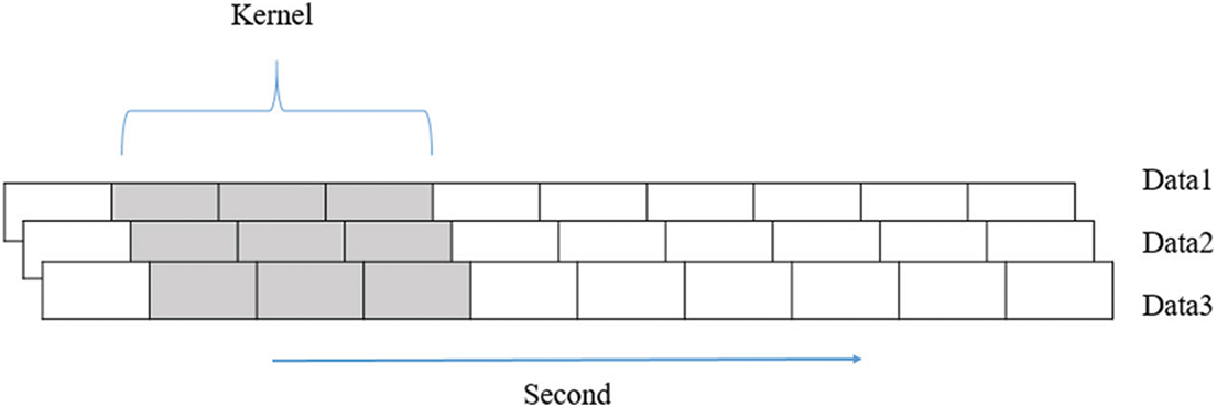
Figure 8: 1dimension convolution process

Support Vector Regression [37] (SVR) is a supervised machine learning algorithm for regression analysis. SVR model represents data as points in space. Such mapping divides the data in different categories as widely as possible by boundaries. Then the new data are mapped into the same space, and the prediction is performed based on which side of the boundary they are located, as shown in Fig. 9.

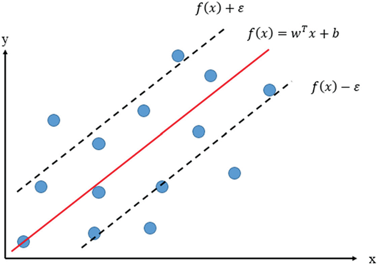
Figure 9: Support Vector Regression model

Decision Tree is composed of a decision diagram and possible outcomes. It is used to plan the route to reach the goal. Decision Tree is a tree structured decision-making tool, as shown in Fig. 10.

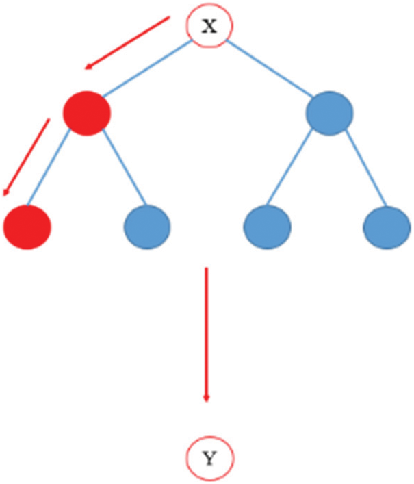
Figure 10: Decision Tree model

Random Forest consists of multiple decision trees. It works mainly based on a principle called the Bootstrap Aggregating algorithm, also known as Bagging. This algorithm uses sampling with replacements to create different data subsets, which are used to build the decision trees of the Ransom Forest, as shown in Fig. 11.

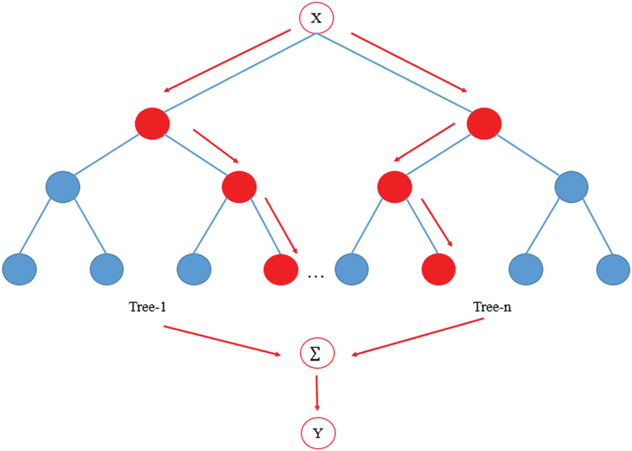
Figure 11: Random Forest model

Adaptive Boosting (AdaBoost) is a type of machine learning method. In the AdaBoost method, the samples misclassified by a classifier are used as training data for the next classifier. However, this method is quite sensitive to sound data and noisy data. Compared to other machine learning algorithms, AdaBoost is less prone to overfitting. AdaBoost may be a weak learner when used individually. If each learner performs better than a random guess, the final model will still converge and becomes a powerful learner, as shown in Fig. 12.

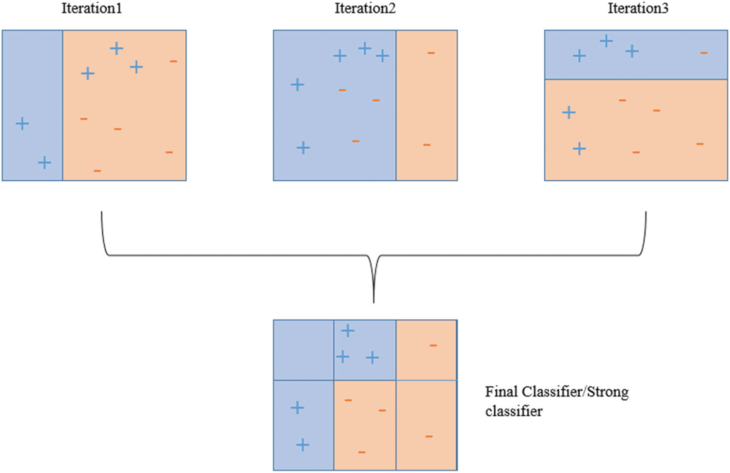
Figure 12: AdaBoost model

4  The Experimental Results

In this study, the LSTM-SVM model is trained with data of different speeds, i.e., 1000, 2500, 5000, 7500 and 9000 rpm. The model is then tested and verified with the data of 2000, 3000 and 6000 rpm. The prediction outcomes are shown in Fig. 13. Data visualization is applied to present the test data and actual data at various speeds.

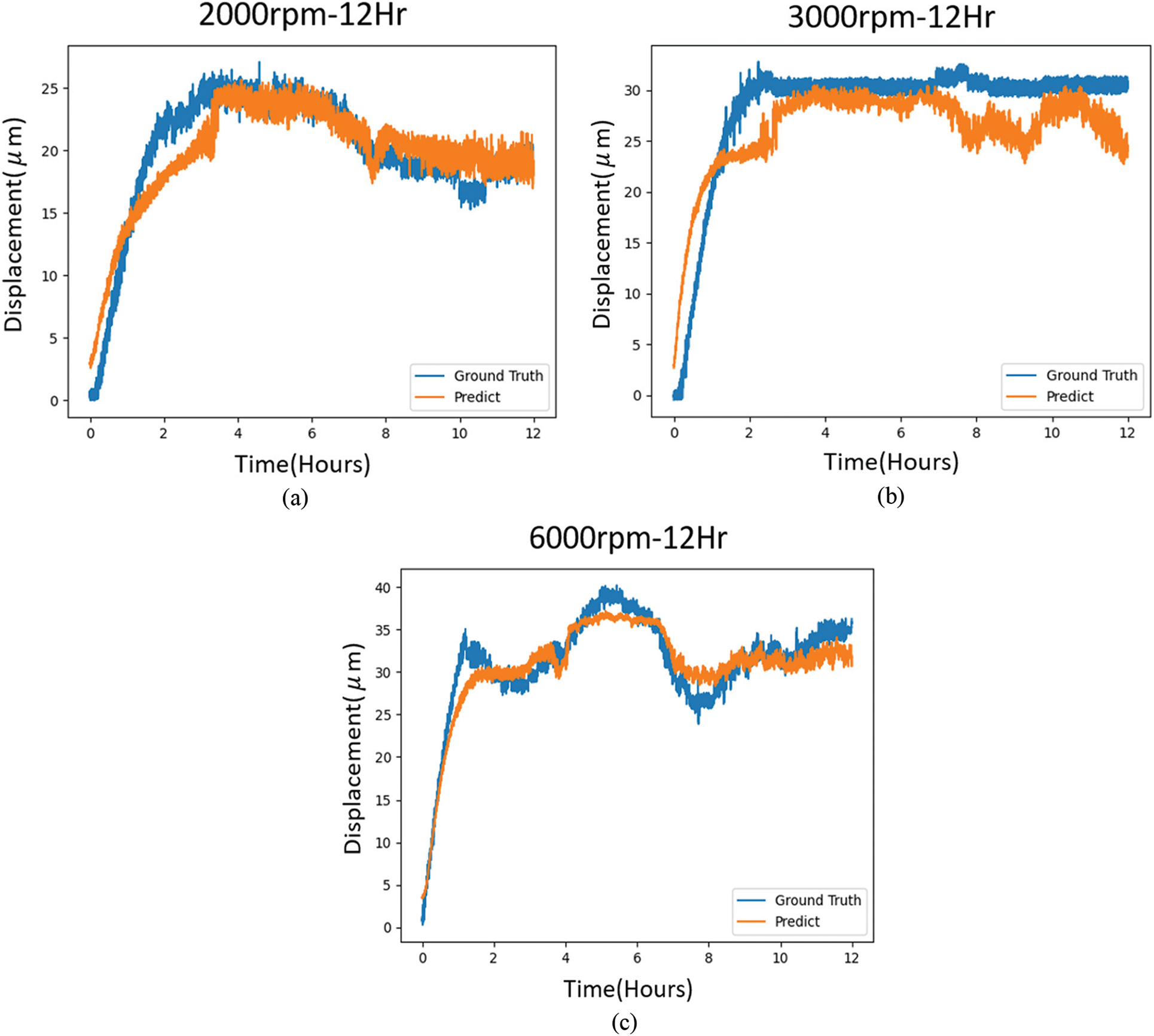
Figure 13: Prediction results visualization: (a) 2000 rpm (b) 3000 rpm (c) 6000 rpm

This study uses an LSTM-SVM model for spindle thermal displacement compensation prediction. The prediction results are compared with those made with LSTM, 1D CNN, SVR, DT, RF and AdaBoost models. Three evaluation methods, i.e., Mean Absolute Error (MAE), Mean Square Error (MSE), Root Mean Square Error (RMSE) and Coefficient of Determination (R2), are used to evaluate the prediction performance.

4.1 Mean Absolute Error Method

MAE is a type of loss function used in the regression model and is defined as the sum of the absolute values of the difference between target and predicted values. MAE measures the mean of prediction errors without considering the signs. MAE prevents the problem of positive and negative errors from being canceled out and, therefore, correctly reflects the degree of prediction errors. In Eq. (6), yi denotes the predicted value; y^i denotes the actual value; ei=|yi−y^i| denote absolute error.

MAE=1n∑i=1n|yi−y^i|=1n∑i=1n|ei|(6)

4.2 Mean-Square Error

MSE is the most commonly used loss function for regression. It is calculated as the square of the distance between the predicted and actual values, as shown in Eq. (7).

MSE=1n∑i=1n(yi−yi^)2(7)

4.3 Root-Mean-Square Error

RMSE is often used to describe the variance between values. RMSE often represents the error of model predictions or observed estimated values. Root Mean Square Deviation represents the standard deviation of prediction from the ground truth. The deviation is named residual when the difference is calculated between data samples. Root Mean Square Deviation is an appropriate measure of errors. According to the definition, RMSE is the square root of the mean of the square of the differences between actual values y  and predicted values y^, as shown in Eq. (8).

RMSE=1n∑i=1n(yi−yi^)2=MSE(8)

4.4 Coefficient of Determination

In statistics, R2 is used to measure the proportion of the variation in the dependent variable that can be explained by the independent variable(s). It indicates how well a prediction model is capable of explaining the proportion of variation. For simple linear regression, the coefficient of determination is the square of the sample correlation coefficients. In regression analysis and if other independent variables are added, the coefficient of determination is defined as the square of the coefficient of multiple correlations instead, as shown in Eq. (9).

R2=1−1n∑i=1n(yi−yi^)21n∑i=1n(yi−yi¯)2=1−MSE1n∑i=1n(yi−yi¯)2(9)

A type of Recurrent Neural Network (RNN), LSTM model is well-suited to process time sequence data and is thus appropriate for use in time sequence related prediction problems. However, LSTM has the problem of overfitting the training data. Applying dropout in LSTM is helpful in preventing overfitting and improving prediction performance. In the LSTM model of this study, the activation function is composed of three layers of the sigmoid function, each with 20 cells. The dropout is set to 0.2. Adaptive Moment Estimation (Adam) is used as the optimizer for model training. The results show that this LSTM has achieved performance in terms of MAEs of 2.66, 2.42, and 2.16, RMSEs of 3.31, 3.75 and 2.78 and R2 of 0.59, 0.66, and 0.78, as shown in Fig. 14.

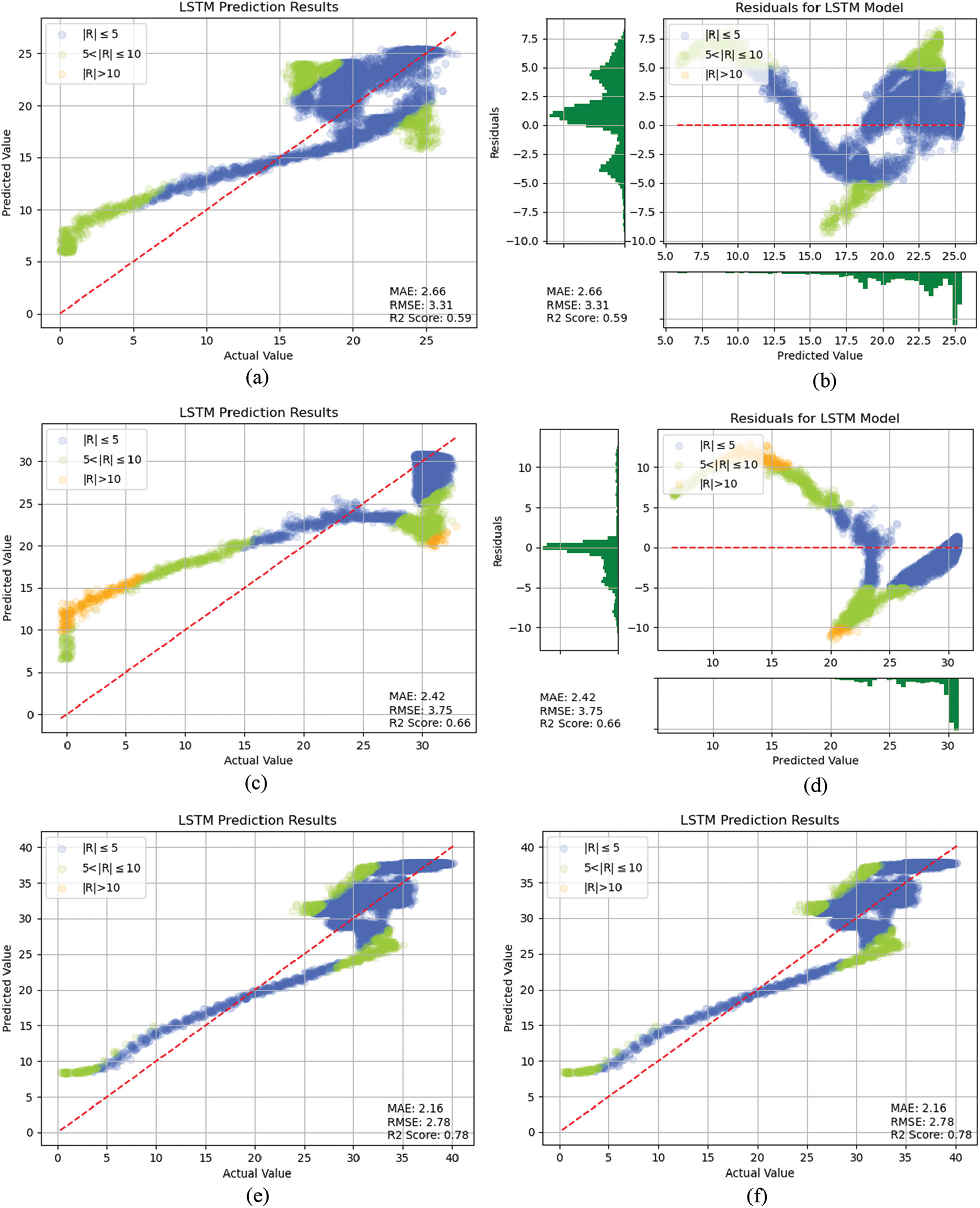
Figure 14: LSTM prediction result: (a) 2000 rpm comparison of actual and predicted values, (b) 2000 rpm residual plot, (c) 3000 rpm comparison of actual and predicted values, (d) 3000 rpm residual plot, (e) 6000 rpm comparison of actual and predicted values, (f) 6000 rpm residual plot

The 1D CNN has a convolution hidden layer that operates over a 1D sequence. A convolutional layer has 32 filters. The kernel size is set to 3. Then a pooling layer of pool size 2 is applied after the convolutional layer. The goal is to down sample the data from the convolution layer by extracting important features from the data. A Flatten function is used to flatten the data. A two-layer dropout is applied with dropout = 0.1. The activation function is Rectified Linear Unit (Relu) [38]. Adam [39] is used as the optimizer for model training. Fig. 15 shows the prediction performance delivered by the CNN, i.e., MAEs of 3.27, 6.13 and 2.58, RMSEs of 3.77, 6.54 and 3.08, and R2 of 0.47, −0.04 and 0.73. The SVR operates with RBF kernel, gamma = 0.1 and C = 1e3. Fig. 16 shows the prediction performance delivered, i.e., MAEs of 1.65, 4.1 and 1.99, RMSEs of 2.02, 4.55 and 2.36, and R2 of 0.85, 0.5 and 0.85. The operational strategy of using the Decision Tree algorithm is to set the following parameters; criterion, MSE; sample number of internal node, 2; sample number of leave node, 1. Fig. 17 shows the prediction performance delivered, i.e., MAEs of 3.64, 4.73 and 3.06, RMSEs of 4.43, 5.61 and 3.91, and R2 of 0.27, 0.24 and 0.57. The operational strategy of using the Random Forest algorithm is to set the following parameters: the number of forests, 100; split function, MSE; sample number of internal node, 2; sample number of leave node, 1. Fig. 18 shows the prediction performance delivered, i.e., MAEs of 1.86, 3.82 and 2.62, RMSEs of 2.16, 4.08 and 3.27, and R2 of 0.83, 0.6 and 0.7. The operational strategy of using the AdaBoost algorithm is to set the number of estimators and the weight of each classifier to 50 and 1, respectively. Fig. 19 shows the prediction performance delivered, i.e., MAEs of 1.85, 4.15 and 2.77, RMSEs of 2.2, 4.35 and 3.29, and R2 of 0.82, 0.54 and 0.7.

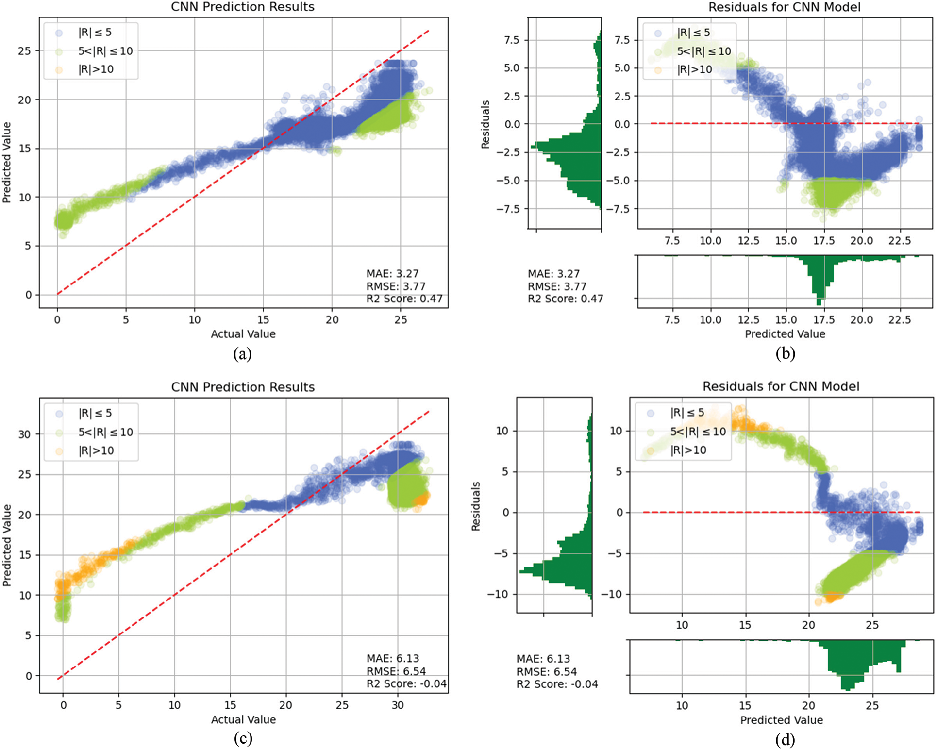
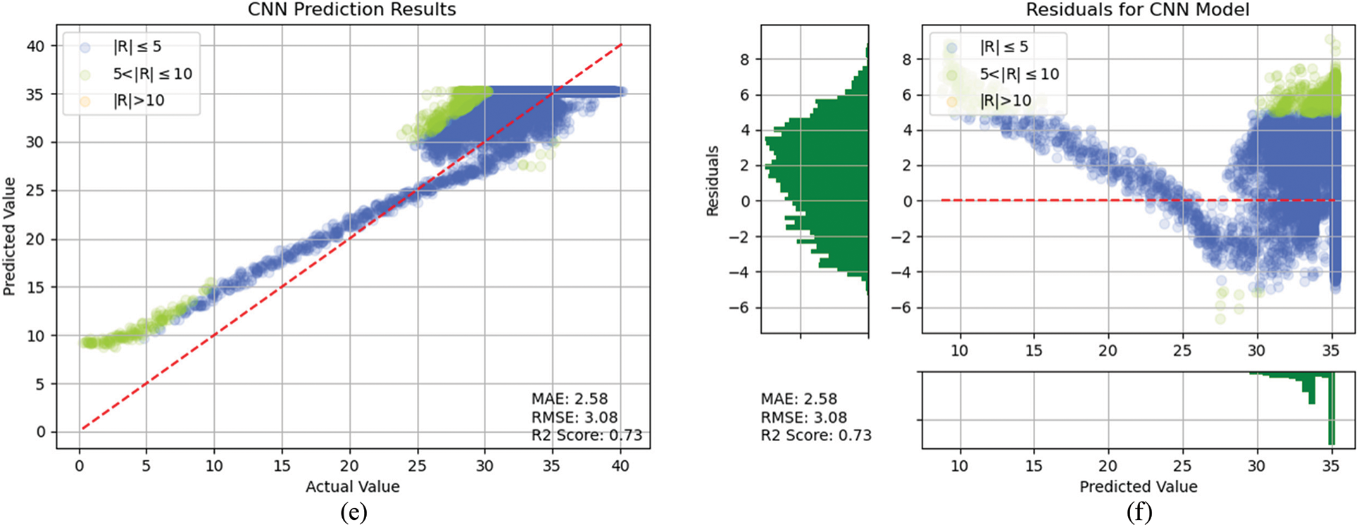
Figure 15: 1D CNN prediction result: (a) 2000 rpm comparison of actual and predicted values, (b) 2000 rpm residual plot, (c) 3000 rpm comparison of actual and predicted values, (d) 3000 rpm residual plot, (e) 6000 rpm comparison of actual and predicted values, (f) 6000 rpm residual plot

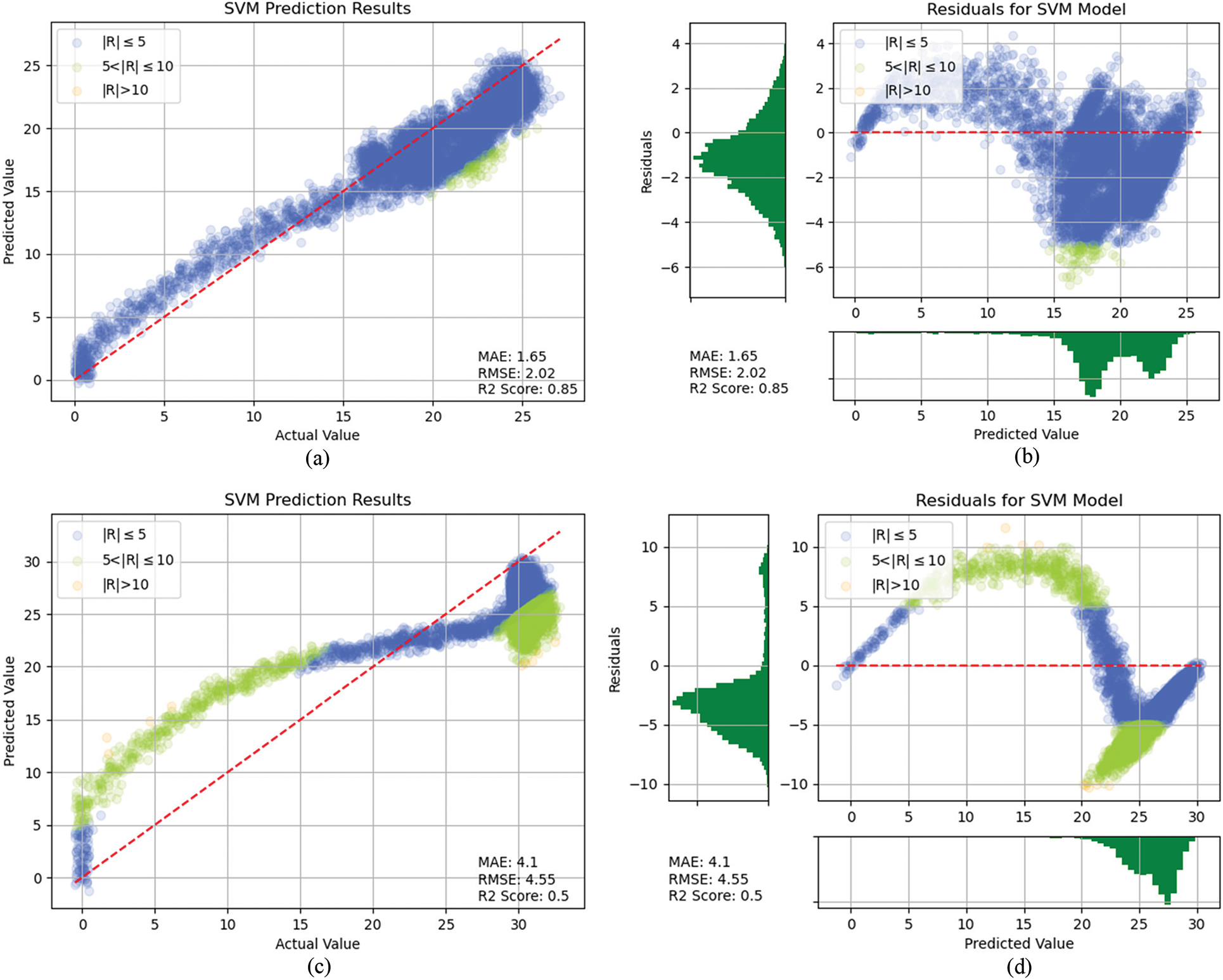
Figure 16: SVM prediction result: (a) 2000 rpm comparison of actual and predicted values, (b) 2000 rpm residual plot, (c) 3000 rpm comparison of actual and predicted values, (d) 3000 rpm residual plot, (e) 6000 rpm comparison of actual and predicted values, (f) 6000 rpm Residual plot

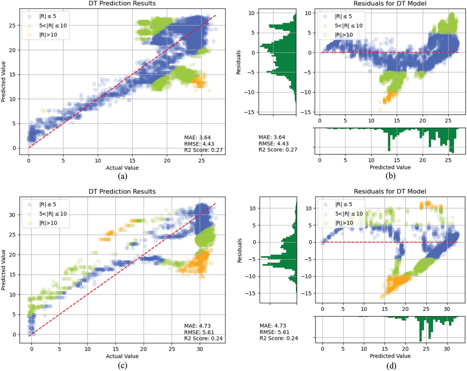
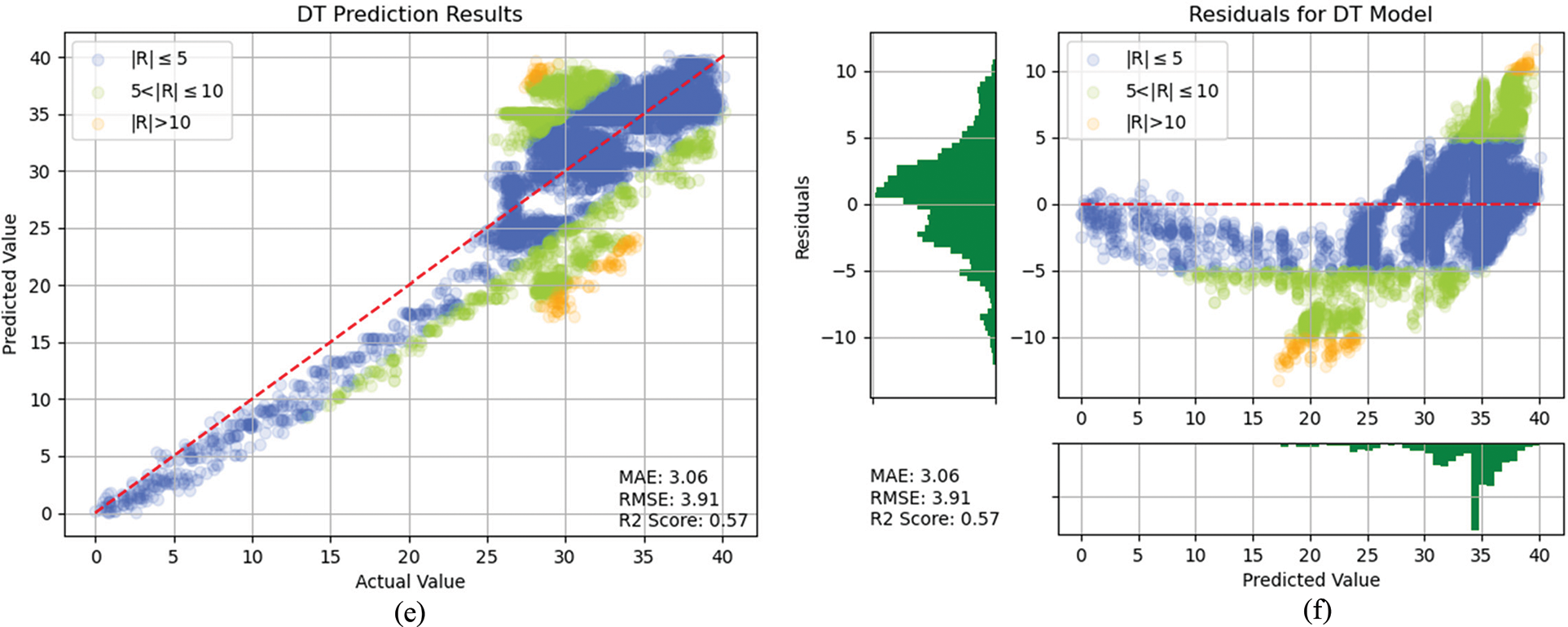
Figure 17: Decision tree prediction result: (a) 2000 rpm comparison of actual and predicted values, (b) 2000 rpm residual plot, (c) 3000 rpm comparison of actual and predicted values, (d) 3000 rpm residual plot, (e) 6000 rpm comparison of actual and predicted values, (f) 6000 rpm residual plot

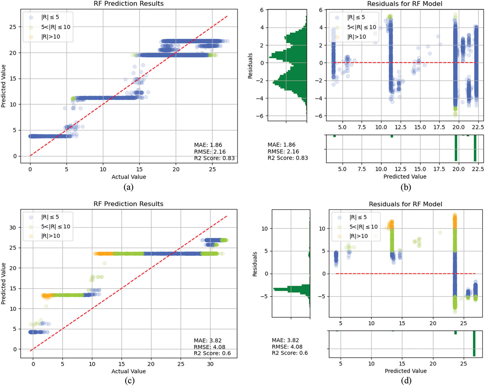
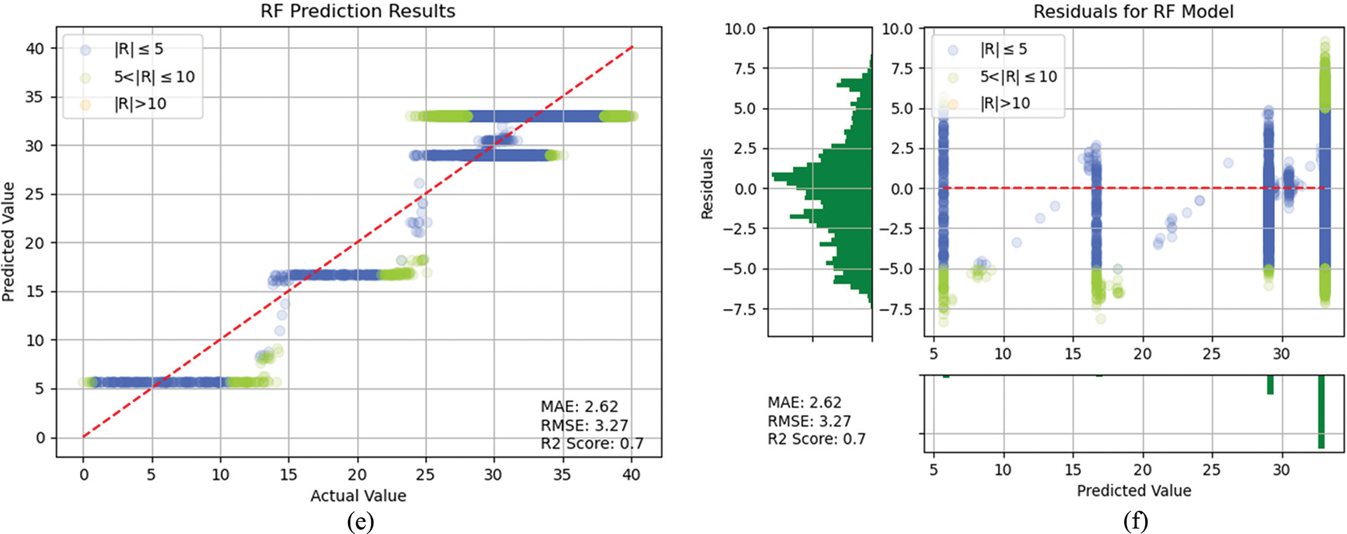
Figure 18: Random forest prediction result: (a) 2000 rpm comparison of actual and predicted values, (b) 2000 rpm residual plot, (c) 3000 rpm comparison of actual and predicted values, (d) 3000 rpm residual plot, (e) 6000 rpm comparison of actual and predicted values, (f) 6000 rpm residual plot

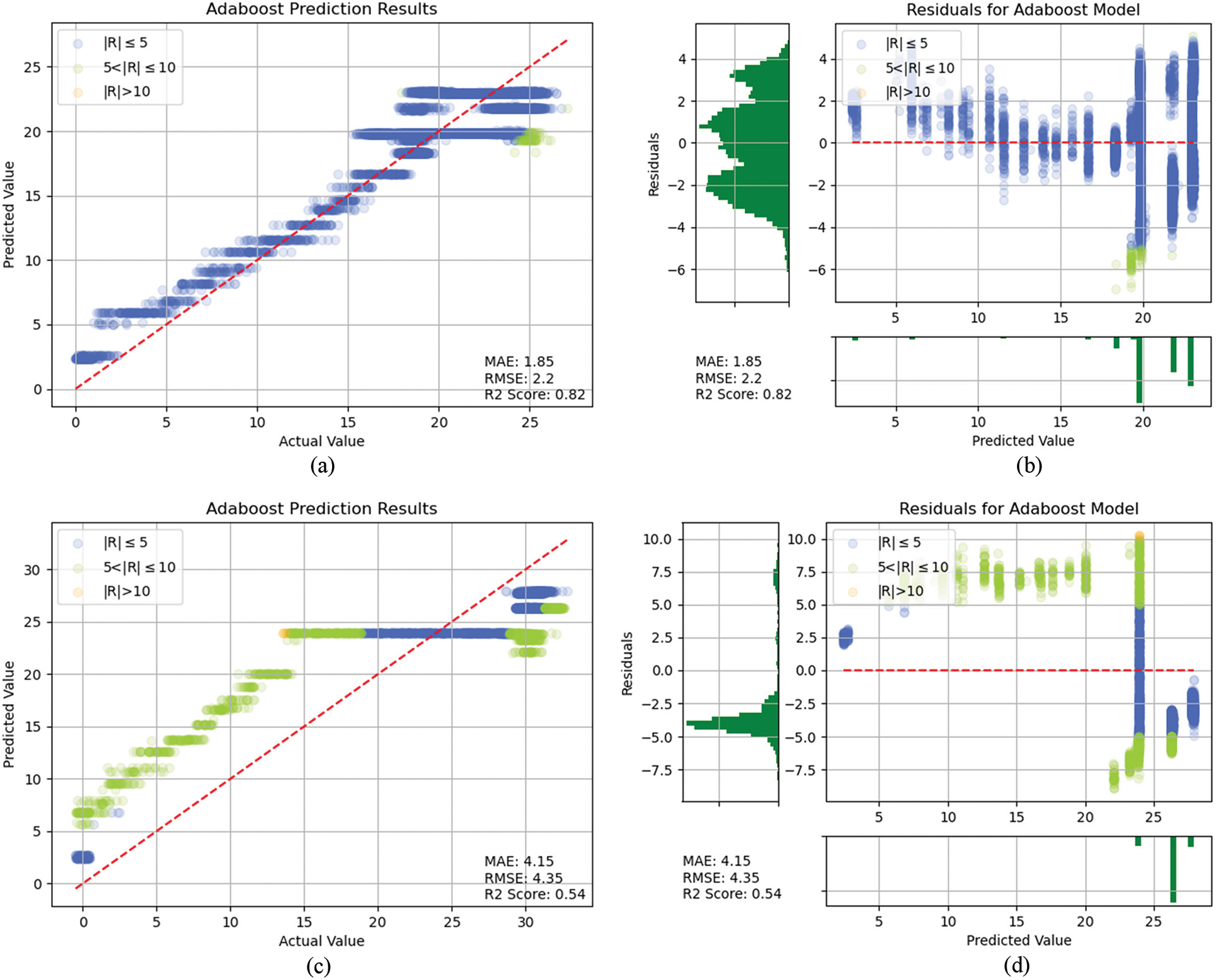
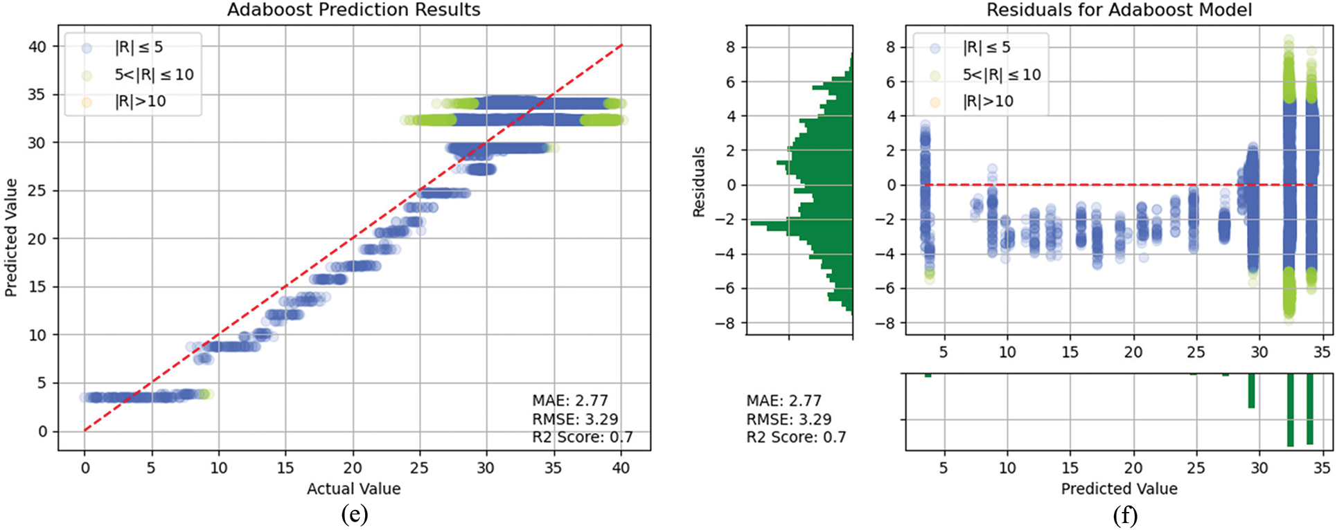
Figure 19: AdaBoost prediction result: (a) 2000 rpm comparison of actual and predicted values, (b) 2000 rpm residual plot, (c) 3000 rpm comparison of actual and predicted values, (d) 3000 rpm residual plot, (e) 6000 rpm comparison of actual and predicted values, (f) 6000 rpm residual plot

The above results show that the LSTM and the SVM [40–42]-based ensemble models achieve the best prediction error performance. From the above, we see that the rest of the other points are poorly distributed, except for LSTM, SVM, DT and CNN, so they will not be precluded. By comparing the R2 of the aforesaid four points, it is found that a negative value is presented when CNN is operating up to 3000 rpm and the R2 of DT is also too low. Therefore, LSTM and SVM are selected for use as the basic model of the ensemble model during the research. The two are therefore combined into one hybrid LSTM-SVM model. The LSTM-SVM model operates as follows. The LSTM and SVM models have trained again separately with the test data and corresponding RMSEs are obtained. The weights of predicted values of the two models are determined based on the RMSEs. The weighted predicted values are added up as the final results. The final results are calculated as shown in Eq. (9), where Pfinal denotes the final results;Plstm denotes the predicted values of LSTM model; Psvm denotes the predicted values of SVM model; LSTMrmse denotes the RMSE obtained from the LSTM model trained with training data; SVMrmse denotes the RMSE obtained from the SVM model trained with training data. In other words, the better model is given a higher weight. In the LSTM, the sigmoid function is used in all three layers. Each layer has 20 cells and dropout rate is 0.2. Adam is used as the optimizer for model training. The SVR uses RBF kernel, with gamma = 0.1 and C = 1e3. The weighted mean of the two predicted values is then calculated. Fig. 20 shows the prediction performance delivered, i.e., MAEs 1.64, 3.22 and 1.67, RMSEs of 2.13, 3.91 and 2.04, and R2 of 0.83, 0.63 and 0.88.

Pfinal=Plstm×SVMrmseLSTMrmse+SVMrmse+Psvm×LSTMrmseLSTMrmse+SVMrmse(10)

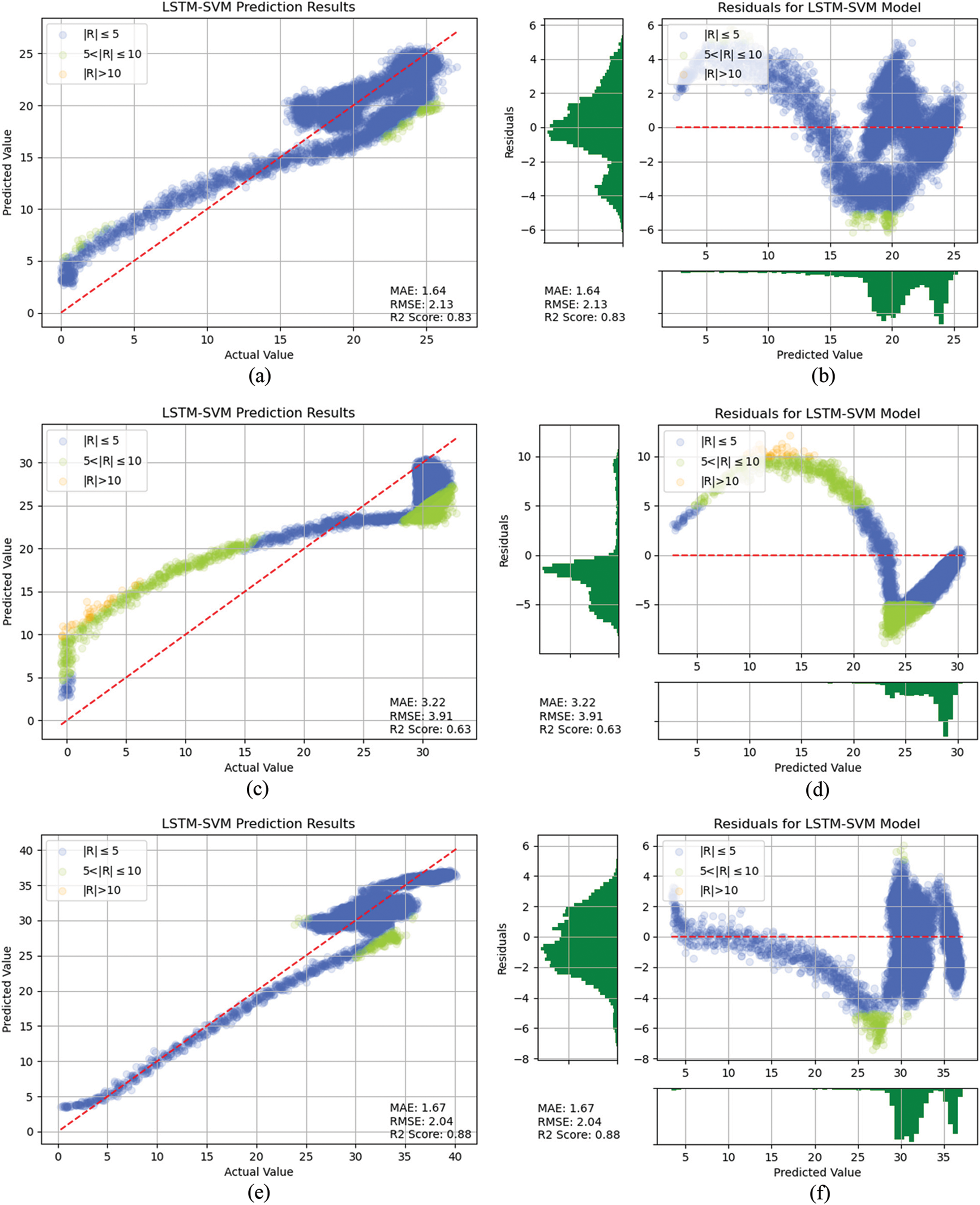
Figure 20: LSTM-SVM prediction result: (a) 2000 rpm comparison of actual and predicted values, (b) 2000 rpm residual plot, (c) 3000 rpm comparison of actual and predicted values, (d) 3000 rpm residual plot, (e) 6000 rpm comparison of actual and predicted values, (f) 6000 rpm residual plot

The RMSEs obtained from different models are tabulated for ease of comparison. Table 3 shows that the LSTM-SVM model used in this study is superior to the others in terms of prediction performance. The variance of errors across predictions is constant. The model is robust and the distribution of RSMEs is even under all speeds.

5  Conclusion

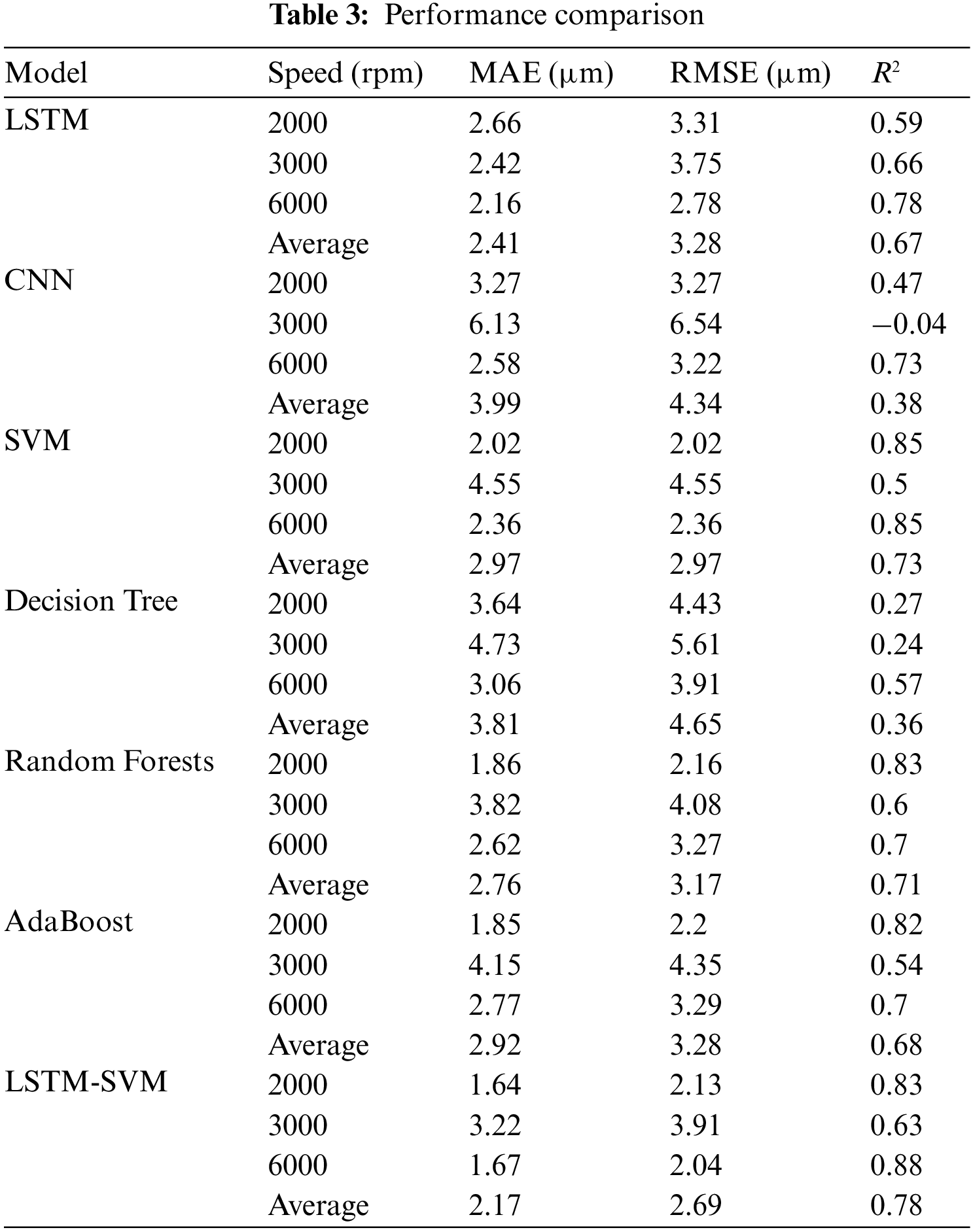
The above experiment results show that LSTM and SVM models achieve better results in spindle thermal displacement prediction. The experiment results show that when the SVM prediction model is used alone, the RSMEs of the predicted values under 3000 rpm of spindle speed are higher than those under 2000 and 6000 rpm. Also, when the LSTM prediction model is used alone, the RSMEs under different speeds are quite close. In addition, the LSTM outperforms SVM in prediction in only a few cases. The two models are therefore combined into one hybrid LSTM-SVM model. The weighted mean of the two predicted values is then calculated through the assignment of weights. The experiment demonstrates that this hybrid LSTM-SVM model has successfully lowered the RMSEs of prediction error to 2.13, 3.91 and 2.04. The overall mean RMSEs is 2.69, which is better than LSTM and SVM models, i.e., 3.28 and 2.97, respectively. The LSTM-SVM Spindle, thermal displacement prediction model, selected for this research not only elevates the machining accuracy of the machine tools but also saves the consumption of time and energy required for heating up the machine tools. To acquire more accurate verification results, it also allows us to collect other types of revolutions as well as accurate temperature and thermal displacement data in order to develop a more effective model. As a result, higher universality can be achieved in the long run.

Funding Statement: This work was supported by the Ministry of Science and Technology, Taiwan, under Grant MOST 110-2218-E-194-010. This work was financially partially supported by the Advanced Institute of Manufacturing with High-Tech Innovations (AIM-HI) from the Featured Areas Research Center Program within the Framework of the Higher Education Sprout Project by the Ministry of Education (MOE) in Taiwan.

Conflicts of Interest: The authors declare that they have no conflicts of interest to report regarding the present study.

References

1. Huchel, M., Krause, T. C., Lugowski, T., Leeb, S. B., Helsen, J. (2021). Chasing the Cut: A measurement approach for machine tool condition monitoring. IEEE Transactions on Instrumentation and Measurement, 70, 1–10. https://doi.org/10.1109/TIM.2020.3047939 [Google Scholar] [CrossRef]

2. Ding, X., He, Q. (2017). Energy-fluctuated multiscale feature learning with deep ConvNet for intelligent spindle bearing fault diagnosis. IEEE Transactions on Instrumentation and Measurement, 66(8), 1926–1935. https://doi.org/10.1109/TIM.2017.2674738 [Google Scholar] [CrossRef]

3. Ibaraki, S., Okumura, R. (2021). A machining test to evaluate thermal influence on the kinematics of a five-axis machine tool. International Journal of Machine Tools and Manufacture, 163, 103702. https://doi.org/10.1016/j.ijmachtools.2021.103702 [Google Scholar] [CrossRef]

4. Li, Y., Zhao, W., Lan, S., Ni, J., Wu, W. et al. (2015). A review on spindle thermal error compensation in machine tools. International Journal of Machine Tools and Manufacture, 95(99), 20–38. https://doi.org/10.1016/j.ijmachtools.2015.04.008 [Google Scholar] [CrossRef]

5. Mayr, J., Jedrzejewski, J., Uhlmann, E., Donmez, M. A., Knapp, W. et al. (2012). Thermal issues in machine tools. CIRP Annals, 61(2), 771–791. https://doi.org/10.1016/j.cirp.2012.05.008 [Google Scholar] [CrossRef]

6. Liu, K., Liu, Y., Sun, M., Li, X., Wu, Y. (2016). Spindle axial thermal growth modeling and compensation on CNC turning machines. The International Journal of Advanced Manufacturing Technology, 87(5–8), 2285–2292. https://doi.org/10.1007/s00170-016-8593-5 [Google Scholar] [CrossRef]

7. Ramesh, R., Mannan, M., Poo, A. (2000). Error compensation in machine tools—A review. International Journal of Machine Tools and Manufacture, 40(9), 1257–1284. https://doi.org/10.1016/S0890-6955(00)00010-9 [Google Scholar] [CrossRef]

8. Kryzhanivskyy, V., M’Saoubi, R., Ståhl, J. E., Bushlya, V. (2019). Tool–chip thermal conductance coefficient and heat flux in machining: Theory, model and experiment. International Journal of Machine Tools and Manufacture, 147, 103468. https://doi.org/10.1016/j.ijmachtools.2019.103468 [Google Scholar] [CrossRef]

9. Abdulshahed, A. M., Longstaff, A. P., Fletcher, S. (2015). The application of ANFIS prediction models for thermal error compensation on CNC machine tools. Applied Soft Computing, 27, 158–168. https://doi.org/10.1016/j.asoc.2014.11.012 [Google Scholar] [CrossRef]

10. Weng, L., Gao, W., Zhang, D., Huang, T., Liu, T. et al. (2021). Analytical modelling method for thermal balancing design of machine tool structural components. International Journal of Machine Tools and Manufacture, 164, 103715. https://doi.org/10.1016/j.ijmachtools.2021.103715 [Google Scholar] [CrossRef]

11. Liu, T., Gao, W., Zhang, D., Zhang, Y., Chang, W. et al. (2017). Analytical modeling for thermal errors of motorized spindle unit. International Journal of Machine Tools and Manufacture, 112, 53–70. https://doi.org/10.1016/j.ijmachtools.2016.09.008 [Google Scholar] [CrossRef]

12. Li, Y., Zhao, W. (2012). Axial thermal error compensation method for the spindle of a precision horizontal machining center. 2012 IEEE International Conference on Mechatronics and Automation, pp. 2319–2323. Chengdu, China. https://doi.org/10.1109/ICMA.2012.6285706. [Google Scholar] [CrossRef]

13. Chen, S. H., Tsai, Y. L. (2016). The machine-tool temperature variation measurement and compensation using regression analysis method. 2016 International Conference on Advanced Materials for Science and Engineering (ICAMSE), pp. 673–676. Tai-Chung, Taiwan. https://doi.org/10.1109/ICAMSE.2016.7840292 [Google Scholar] [CrossRef]

14. Wang, K. (2006). Thermal error modeling of a machining center using grey system theory and adaptive network-based fuzzy inference system. 2006 IEEE Conference on Cybernetics and Intelligent Systems, pp. 1–6. Taichung, Taiwan. https://doi.org/10.1109/ICCIS.2006.252254 [Google Scholar] [CrossRef]

15. Li, Q., Li, H. (2019). A general method for thermal error measurement and modeling in CNC machine tools’ spindle. The International Journal of Advanced Manufacturing Technology, 103(5–8), 2739–2749. https://doi.org/10.1007/s00170-019-03665-7 [Google Scholar] [CrossRef]

16. Zhang, Y., Yang, J., Jiang, H. (2012). Machine tool thermal error modeling and prediction by grey neural network. The International Journal of Advanced Manufacturing Technology, 59(9–12), 1065–1072. https://doi.org/10.1007/s00170-011-3564-3 [Google Scholar] [CrossRef]

17. Wu, C. Y., Xiang, S. T., Xiang, W. S. (2021). Spindle thermal error prediction approach based on thermal infrared images: A deep learning method. Journal of Manufacturing Systems, 59, 67–80. https://doi.org/10.1016/j.jmsy.2021.01.013 [Google Scholar] [CrossRef]

18. Kang, Y., Chang, C. W., Huang, Y., Hsu, C. L., Nieh, I. F. (2007). Modification of a neural network utilizing hybrid filters for the compensation of thermal deformation in machine tools. International Journal of Machine Tools and Manufacture, 47(2), 376–387. https://doi.org/10.1016/j.ijmachtools.2006.03.007 [Google Scholar] [CrossRef]

19. Wu, H., Zhang, H. T., Guo, Q. J., Wang, X. S., Yang, J. G. (2008). Thermal error optimization modeling and real-time compensation on a CNC turning center. Journal of Materials Processing Technology, 207(1–3), 172–179. https://doi.org/10.1016/j.jmatprotec.2007.12.067 [Google Scholar] [CrossRef]

20. Liu, J., Ma, C., Gui, H., Wang, S. (2021). Thermally-induced error compensation of spindle system based on long short term memory neural networks. Applied Soft Computing, 102, 107094. https://doi.org/10.1016/j.asoc.2021.107094 [Google Scholar] [CrossRef]

21. Liang, Y. C., Li, W. D., Lou, P., Hu, J. M. (2020). Thermal error prediction for heavy-duty CNC machines enabled by long short-term memory networks and fog-cloud architecture. Journal of Manufacturing Systems, 62, 950–963. https://doi.org/10.1016/j.jmsy.2020.10.008 [Google Scholar] [CrossRef]

22. Shi, H., Jiang, C., Yan, Z., Tao, T., Mei, X. (2020). Bayesian neural network–based thermal error modeling of feed drive system of CNC machine tool. The International Journal of Advanced Manufacturing Technology, 108(9–10), 3031–3044. https://doi.org/10.1007/s00170-020-05541-1 [Google Scholar] [CrossRef]

23. Li, G., Ke, H., Li, C., Li, B. (2020). Thermal error modeling of feed axis in machine tools using particle swarm optimization-based generalized regression neural network. Journal of Computing and Information Science in Engineering, 20(2). https://doi.org/10.1115/1.4045292 [Google Scholar] [CrossRef]

24. Rauf, H. T., Gao, J., Almadhor, A., Arif, M., Nafis, M. T. (2021). Enhanced bat algorithm for COVID-19 short-term forecasting using optimized LSTM. Soft Computing, 25(20), 12989–12999. https://doi.org/10.1007/s00500-021-06075-8 [Google Scholar] [PubMed] [CrossRef]

25. Usharani, B. (2022). ILF-LSTM: Enhanced loss function in LSTM to predict the sea surface temperature. Soft Computing. https://doi.org/10.1007/s00500-022-06899-y [Google Scholar] [CrossRef]

26. Bao, T., Zaidi, S. A. R., Xie, S., Yang, P., Zhang, Z. Q. (2021). A CNN-LSTM hybrid model for wrist kinematics estimation using surface electromyography. IEEE Transactions on Instrumentation and Measurement, 70, 1–9. https://doi.org/10.1109/TIM.2020.3036654 [Google Scholar] [CrossRef]

27. Hochreiter, S., Schmidhuber, J. (1997). Long short-term memory. Neural Computation, 9(8), 1735–1780. https://doi.org/10.1162/neco.1997.9.8.1735 [Google Scholar] [PubMed] [CrossRef]

28. Lecun, Y., Bottou, L., Bengio, Y., Haffner, P. (1998). Gradient-based learning applied to document recognition. Proceedings of the IEEE, 86(11), 2278–2324. https://doi.org/10.1109/5.726791 [Google Scholar] [CrossRef]

29. Cortes, C., Vapnik, V. (1995). Support-vector networks. Machine Learning, 20(3), 273–297. https://doi.org/10.1007/BF00994018 [Google Scholar] [CrossRef]

30. Quinlan, J. R. (1986). Induction of decision trees. Machine Learning, 1(1), 81–106. https://doi.org/10.1007/BF00116251 [Google Scholar] [CrossRef]

31. Subha, S., Baghavathi Priya, S. (2023). Prediction model for a good learning environment using an ensemble approach. Computer Systems Science and Engineering, 44(3), 2081–2093. https://doi.org/10.32604/csse.2023.028451 [Google Scholar] [CrossRef]

32. Muhammad, F., Khan, B., Naseem, R., Asiri, A. A., Alshamrani, H. A. et al. (2023). Liver ailment prediction using random forest model. Computers, Materials & Continua, 74(1), 1049–1067. https://doi.org/10.32604/cmc.2023.032698 [Google Scholar] [CrossRef]

33. Ho, T. K., Random decision forests. Proceedings of 3rd International Conference on Document Analysis and Recognition, vol. 1, pp. 278–282. Montreal, QC, Canada. https://doi.org/10.1109/ICDAR.1995.598994 [Google Scholar] [CrossRef]

34. Rojas, R. (2009). AdaBoost and the super bowl of classifiers A tutorial introduction to adaptive boosting. Technical Report, Freie University, Berlin. https://www.cmi.ac.in/~madhavan/courses/dmml2022/literature/rojas-adaboost.pdf [Google Scholar]

35. Bagkur, C., Guler, E., Kaymakamzade, B., Hincal, E., Suer, K. (2022). Near future perspective of esbl-producing klebsiella pneumoniae strains using mathematical modeling. Computer Modeling in Engineering & Sciences, 130(1), 111–132. https://doi.org/10.32604/cmes.2022.016957 [Google Scholar] [CrossRef]

36. Ketu, S., Mishra, P. K. (2022). India perspective: CNN-LSTM hybrid deep learning model-based COVID-19 prediction and current status of medical resource availability. Soft Computing, 26(2), 645–664. https://doi.org/10.1007/s00500-021-06490-x [Google Scholar] [PubMed] [CrossRef]

37. Tabari, M. M. R., Sanayei, H. R. Z. (2019). Prediction of the intermediate block displacement of the dam crest using artificial neural network and support vector regression models. Soft Computing, 23(19), 9629–9645. https://doi.org/10.1007/s00500-018-3528-8 [Google Scholar] [CrossRef]

38. Xu, B., Wang, N., Chen, T., Li, M. (2015). Empirical evaluation of rectified activations in convolutional network. https://arxiv.org/pdf/1505.00853.pdf [Google Scholar]

39. Kingma, D. P., Ba, J. L. (2015). ADAM: A method for stochastic optimization. 3rd International Conference for Learning Representations, pp. 1–15. San Diego, USA. [Google Scholar]

40. Rodan, A., Sheta, A. F., Faris, H. (2017). Bidirectional reservoir networks trained using SVM + privileged information for manufacturing process modeling. Soft Computing, 21(22), 6811–6824. https://doi.org/10.1007/s00500-016-2232-9 [Google Scholar] [CrossRef]

41. Sharma, N., Haq, M. A., Dahiya, P. K., Marwah, B. R., Lalit, R. et al. (2023). Deep learning and SVM-based approach for Indian licence plate character recognition. Computers, Materials & Continua, 74(1881–895. https://doi.org/10.32604/cmc.2023.027899 [Google Scholar] [CrossRef]

42. Dutta, N., Kaliannan, P., Shanmugam, P. (2023). SVM algorithm for vibration fault diagnosis in centrifugal pump. Intelligent Automation & Soft Computing, 35(3), 2997–3020. https://doi.org/10.32604/iasc.2023.028704 [Google Scholar] [CrossRef]