
 Submit a Paper
 Propose a Special lssue
 Open Access
ARTICLE

Pedestrian and Vehicle Detection Based on Pruning YOLOv4 with Cloud-Edge Collaboration
1
School of Computer Science and Engineering, Huizhou University, Huizhou, 516007, China
2
School of Computer Science and Engineering, South China University of Technology, Guangzhou, 510006, China
3
School of Computer Science and Technology, South China Normal University, Guangzhou, 510631, China
4
Department of New Network Technologies, Peng Cheng Laboratory, Shenzhen, 518066, China
5
Shenzhen Institute of Advanced Technology, Chinese Academy of Sciences, Shenzhen, 518055, China
* Corresponding Authors: Weiwei Lin. Email: ; Bo Liu. Email:
Computer Modeling in Engineering & Sciences 2023, 137(2), 2025-2047. https://doi.org/10.32604/cmes.2023.026910
Received 31 October 2022; Accepted 03 February 2023; Issue published 26 June 2023
 View Full Text
 Download PDF
Abstract
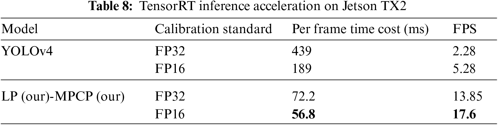
Nowadays, the rapid development of edge computing has driven an increasing number of deep learning applications deployed at the edge of the network, such as pedestrian and vehicle detection, to provide efficient intelligent services to mobile users. However, as the accuracy requirements continue to increase, the components of deep learning models for pedestrian and vehicle detection, such as YOLOv4, become more sophisticated and the computing resources required for model training are increasing dramatically, which in turn leads to significant challenges in achieving effective deployment on resource-constrained edge devices while ensuring the high accuracy performance. For addressing this challenge, a cloud-edge collaboration-based pedestrian and vehicle detection framework is proposed in this paper, which enables sufficient training of models by utilizing the abundant computing resources in the cloud, and then deploying the well-trained models on edge devices, thus reducing the computing resource requirements for model training on edge devices. Furthermore, to reduce the size of the model deployed on edge devices, an automatic pruning method combines the convolution layer and BN layer is proposed to compress the pedestrian and vehicle detection model size. Experimental results show that the framework proposed in this paper is able to deploy the pruned model on a real edge device, Jetson TX2, with 6.72 times higher FPS. Meanwhile, the channel pruning reduces the volume and the number of parameters to 96.77% for the model, and the computing amount is reduced to 81.37%.Keywords
Currently, with the rapid development of deep learning, more and more artificial intelligence applications are beginning to prosper, such as pedestrian and vehicle detection. The maturity of pedestrian and vehicle detection technologies is also driving the development of technologies such as autonomous driving and connected vehicles [1,2]. To achieve better detection performance, pedestrian and vehicle detection implemented based on deep learning models often need to consume a large amount of computing resources for training, which makes high-performance pedestrian and vehicle detection models to be deployed in cloud computing centers with abundant computing resources, far from the end users where the detection demand arises [3]. As a result, when end devices generate detection tasks they need to send the data to the cloud for processing and later return the detection results to the terminal, leading to long delay, which makes it difficult to meet the demand for efficient detection in latency-sensitive applications such as autonomous driving.
Edge computing is a new computing paradigm that greatly reduces the transmission latency of data at the edge by deploying computing resources close to where the data source is generated [4]. By deploying pedestrian and vehicle detection models on edge devices, data such as videos or images generated by surveillance devices are sent to the nearest edge device for processing, greatly improving the efficiency of pedestrian and vehicle detection [5,6]. However, limited by the size of the edge devices, the computing resources deployed by the edge devices are limited and can only enable the training and inference of lightweight deep learning models. The network structure of the model is sophisticated in terms of improving the feature performance of the model to extract video or images, which also makes it difficult for the integrity pedestrian and vehicle detection models to be adequately trained on the edge, resulting in the accuracy of the model is difficult to be guaranteed. At the same time, pedestrian and vehicle detection as a real-time task has a high demand for video and image data performance metrics such as frame per second (FPS). With the increasing number of pedestrians and vehicles, it is difficult for resource-constrained edge devices to ensure detection accuracy while improving detection efficiency. Therefore, deploying pedestrian-vehicle detection models directly on resource-constrained edge devices still faces significant challenges.
To achieve efficient deployment of complex deep learning models, especially pedestrian and vehicle recognition detection models, on resource-constrained edge devices, model compression has received wide attention from academia and industry as a way to reduce the computing and storage resources required for training by reducing the useless parameters of the models, and thus. Currently, model compression can be implemented in four ways, namely quantization [7], low-rank decomposition [8], knowledge distillation [9], and model channel pruning [10]. Among them, quantization [11,12] is used to reduce the memory usage by decreasing the bit width of the parameters and thus achieve the compression of the deep learning model, but special hardware instructions are required to reduce the latency in the process of implementing the model quantization. In addition, low-rank decomposition is used to estimate the parameters of the deep learning model by using tensor decomposition, which in turn achieves the compression of the model. Meanwhile, knowledge distillation is performed by first training a large model with good performance using sufficient computing and labeled data resources, and then knowledge distillation is performed on this model to obtain a small model with a smaller parameter size but comparable performance to the large model, thus achieving the goal of model compression. In addition, the similarities in the structures in the deep learning models make the models have redundant parameters that need to be computed, taking up a large number of computing resources [13]. Model channel pruning removes redundant parameters from a model by implementing sparsity constraints. Specifically, model channel pruning requires initially training a large and over-parameterized model (sometimes pre-trained models can also be used). Subsequently, performing model channel pruning based on model characteristics. Eventually, fine-tuning the pruned model to restore lost accuracy. In general, model channel pruning makes it easier to obtain a compact network that can significantly reduce storage space and computing costs.
However, unreasonable model channel pruning strategies for pedestrian and vehicle detection models based on the important assessment of model channels without considering multiple factors can lead to the loss of important parameters in the model, resulting in a large loss of model accuracy and making the usability of the pruned model impossible to be guaranteed. Meanwhile, the pruning threshold of the model needs to be set empirically, which also makes unreasonable threshold settings lead to a large reduction in the accuracy of pedestrian and vehicle detection models. Furthermore, the pruned deep learning models still need to be fine-tuned, and the complex structure of pedestrian and vehicle detection models makes it difficult to implement effective fine-tuning strategies for pedestrian and vehicle detection models. At the same time, the performance of model channel pruning depends on the sparsity of the model, and sparsity training requires a large number of computing resources, which makes it difficult to implement sparsity training of deep learning models on resource-constrained edge devices.
In this paper, to supplement the computing resource requirements of edge devices for efficient deployment of pedestrian and vehicle detection models at the edge, a cloud-edge collaboration pedestrian and vehicle detection framework is proposed to assist the training of pedestrian and vehicle detection model by leveraging the powerful computing resources deployed in the cloud. In addition, to improve the execution efficiency of trained models on edge devices, an automatic channel pruning method is proposed to achieve compression of trained pedestrian and vehicle detection model to ensure that the computing resources deployed on resource-constrained edge devices can meet the efficient execution demand of the compressed models while ensuring the accuracy of pedestrian and vehicle detection. Meanwhile, to obtain the optimal model channel pruning decision, a new sparsity method for distinguishing model parameters is also proposed.
Specifically, the main contributions of this paper are as following:
• To give full play to the respective advantages of cloud computing and edge computing, a pedestrian and vehicle detection framework based on cloud-edge collaboration is constructed in this paper. Generally, the pedestrian vehicle detection model YOLOv4 is compressed and optimized on the cloud server, and then the compressed lightweight model is delivered to the edge end, and the edge server optimized the speed. Among them, the cloud adopts the optimization method of network pruning, and the edge adopts the optimization method of TensorRT layer and tensor fusion.
• A general deep neural network sparsity method is proposed, which makes the parameter distribution of the model more obvious. It mainly considers the connection between the convolution layer and BN layer, and obtains three influencing factors to determine the model by analyzing the influence of their input on the network output of each layer: BN layer convolution layer weight, BN layer scaling factor and BN layer bias factor, so that corresponding penalty terms are added to these three factors in the loss function to minimize the MAP loss after sparsity training of the model.
• A novel multi-polarization channel-pruning (MPCP) strategy is proposed, which makes the compressed network model smaller in volume, has fewer parameters, less computation and less inference time. It mainly judges the importance of channels by combining the convolution weight, scaling factor and bias factor of the BN layer, and determines the pruning threshold according to the convexity of parameter distribution, to cut out unimportant channels. The experimental results show that the MPCP strategy reduces the number of parameters and volume of the model to 96.77%, the computing amount to 81.37%, and the inference speed of the model by 5.53 times.
The rest of this paper is organized as follows. In Section 2, the related work is listed. Then, a method for optimzation of the pedestrian and vehicle detection model based on cloud-edge collaboration is defined in Section 3. Futhermore, experimental evaluation is presented in Section 4. Finally, conclusion and future work are drawn in Section 5.
Nowadays, with the advent of the era of Internet of Everything, related technologies such as artificial intelligence (AI) and edge computing (EC) have been applied on a wide scale. Meanwhile, the combination of AI and EC is driving the rapid development of edge intelligence [14,15]. As an application that has been widely deployed, target detection, especially pedestrian and vehicle detection, deployed on edge devices can greatly improve the efficiency of target detection while ensuring the privacy of end-users [16,17]. However, as a computation-intensive task, the resources deployed on edge devices make it difficult to ensure that models are adequately trained, which poses a huge challenge for pedestrian and vehicle detection in real-world application scenarios.
To enable the deployment of pedestrian and vehicle detection models on resource-constrained edge devices, lightweight models are developed. Zhang et al. [18] proposed a cross-stage lightweight module that generates redundant features from inexpensive operations and thus reduces the computation overhead. In [19], Xu et al. proposed a lightweight target detection network, which constructs the backbone of the whole model by using G-Module combined with depth-wise convolution, and adds an attention mechanism to weight each channel to obtain more key features and remove redundant features, thus enhancing the detection ability of the feature network model. Meanwhile, some less important channels are removed to compress the size of the model to reduce the computing cost. Wang et al. [20] reconstructed an efficient YOLO framework based on the traditional YOLOv3 by using hierarchical pruning and channel pruning to lighten the parameters of the model. Moreover, an iterative initialization strategy is designed to ensure the sparsity of the network during initial training. In [21], Zhao et al. proposed Mixed YOLOv3-LITE, a lightweight real-time target detection network that can be used for non-graphical processing units (GPUs) and mobile devices, achieving an optimal balance of detection accuracy and speed on non-GPU based computers and portable end devices. Wang et al. [22] pruned the convolution kernel of YOLOv4-tiny and introduced a scalable convolution layer in the residual module of the network, which in turn led to an hourglass cross stage partial ResNet structure, achieving an increase in the mean average accuracy and real-time detection of the model while reducing the model size speed. In addition, the receptive field block simulating human vision are added to increase the receptive field of the model, which in turn enhances the feature extraction capability of the network. Wang et al. [23] proposed a lightweight target detection model based on YOLOv4, which simplifies the network structure and reduces the size of the model parameters, thus enabling further application and development of the target detection model on mobile and embedded devices.
At the same time, channel pruning as a way of model compression to achieve acceleration of deep learning model inference while ensuring that the model has high accuracy [24,25]. Therefore, edge devices can deploy channel-pruned deep learning models to achieve efficient detection of pedestrians and vehicles. In [26], Li et al. proposed a channel pruning method for target detection by using a multi-task sensory loss algorithm to evaluate the contribution of each channel to the final detection, which in turn retains the top-k representative channels and prunes the remaining channels. Chen et al. [27] introduced network building blocks to analyze the YOLOv3-SPP3 and demonstrated the importance of shift factor on channel saliency during pruning. Moreover, a high-ratio channel pruning method is proposed to improve the performance of the pruning model based on the scale factor and shift factor of the batch normalization layer to define the channel saliency. Based on discrimination aware channel pruning, Xie et al. [28] proposed a localization-aware auxiliary network to find out the channels with classification and regression key information, thus directly pruning the channels for target detection and thus reducing a lot of time and computing resources. In [29], Chen et al. proposed a collaborative channel pruning method based on convolutional layer weights and BN layer scaling factors to evaluate the channel importance, which in turn enables the removal of unimportant channels from the model without degrading the model performance. Jin et al. [30] proposed an effective method for dynamically enhancing channel-level sparsity. The channel pruning is achieved by monitoring the saliency of channels to evaluate their importance to the model performance in order to identify the insignificant channels.
To the best of our knowledge, there are few studies on the optimization of the pedestrian and vehicle detection model based on cloud-edge collaboration. Moreover, it is challenging to achieve efficient channel pruning while maintaining the model performance. Therefore, an automatic pruning method combining convolutional and BN layers is proposed in this paper to compress the model size and thus achieve efficient pedestrian and vehicle detection in cloud-edge collaborative scenarios.
To achieve efficient deployment of pedestrian and vehicle detection models at the edge, a pedestrian and vehicle detection framework based on cloud-edge collaboration is proposed in this paper, as shown in Fig. 1. Specifically, initially, a YOLOv4-based pedestrian and vehicle detection model is constructed, and the pedestrian and vehicle detection model is trained until the model accuracy is optimal by using the abundant computing resources deployed in the cloud and the huge amount of historical data. Then, the pedestrian and vehicle detection model is compressed by the model channel pruning strategy to reduce the number of parameters and scale of the models as possible without excessive loss of accuracy. Finally, the compressed pedestrian and vehicle detection model is deployed on the edge devices, which enables the inference of pedestrian and vehicle detection models to be implemented close to the location where the data sources are generated, ensuring that pedestrian and vehicle detection applications can be efficiently executed on the resource-constrained edge devices. Meanwhile, the historical data collected at the edge devices will be sent to the cloud periodically to enable scheduled updates of the pedestrian and vehicle detection model.
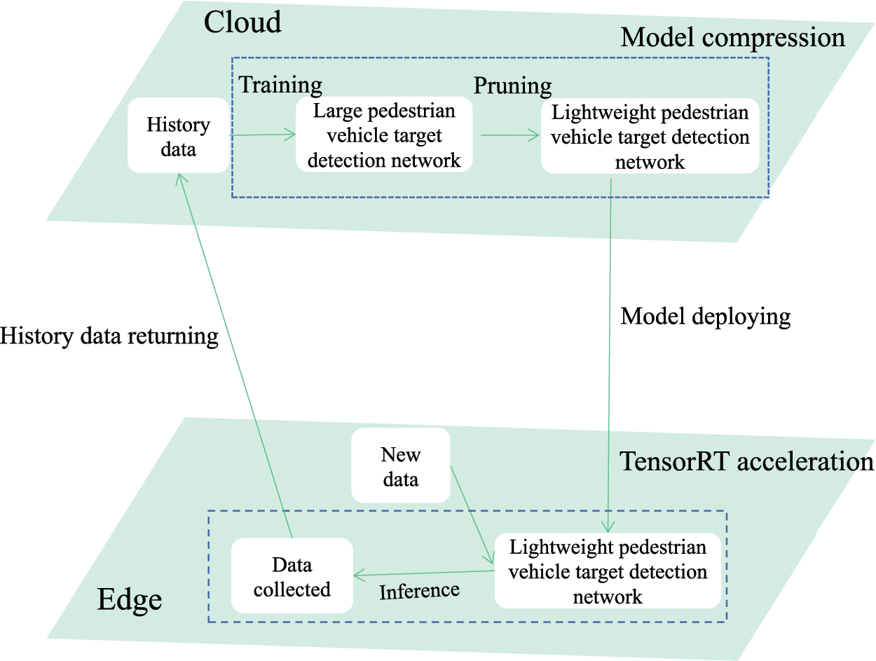
Figure 1: A framework of pedestrian and vehicle detection based on cloud-edge collaboration
Meanwhile, the workflow of the proposed framework in this paper is shown in Fig. 2. In particular, images of pedestrians and vehicles are collected by the cameras deployed on the roadside and sent to the cloud data center, and pre-processing of the images of pedestrians and vehicles is implemented in the cloud. Then, the sufficient computing resources deployed in the cloud are leveraged to train the pedestrian and vehicle detection model based on YOLOv4. Subsequently, sparsity training is performed on the parameters (YOLOv4.weight) of the trained models to obtain the sparsity model parameters (YOLOv4.pt). Furthermore, channel pruning is conducted on the pedestrian and vehicle detection model to obtain the compressed model parameters (SilmYOLOv4.weight). Finally, the compressed pedestrian and vehicle detection model is deployed on the edge devices to implement the inference of the pedestrian and vehicle detection models. Moreover, TensorRT is used to accelerate the inference of the models during the inference of pedestrian and vehicle detection on edge devices. In addition, latency-sensitive and non-latency-sensitive pedestrian and vehicle detection tasks are considered in this paper. 1) When the detection task comes from a latency-sensitive application, the task is sent to the edge device to achieve pedestrian and vehicle recognition by utilizing the deployed compressed pedestrian and vehicle detection models, which in turn reduces the data transmission latency. 2) When the detection task comes from a non-latency-sensitive application, the task-related data is sent to the cloud for pedestrian and vehicle detection, relieving the computing and network pressure of the edge devices.
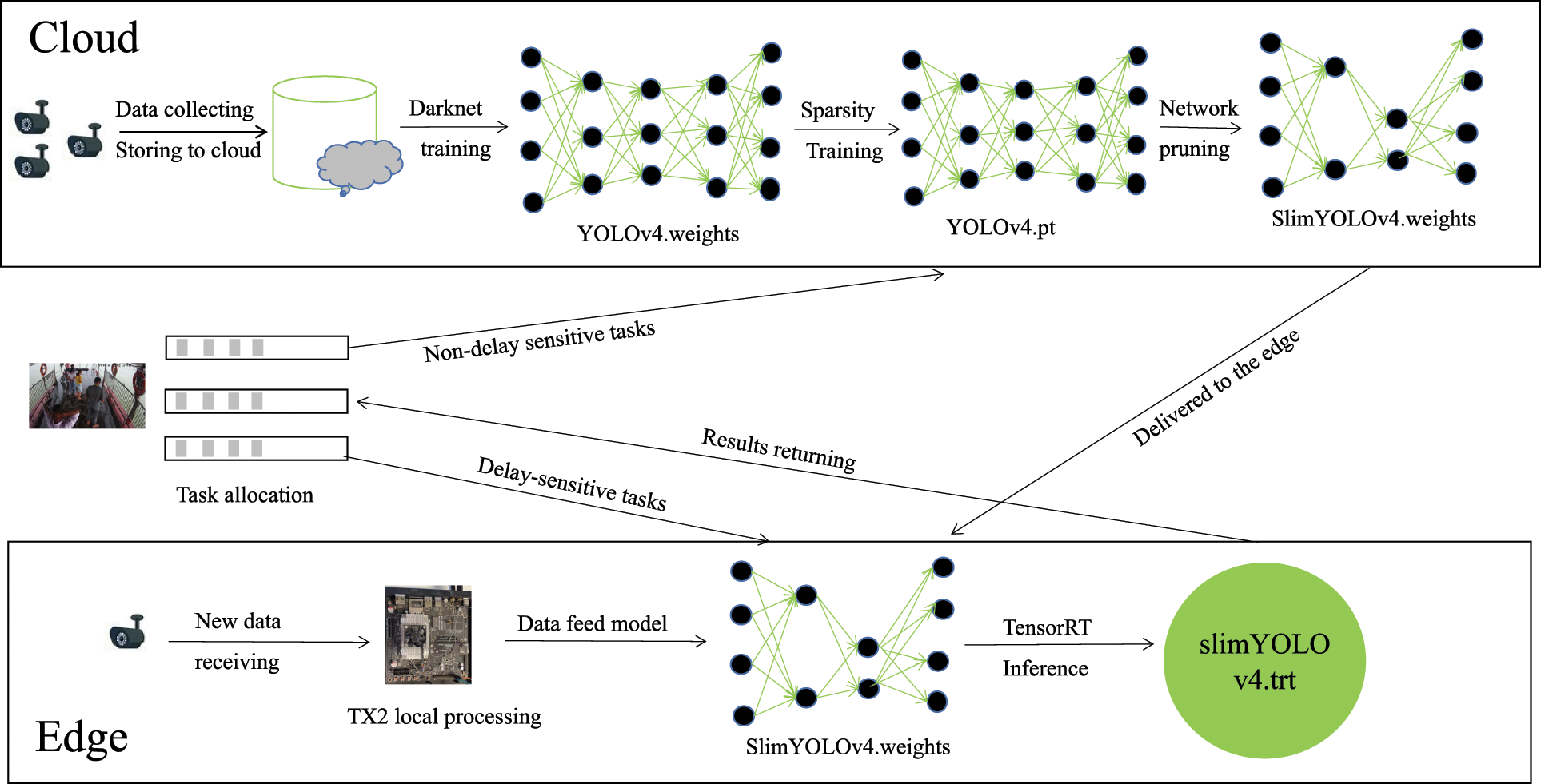
Figure 2: The workflow of cloud-edge collaboration pedestrian and vehicle detection framework
3.2 Correlation Factor Analysis
To implement channel pruning for pedestrian and vehicle detection models, the structure of YOLOv4 is analyzed in depth in this paper. YOLOv4 is an improved version of YOLOv3, and its core structure is similar to YOLOv3, but the performance of target detection is further improved by incorporating several new network structures. the structure of YOLOv4 network can be divided into three parts: Backbone, Neck and Head. The backbone network is based on the CSPNet structure and incorporates DarkNet53 [31], which makes the performance of the backbone network significantly improved. Besides, the Neck of YOLOv4 is mainly composed of SPP [32] and PAN [33]. The output feature layer of the backbone network is processed to widen the receptive field, enhance the extraction of feature maps, and effectively prevent overfitting. Furthermore, the Head of YOLOv4 is the same as YOLOv3, which still uses a three-scale output for the detection of targets with different sizes, and the heads with sizes 1/8, 1/16, and 1/32 of the original input size are used for the detection of large, medium, and small targets, respectively [34].
Based on the above analysis, the convolutional layer plays an important role in YOLOv4. To achieve efficient channel pruning, the inputs and outputs of the convolutional layer of the model need to be analyzed. the convolutional operation in YOLOv4 is represented by Eq. (1).
where
When BN layer is not added to standardize the input value, it can be seen from Eq. (1) that the output of the first layer is determined by
The function of batch BN layer [36] is to standardize input values and reduce numerical differences to the same range. On the one hand, the convergence degree of gradient is improved and the training speed of the model is accelerated. On the other hand, each layer can face the input value of the same feature distribution as far as possible, which reduces the uncertainty brought by the change and also reduces the influence on the subsequent network layer. The network of each layer becomes relatively independent, which alleviates the problem of gradient disappearance in training. The BN layer first calculates the expectation and variance of its input, as shown in Eqs. (3) and (4).
where M is the batch size that represents the input to the BN layer of the first layer. Then, the BN layer normalizes its input by the expected value and variance, and the transformation of the BN layer can be represented by Eq. (5).
where
According to Eq. (6), the output of the
3.3 LP Sparsity Regularization
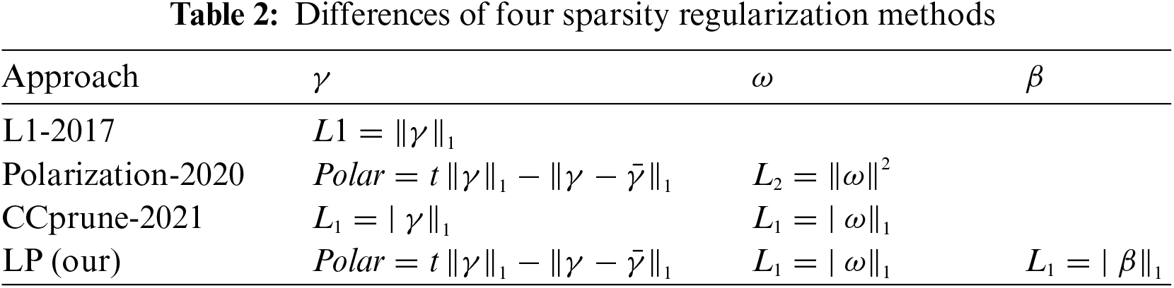
After correlation factor analysis in Section 3.2, it can be concluded that the output of the model is not only related to BN layer, but also related to convolution layer. Zhuang et al. [37] also carried out different punishment treatments for the parameters of the two layers, proposed their own regularization method for the parameters of BN layer, and used L2 regularization for the weights of the convolution layer. However, we believe that L2 regularization of network weights is of little significance. It is well known that L2 regularization penalizes large numerical weights and encourages smaller values. However, a small parameter does not mean that the parameter is 0. L1 sparsity will generate many values of 0, and then the weight of 0 will be cut off, which will have no impact on the model. Chen et al. [29] used L1 regularization for both
Therefore, the training loss function of the pedestrian and vehicle detection model is defined in this paper as follows:
where
The most important thing for channel pruning is to find a reasonable method to evaluate the importance, then determine the appropriate threshold value, and then cut off the non-important channels or layers according to the threshold value to minimize the loss. In Section 3.2, the network structure for YOLOv4 is analyzed and concluded that the BN layer output is related to three learnable parameters
The process of the MPCP is shown in Fig. 3. From left to right, the first three-dimensional graph represents the input characteristic graph of the
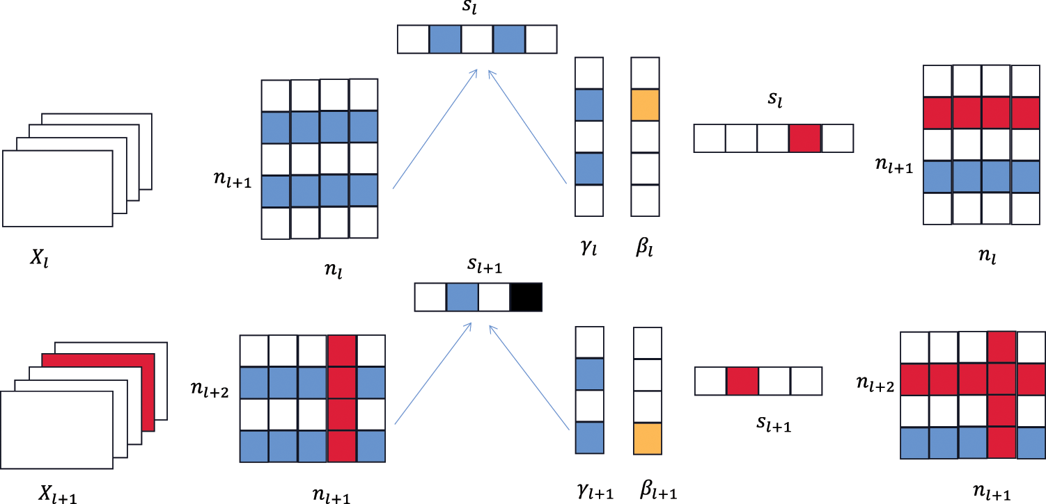
Figure 3: The pruning process of the MPCP
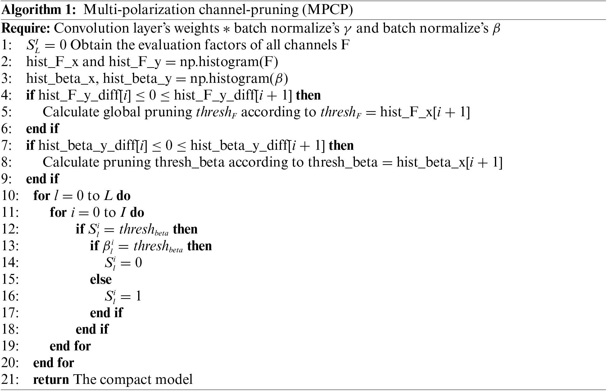
Algorithm 1 firstly obtains the evaluation factors of all channels according to formula
3.5 Acceleration of Edge Inference
When pruned pedestrian and vehicle and detection models are deployed to the edge devices, new real-time image data is sent to the edge devices and the pruned models are used for inference to achieve pedestrian and vehicle detection, which greatly reduces the data transmission latency. However, when the number of pedestrian and vehicle detection tasks increases drastically, the computing resources deployed in the edge devices have difficulty in meeting the response speed of delay-sensitive pedestrian and vehicle detection inference tasks. Therefore, the TensorRT layer and tensor fusion are leveraged in the proposed framework to optimize the inference speed of the model, and the semi-floating point precision quantization method is also used to reduce the memory occupation of the model for better pedestrian and vehicle detection. The flowchart of edge inference acceleration is shown in Fig. 4.
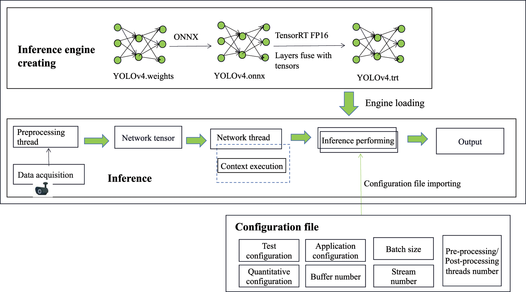
Figure 4: The flow chart of edge inference acceleration
The configuration file needs to be loaded first and multiple threads are used to do edge inference. The configuration file is determined by the parameters to be optimized. When the onboard camera of Jetson TX2 captures new images, these images need to be pre-processed and converted into the tensor needed for the model input. Moreover, a network thread needs to take the pruned lightweight model to be transformed into an inference engine that TensorRT can accelerate, and another network thread adopts the input data to execute the context. The inference engine is then loaded, the configuration file is imported to accelerate the model, and the inference results are output.
In this paper, a server with Intel Xeon E5-2678 v3 @2.50 GHz, 32 GB RAM, NVIDIA GTX2080Ti GPU and Ubuntu 18.04.5LTS is utilized as the cloud server. Meanwhile, the Jetson Tegra X2 with a six-core CPU, Pascal GPU and with 8GB of global memory is utilized as the edge device.
4.2 Dataset and Evaluation Indexes
The dataset used in this experiment is pedestrian-vehicle data collected from a commercial company, containing 3008 images taken by surveillance cameras at different time periods, which is not publicly available. In addition, the dataset consists of 2402 images as the training set and 606 images as the validation set. These images are manually labeled into four predefined categories (i.e., people, heads, motorcycles, and bicycles).
Meanwhile, to validate the performance of the model, the evaluation metrics used in the experiments are (1) MAP, (2) Parameters, (3) Volume, (4) FLOPs, (5) Inference time, and (6) FPS. In generally, FPS is the transmission frame rate per second, which represents how many images per second the target network can detect. The effectiveness of the MPCP strategy is verified using the inference time, and the effectiveness of the model compression method is verified using the FPS.
The YOLOv4 [34] is chosen as the benchmark network for this experiment, and the Darknet is utilized for training to get various indicators of pedestrian vehicle detection network, as shown in Fig. 5.
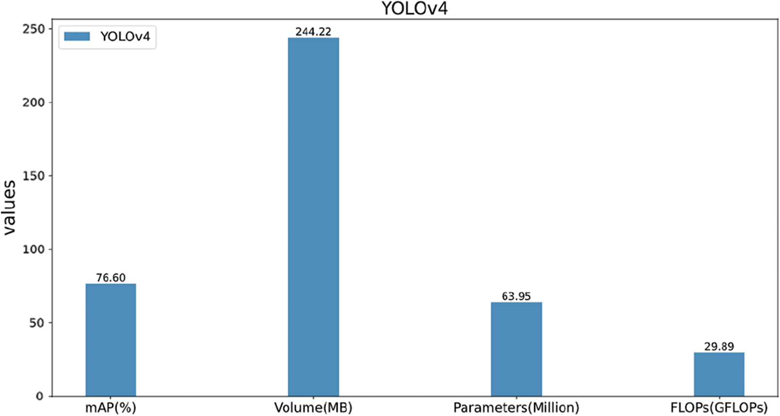
Figure 5: YOLOv4 model indicators
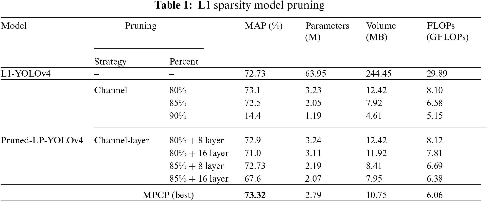
Subsequently, L1 regularization proposed by Liu et al. [38] are used for sparse training of YOLOv4, and channel pruning and channel-layer pruning are carried out, and the pruned model is used as the basic model for comparison. The experimental results are shown in Table 1.
4.4 Comparison of Different Sparsity Training
4.4.1 Differences between Sparsity Regularization
As shown in Table 2, the benchmark method of the experiment is L1 [38], which only performs L1 regularization for
4.4.2 Verify the Effectiveness of Sparsity Regularization of
In this subsection, the influence of sparsity on
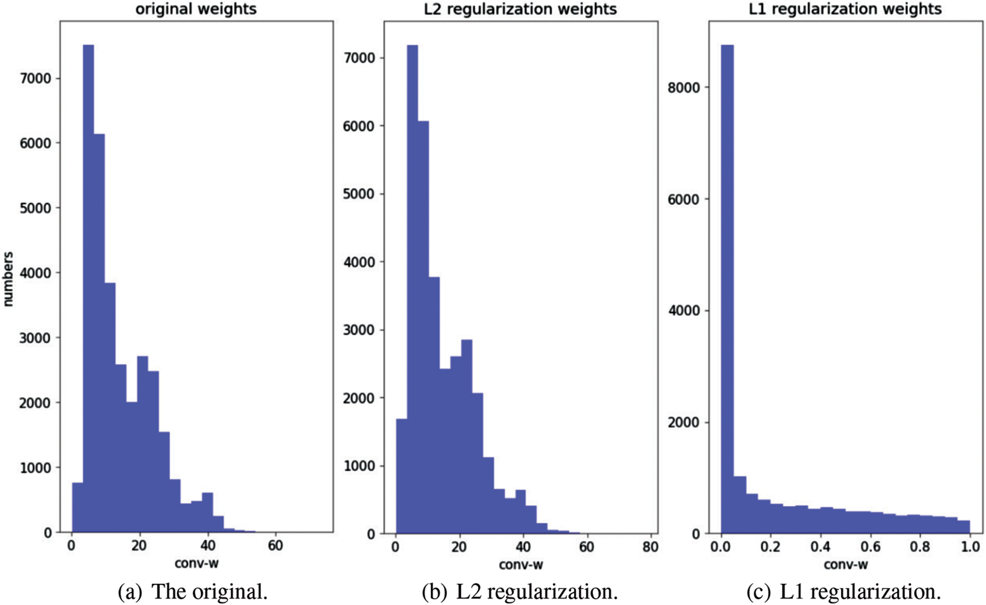
Figure 6: The satistical histogram of
Furthermore, the effect of regularization on
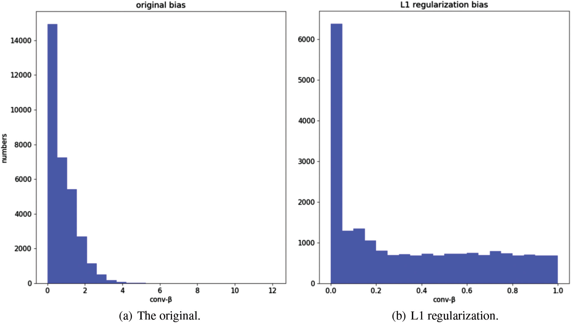
Figure 7: The statistical histogram of
4.4.3 Verify the Effectiveness of Sparsity Regularization on MAP
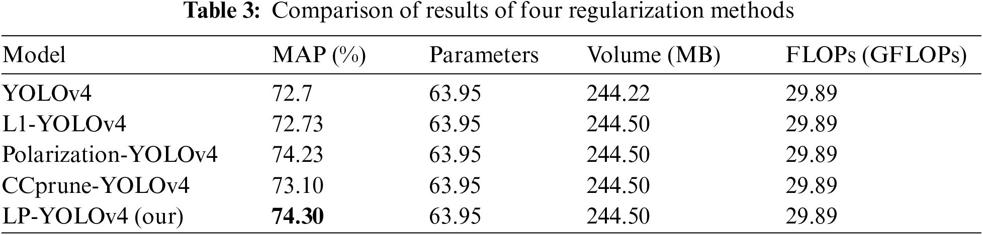
As shown in Table 3, compared with the non-sparse YOLOv4, the metrics such as the number of model parameters, volume size and FLOPs remain the same after different sparsity methods, but there is a certain improvement in MAP. Among them, The MAP after L1 sparsity and CCPrune sparsity are 72.73% and 73.10%, respectively. However, the MAP of the polarization sparsity and the LP sparsity are 74.23% and 74.30%, respectively, which demonstrates the effectiveness of the polarization sparsity and the LP sparsity. Meanwhile, the accuracy of the LP sparsity is higher compared to the polarization sparsity, which also demonstrates the effectiveness of the LP sparsity.
4.5 Comparison of Different Pruning
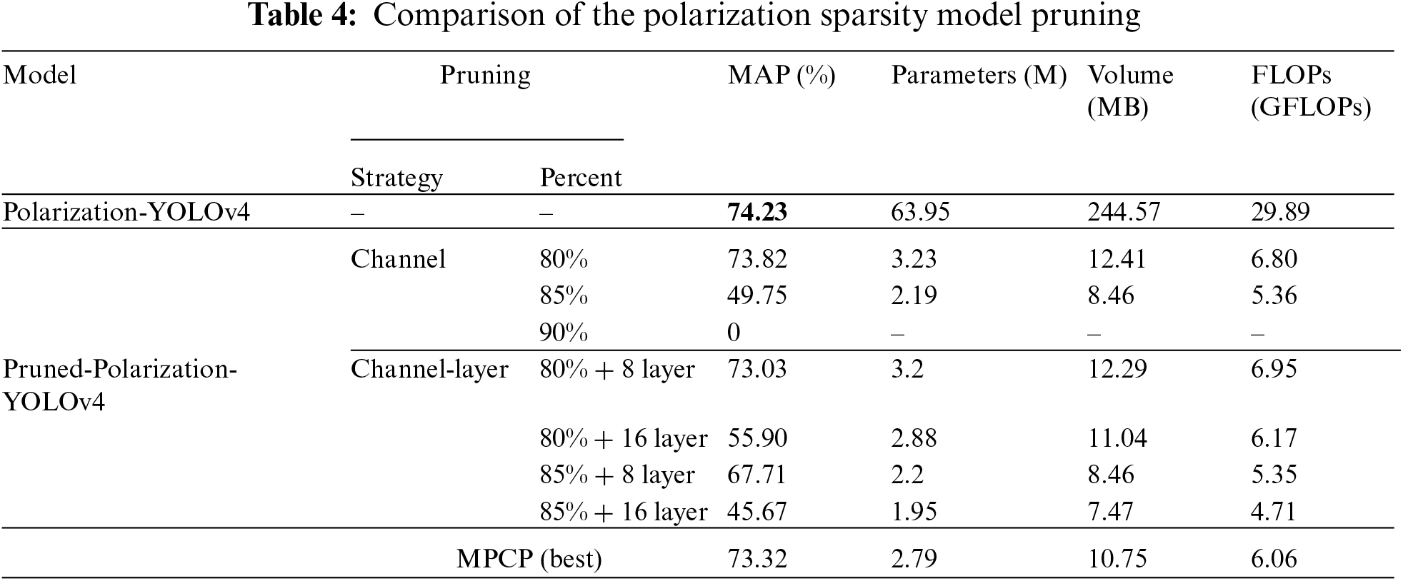
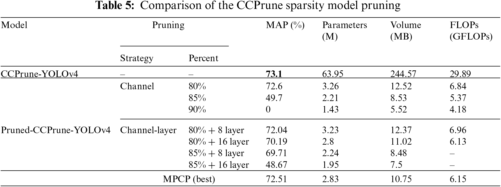
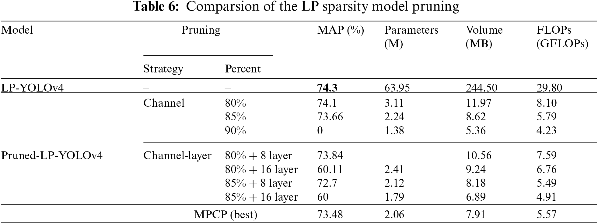
To verify the effectiveness of MPCP, three sparsity models with channel pruning and channel-layer pruning are leveraged for comparative experiments. The results with different sparsity models are shown in Tables 4–6, respectively. In general, compared with Polarization-YOLOv4 and CCPrune-YOLOv4, LP-YOLOv4 is the best in terms of MAP performance with little difference in the number of parameters, volume and FLOPs values. Meanwhile, under the three different models, the number of model parameters and volume keep decreasing by increasing the ratio of channel pruning, but the MAP performance also shows a sharp decline, which can even lead to the model not working at all. However, MPCP achieves the premise that the model parameters and volume are drastically reduced under the three models, and still ensures that the model has a high MAP performance, which fully demonstrates the effectiveness of MPCP.
4.5.2 Verify the Effectiveness of Sparsity Method on Pruning
The comparison of the effectiveness of pruning under different sparsity methods is shown in Fig. 8. In Fig. 8a, the MAP performance of channel pruning with different pruning rates is shown, and it can be seen that when the pruning rate of the channel is set to 80%, the MAP performance of the LP sparsity method is the best. And when the channel pruning rate is set to 85%, the MAP performance of the polarization sparsity and the CCPrune sparsity decreases more significantly to about 50%, while the MAP of the LP sparsity and L1 sparsity does not decrease significantly. Meanwhile, the MAP performance of the LP sparsity decreases less than that of the L1 sparsity, which in turn indicates that the LP sparsity has the best performance. Furthermore, when the channel pruning rate is set to 90%, the accuracy of the polarization sparsity, the CCPrune sparsity and the LP sparsity loses almost all, and the accuracy of the L1 sparsity also decreases significantly, which also indicates that the model is useless when the pruning rate is too high.
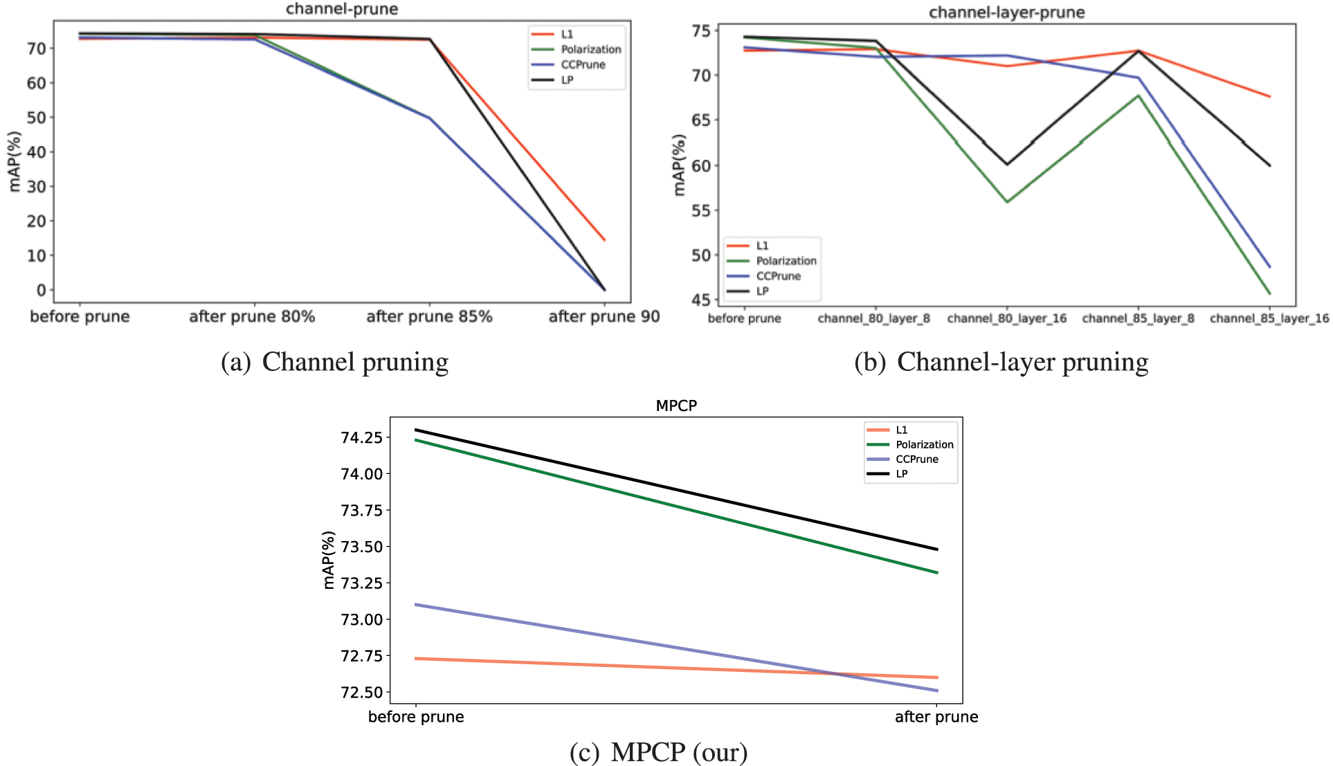
Figure 8: Comprasion of the effectiveness with different sparsity method on pruning
As shown in Fig. 8b, the MAP performance of the pedestrian and vehicle detection model after channel-layer pruning at different pruning rates. It can be seen that when the pruning rate is set to 80% and the number of channels removed layers is set to 8, the MAP performance of the model after the four methods of sparsity does not show an excessive loss, but the MAP performance of the model after LP sparsity is optimal. And when the pruning rate is set to 80% and the number of channel removed layers is set to 16, the MAP performance of CCPrune is the best. Moreover, when the pruning rate is set to 85% and the number of channels removed is set to 8, the MAP performance of the model processed by the L1 sparsity and the LP sparsity is the same. Furthermore, when the pruning rate is set to 85% and the number of channels removed layers is 16, the MAP performance of the model processed by the L1 sparsity is optimal, and LP sparsity is sub-optimal, while the MAP performance of the model processed by the polarization and CCPrune sparsity is too high in terms of performance loss.
The performance of MAP under the MPCP strategy is shown in Fig. 8c. The pruning needs to be executed just once under the MPCP strategy without multiple trials. After pruning is completed, the LP sparsity performs the best MAP performance and the CCPrune sparsity has the lowest MAP performance. In addition, the MAP performance of the polarization sparsity decreases more significantly. Therefore, the LP sparsity method has the best MAP performance under the MPCP strategy.
4.5.3 Verify the Effectiveness of Pruning Strategy on FPS
In this subsection, to verify the performance of the proposed sparsity method LP and pruning strategy MPCP on model inference time, we conduct experiments on the model performance after LP and MPCP processing. As shown in Fig. 9, the performance of the model is in terms of the number of parameters, FLOPs and inference time after channel pruning, channel layer pruning and MPCP pruning. Specifically, compared with channel pruning and channel-layer pruning, MPCP can significantly reduce the number of parameters and increase the inference speed of the model without losing too much accuracy, further demonstrating the effectiveness of the proposed method.
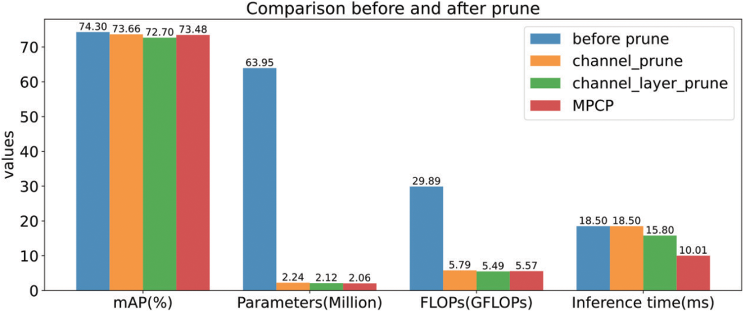
Figure 9: Comparison of three pruning methods
4.6 Comparing Edge Deployment Results
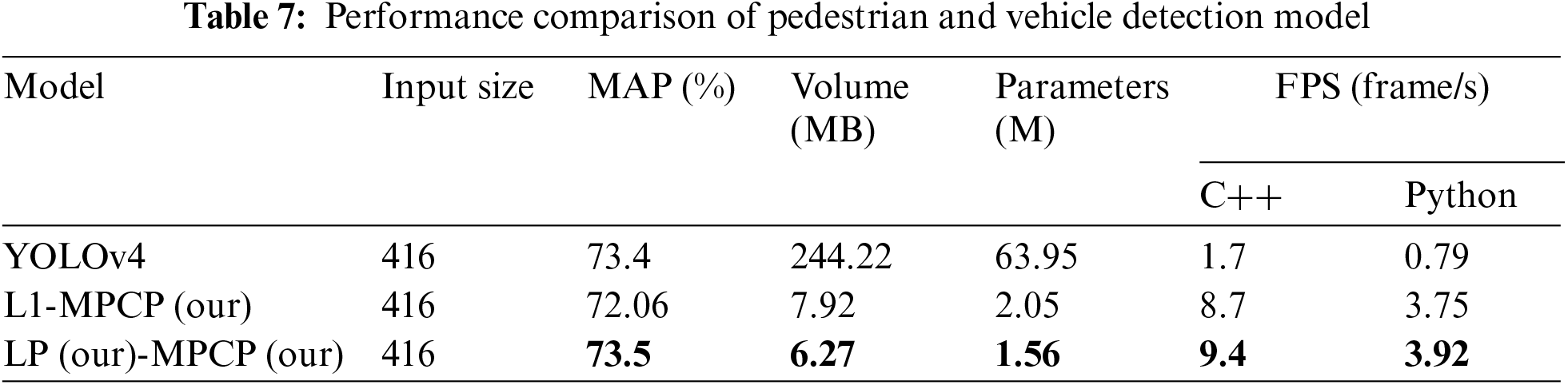
As shown in Table 7, compared with the original YOLOv4, the pruned model is faster and more accurate. When the model input image is 416
In this paper, a pedestrian and vehicle detection framework based on cloud-edge collaboration is proposed to achieve efficient deployment of the pedestrian and vehicle detection model on edge devices. Specifically, initially, the pedestrian and vehicle detection models built on yolov4 are trained by utilizing sufficient computing resources deployed in the cloud computing center. Then, the model is compressed using model channel pruning techniques, and the compressed model is deployed on edge devices to reduce the resource overhead required for model training. Finally, TensorRT layer and tensor fusion optimization methods are used on the edge devices to further improve the accuracy of the model. In addition, a general DNN sparsity method is proposed to achieve a more distinct parameter distribution of the model, which in turn improves the MAP performance of the model. Furthermore, a new multi-polarization channel pruning strategy, MPCP, is proposed in this paper making the compressed model smaller in size and with fewer parameters while ensuring no excessive loss of accuracy. Numerous experimental results demonstrate the effectiveness of the method proposed in this paper.
Regarding future work, we will make further improvements to deploy the method proposed in this paper in the actual cloud-edge collaboration scenario for implementing efficient pedestrian and vehicle detection. Moreover, we will consider incorporating efficient data pre-processing techniques into the edge training process to further the efficiency and accuracy of model training and inference on edge devices.
Acknowledgement: We are grateful to the editors and reviewers for their helpful suggestions, which have greatly improved this paper.
Funding Statement: This work is supported by Key-Area Research and Development Program of Guangdong Province (2021B0101420002), the Major Key Project of PCL (PCL2021A09), National Natural Science Foundation of China (62072187), Guangdong Major Project of Basic and Applied Basic Research (2019B030302002), Guangdong Marine Economic Development Special Fund Project (GDNRC[2022]17) and Guangzhou Development Zone Science and Technology (2021GH10, 2020GH10).
Conflicts of Interest: The authors declare that they have no conflicts of interest to report regarding the present study.
References
1. Boukerche, A., Sha, M. (2021). Design guidelines on deep learning–based pedestrian detection methods for supporting autonomous vehicles. ACM Computing Surveys (CSUR), 54(6), 1–36. [Google Scholar]
2. Camara, F., Bellotto, N., Cosar, S., Weber, F., Nathanael, D. et al. (2020). Pedestrian models for autonomous driving Part II: High-level models of human behavior. IEEE Transactions on Intelligent Transportation Systems, 22(9), 5453–5472. https://doi.org/10.1109/TITS.2020.3006767 [Google Scholar] [CrossRef]
3. Rasouli, A., Tsotsos, J. K. (2019). Autonomous vehicles that interact with pedestrians: A survey of theory and practice. IEEE Transactions on Intelligent Transportation Systems, 21(3), 900–918. https://doi.org/10.1109/TITS.2019.2901817 [Google Scholar] [CrossRef]
4. Premsankar, G., di Francesco, M., Taleb, T. (2018). Edge computing for the Internet of Things: A case study. IEEE Internet of Things Journal, 5(2), 1275–1284. https://doi.org/10.1109/JIOT.2018.2805263 [Google Scholar] [CrossRef]
5. Liu, S., Liu, L., Tang, J., Yu, B., Wang, Y. et al. (2019). Edge computing for autonomous driving: Opportunities and challenges. Proceedings of the IEEE, 107(8), 1697–1716. https://doi.org/10.1109/JPROC.2019.2915983 [Google Scholar] [CrossRef]
6. Su, C. L., Lai, W. C., Li, C. T. (2021). Pedestrian detection system with edge computing integration on embedded vehicle. 2021 International Conference on Artificial Intelligence in Information and Communication (ICAIIC), pp. 450–453. Jeju Island, Korea (South). https://doi.org/10.1109/ICAIIC51459.2021.9415262 [Google Scholar] [CrossRef]
7. Kryzhanovskiy, V., Balitskiy, G., Kozyrskiy, N., Zuruev, A. (2021). Qpp: Real-time quantization parameter prediction for deep neural networks. Proceedings of the IEEE/CVF Conference on Computer Vision and Pattern Recognition (CVPR), pp. 10684–10692. Virtual Event. [Google Scholar]
8. Xu, Y., Li, Y., Zhang, S., Wen, W., Wang, B. et al. (2020). Trp: Trained rank pruning for efficient deep neural networks. arXiv preprint arXiv:2004.14566. [Google Scholar]
9. Liu, Y., Shu, C., Wang, J., Shen, C. (2020). Structured knowledge distillation for dense prediction. IEEE Transactions on Pattern Analysis and Machine Intelligence, 1. https://doi.org/10.1109/TPAMI.2020.3001940 [Google Scholar] [PubMed] [CrossRef]
10. Blalock, D., Gonzalez Ortiz, J. J., Frankle, J., Guttag, J. (2020). What is the state of neural network pruning? Proceedings of Machine Learning and Systems, 2, 129–146. [Google Scholar]
11. Zhao, K., Huang, S., Pan, P., Li, Y., Zhang, Y. et al. (2021). Distribution adaptive INT8 quantization for training CNNs. Proceedings of the AAAI Conference on Artificial Intelligence, 35(4), 3483–3491. https://doi.org/10.1609/aaai.v35i4.16462 [Google Scholar] [CrossRef]
12. He, Y., Liu, P., Wang, Z., Hu, Z., Yang, Y. (2019). Filter pruning via geometric median for deep convolutional neural networks acceleration. Proceedings of the IEEE/CVF Conference on Computer Vision and Pattern Recognition (CVPR), pp. 4340–4349. Long Beach, CA. [Google Scholar]
13. Wang, H., Qin, C., Zhang, Y., Fu, Y. (2021). Emerging paradigms of neural network pruning. arXiv preprint arXiv:2103.06460. [Google Scholar]
14. Zhou, Z., Chen, X., Li, E., Zeng, L., Luo, K. et al. (2019). Edge intelligence: Paving the last mile of artificial intelligence with edge computing. Proceedings of the IEEE, 107(8), 1738–1762. https://doi.org/10.1109/JPROC.2019.2918951 [Google Scholar] [CrossRef]
15. Zhang, J., Letaief, K. B. (2019). Mobile edge intelligence and computing for the internet of vehicles. Proceedings of the IEEE, 108(2), 246–261. https://doi.org/10.1109/JPROC.2019.2947490 [Google Scholar] [CrossRef]
16. Chen, J., Ran, X. (2019). Deep learning with edge computing: A review. Proceedings of the IEEE, 107(8), 1655–1674. https://doi.org/10.1109/JPROC.2019.2921977 [Google Scholar] [CrossRef]
17. Ren, J., Guo, Y., Zhang, D., Liu, Q., Zhang, Y. (2018). Distributed and efficient object detection in edge computing: Challenges and solutions. IEEE Network, 32(6), 137–143. https://doi.org/10.1109/MNET.2018.1700415 [Google Scholar] [CrossRef]
18. Zhang, Y. M., Lee, C. C., Hsieh, J. W., Fan, K. C. (2021). Csl-yolo: A new lightweight object detection system for edge computing. arXiv preprint arXiv:2107.04829. [Google Scholar]
19. Xu, H., Guo, M., Nedjah, N., Zhang, J., Li, P. (2022). Vehicle and pedestrian detection algorithm based on lightweight YOLOv3-promote and semi-precision acceleration. IEEE Transactions on Intelligent Transportation Systems, 23(10), 19760–19771. https://doi.org/10.1109/TITS.2021.3137253 [Google Scholar] [CrossRef]
20. Wang, Z., Zhang, J., Zhao, Z., Su, F. (2020). Efficient YOLO: A lightweight model for embedded deep learning object detection. 2020 IEEE International Conference on Multimedia & Expo Workshops (ICMEW), pp. 1–6. London, UK. https://doi.org/10.1109/ICMEW46912.2020.9105997 [Google Scholar] [CrossRef]
21. Zhao, H., Zhou, Y., Zhang, L., Peng, Y., Hu, X. et al. (2020). Mixed YOLOv3-lite: A lightweight real-time object detection method. Sensors, 20(7), 1861. https://doi.org/10.3390/s20071861 [Google Scholar] [PubMed] [CrossRef]
22. Wang, G., Ding, H., Yang, Z., Li, B., Wang, Y. et al. (2022). TRC-YOLO: A real-time detection method for lightweight targets based on mobile devices. IET Computer Vision, 16(2), 126–142. https://doi.org/10.1049/cvi2.12072 [Google Scholar] [CrossRef]
23. Wang, C., Tong, X., Gao, R., Yan, L. (2022). Mobile-YOLO: A lightweight and efficient implementation of object detector based on yolov4. In: Hu, Z., Dychka, I., Petoukhov, S., He, M. (Eds.Advances in computer science for engineering and education, pp. 221–234. Springer, Cham. https://doi.org/10.1007/978-3-031-04812-8_19 [Google Scholar] [CrossRef]
24. Deng, L., Li, G., Han, S., Shi, L., Xie, Y. (2020). Model compression and hardware acceleration for neural networks: A comprehensive survey. Proceedings of the IEEE, 108(4), 485–532. https://doi.org/10.1109/JPROC.2020.2976475 [Google Scholar] [CrossRef]
25. Mishra, R., Gupta, H. P., Dutta, T. (2020). A survey on deep neural network compression: Challenges, overview, and solutions. arXiv preprint arXiv:2010.03954. [Google Scholar]
26. Li, S., Xue, L., Feng, L., Wang, Y. F., Wang, D. (2022). Object detection network pruning with multi-task information fusion. World Wide Web, 25, 1667–1683. https://doi.org/10.1007/s11280-021-00991-3 [Google Scholar] [CrossRef]
27. Chen, Y., Li, R., Li, R. (2021). HRCP: High-ratio channel pruning for real-time object detection on resource-limited platform. Neurocomputing, 463, 155–167. https://doi.org/10.1016/j.neucom.2021.08.046 [Google Scholar] [CrossRef]
28. Xie, Z., Zhu, L., Zhao, L., Tao, B., Liu, L. et al. (2020). Localization-aware channel pruning for object detection. Neurocomputing, 403(3), 400–408. https://doi.org/10.1016/j.neucom.2020.03.056 [Google Scholar] [CrossRef]
29. Chen, Y., Wen, X., Zhang, Y., Shi, W. (2021). CCPrune: Collaborative channel pruning for learning compact convolutional networks. Neurocomputing, 451, 35–45. https://doi.org/10.1016/j.neucom.2021.04.063 [Google Scholar] [CrossRef]
30. Jin, Y., Liu, T., Chen, J., Fu, Y. (2021). Dynamic channel pruning for real-time object detection networks. International Conference on Neural Information Processing, Springer International Publishing, Sanur, Bali, Indonesia. [Google Scholar]
31. Wang, C. Y., Liao, H. Y. M., Wu, Y. H., Chen, P. Y., Hsieh, J. W. et al. (2020). CSPNet: A new backbone that can enhance learning capability of CNN. Proceedings of the IEEE/CVF Conference on Computer Vision and Pattern Recognition (CVPR) Workshops, pp. 390–391. Virtual Event. [Google Scholar]
32. He, K., Zhang, X., Ren, S., Sun, J. (2015). Spatial pyramid pooling in deep convolutional networks for visual recognition. IEEE Transactions on Pattern Analysis and Machine Intelligence, 37(9), 1904–1916. https://doi.org/10.1109/TPAMI.2015.2389824 [Google Scholar] [PubMed] [CrossRef]
33. Liu, S., Qi, L., Qin, H., Shi, J., Jia, J. (2018). Path aggregation network for instance segmentation. Proceedings of the IEEE Conference on Computer Vision and Pattern Recognition (CVPR), pp. 8759–8768. Salt Lake City, Utah. [Google Scholar]
34. Bochkovskiy, A., Wang, C. Y., Liao, H. Y. M. (2020). YOLOv4: Optimal speed and accuracy of object detection. arXiv preprint arXiv:2004.10934. [Google Scholar]
35. Li, H., Kadav, A., Durdanovic, I., Samet, H., Graf, H. P. (2016). Pruning filters for efficient convnets. arXiv preprint arXiv:1608.08710. [Google Scholar]
36. Santurkar, S., Tsipras, D., Ilyas, A., Madry, A. (2018). How does batch normalization help optimization? Advances in Neural Information Processing Systems, 31, 1–11. [Google Scholar]
37. Zhuang, T., Zhang, Z., Huang, Y., Zeng, X., Shuang, K. et al. (2020). Neuron-level structured pruning using polarization regularizer. Advances in Neural Information Processing Systems, 33, 9865–9877. [Google Scholar]
38. Liu, Z., Li, J., Shen, Z., Huang, G., Yan, S. et al. (2017). Learning efficient convolutional networks through network slimming. Proceedings of the IEEE International Conference on Computer Vision (ICCV), pp. 2736–2744. Venice, Italy. [Google Scholar]
Cite This Article
 Copyright © 2023 The Author(s). Published by Tech Science Press.
This work is licensed under a Creative Commons Attribution 4.0 International License , which permits unrestricted use, distribution, and reproduction in any medium, provided the original work is properly cited.
 Downloads
 Citation Tools