Parameterization Transfer for a Planar Computational Domain in Isogeometric Analysis

1  Introduction

In computer-aided design (CAD), boundary representation is one of the main methods for representing three-dimensional (3D) shapes. The process of obtaining a solid spline representation of a computational domain from a given boundary is called parameterization. For planar geometries, parameterization means finding a B-spline surface representation from given boundary curves. The quality of the parameterization of the computational domain has a great impact on the computational accuracy and efficiency in isogeometric analysis (IGA), which is similar to the influence of the mesh quality in finite element analysis. Usually, the parameterization of a computational domain suitable for IGA satisfies the following three basic requirements: (1) Regularization. The mapping from the parametric domain to the physical domain should be injective. Therefore, there is no self-intersection in the iso-parametric structures. (2) Uniformity. The iso-parametric lines are as uniform as possible. (3) Orthogonality. Orthogonality of the iso-parametric structures is preferred in IGA.

In this paper, we propose a parameterization transfer algorithm from one planar domain to another domain, where the two domains have similar shapes, and the parameterization of one domain is given. The geometry with a given parameterization is called the source model, and the other is called the target model. The parameterization of the target model with the transfer algorithm is C1/G1 continuous regardless of whether the source model is C1/G1 continuous or not. The boundaries of the two planar domains are B-spline curves. Therefore, boundary control points of the two planar domains need to be matched first, and the parameterization transfer process is to map the internal control points of the source model to the interior of the target model. The parameterization transfer we proposed meets the following three requirements: (1) Injectivity. The resulting parameterization does not have self-intersection. (2) Low distortion. As the two planar domains are similar in our algorithm, if the parameterization of the source model has high quality, the resulting parameterization also has high quality if the distortion of the map is as small as possible. (3) C1/G1 continuity. Whether the parameterization of the source model satisfies C1/G1 continuity or not, we hope the resulting parameterization has this continuity without additional post-processing.

We use the method proposed by Xu et al. [1] to parameterize the source model. The parameterization transfer process roughly consists of the following two steps:

•   Construct boundary correspondence. First, we extract the boundary splines of the source model in the counter-clockwise direction, and then we process the boundary of the target model to obtain a boundary representation that is also in the counter-clockwise direction. Second, the number of control points on the boundaries of the target model ns may not be the same as that of the source model nt. If nt>ns, we will re-parameterize the boundary of the target model to make  nt=ns. Otherwise, refinement will be performed on the target model to make  nt=ns. After that, the boundary representations of the source and target models are consistent, and we establish a one-to-one correspondence between the boundary control points of the two models.

•   Construct a discrete harmonic map that preserves the continuity of the source model or adds C1/G1 continuity to the target model. In this paper, the mapping is computed on a triangle mesh of the source target model, and the position of the internal control points of the target model is obtained by linear interpolation on the triangle mesh. The C1/G1 continuity and boundary correspondence are used as constraints to obtain the parameterization transfer result.

Experiments show that if the shape of the target model approximates the shape of the source model under a rigid transformation, articulation transformation, or tiny non-rigid transformation, the transfer process can produce a high-quality parameterization for a target model, and the resulting parameterization satisfies C1/G1 continuity.

2  Related Work

A considerable amount of work has been conducted related to the parameterization of two-dimensional domains for IGA. However, parameterizing two domains with the same spline topology has been rarely researched. Our work aims to parameterize the target model with some topology of a spline representation of the source model, which can produce high-quality parameterization of the target model, and the same topology of the two models can be used for pre-processing of other geometry processing problems. Below, we introduce the work most related to our algorithm.

IGA-suitable planar parameterizations. The parameterization of the computational domain is a basic problem in IGA. Many methods have been proposed to parameterize the computational domain for IGA in the past years, and there are some methods for dealing with the parameterization of two-dimensional regions based on single spline surface representations that are suitable for IGA. Xu et al. [2] constructed the injective planar parameterization by optimizing constrained energy. Nian et al. [3] proposed a method for generating bijective high-quality planar parameterizations from four specified boundary curves based on the Teichmüller mapping, and the condition number of the stiffness matrix can be effectively reduced. Yuan et al. [4] proposed a novel method to obtain a bijective low-distortion planar parameterization. It fits the spline function to a piecewise linear map between the computational and parametric domains while ensuring bijection. However, if the region is complex or contains holes, the above methods will not work. It is necessary to parameterize the region based on decomposition. The two-dimensional planar region is partitioned into several sub-regions, and these sub-regions are parameterized separately to obtain the parameterization result for the entire model. For the parameterization of complex planar geometries, Xu et al. [5] used the skeleton of the input domain to guide the domain decomposition and obtain the planar parameterization with C0-continuity between patches. Xu et al. [1] proposed a general framework for constructing an IGA-suitable planar parameterization from complex boundaries consisting of standard B-spline curves, and the result could achieve C1/G1 continuity between adjacent patches. Xiao et al. [6] presented an efficient and practically robust method to compute high-quality IGA-suitable planar parameterizations via the PolySquare-enhanced domain partition strategy, and it had good robustness for various complex high-genus regions.

Discrete geometric mapping. The construction of a bijective map between two surfaces is a fundamental problem in computer graphics and geometric processing. In practical applications, we usually define the energy function with respect to the distortion of the mapping function, then impose constraints on the mapping (e.g., boundary correspondence and bijection), and finally optimize the constrained optimization problem. Kim et al. [7] proposed a blended intrinsic map (BIM) that described a fully automatic pipeline to establish an intrinsic map between two non-isometric surfaces, but it could only cope with surface meshes with genus zero and produced high distortion for some examples. Vestner et al. [8] proposed an algorithm to build vertex-to-vertex maps based on a set of matching descriptors and pairwise distances.

Zheng et al. [9] constructed maps between surfaces with the same genus by decomposing the surface into a family of closed loops and then computing harmonic maps between a set of intermediate cylindrical domains. There is another class of methods based on parameterization, where two models are mapped to a common parametric domain, and the mapping to be calculated is the composite of the two bijective mappings. The common parametric domains include planes [10,11] and spheres [12,13]. The optimization goal of such methods is that the distortion of shapes to the common domain is minimized, but they cannot guarantee low distortion of the composite mapping. Panozzo et al. [14] calculated the direct mappings between the surface meshes. Ezuz et al. [15] proposed a method to optimize the mapping distortion between surfaces based on reversible harmonic maps, which could obtain smaller local distortion.

3  Algorithms

3.1 Problem Description

We denote the source model as a and the target model as b for simplicity. The purpose of our method is to obtain a parameterization of b whose shape is similar to a, and b is given as a boundary representation, as shown in Fig. 1. If we parameterize b directly, it has no correspondence with the parameterization of a. However, the same topology of the parameterization between the two models is necessary for some problems, such as interpolation. We construct an injective map from a to b that will parameterize b in the same way as a. Here, “same” means there is a one-to-one correspondence between the representations of the two models, and the difference of the spline representations of the two models is the position of the control points. The mapping f we are going to construct will transfer the parameterization of a to b, and the result of parameterization satisfies the requirements of the IGA and obtains C1/G1 continuity between adjacent patches.

Figure 1: (a) Parameterization of the source model. (b) Spline boundary representation of the target model

The construction of the mapping can be viewed as the following constrained optimization problem:

min Edis(f)+λEbdy(1)

s.t. f is bijective and satisfies G1/C1 continuity,

where Edis(f)=1/4∑(u,v)∈ξ1⁡‖f(u)−f(v)‖22, Ebdy=∑i=1r⁡‖f(pi)−f(qi)‖22, and ξ1 is the interior edge set of the source model. Edis(f) measures the distortion of the mapping f and the quality of the parameterization transfer. Ebdy measures the boundary distance of the parametrization transfer result to the target boundary. In the expression of Ebdy, r is the number of control points that we marked on boundary of the source model, and <pi,qi> are corresponding control point pairs on the boundaries of the two models. The initial boundary control points of the source and target models may not satisfy the one-to-one correspondence. Hence, we will make a boundary representation of the target model consistent with the source model boundary. Minimization of the energy function in Eq. (1) will generate a mapping that meets the requirements of IGA whileroviding C1/G1 continuity between adjacent patches.

The procedure of our algorithm can be summarized as follows. Suppose a source model is given as parameterized spline surfaces and a target model is given as boundary spline curves. First, boundary control points of the two models will be pre-processed to be consistent. Then, the two models are triangulated based on a boundary control polygon, and a discrete map on the background triangular mesh is established with C1/G1 continuity along adjacent spline patches. The location of the interior control points of the target model can be determined with the optimized mapping.

3.2 Boundary Registration

In this paper, we suppose the two models are similar, which means their simplified skeletons have the same structure. The target boundary shape approximates the source shape through rigid transformations (such as scaling, translation, and rotation) or small non-rigid transformations (such as articulation and local transformation). However, the boundary representation is not necessarily the same. To establish a one-to-one correspondence between the boundary control points of the two models, we need to sample control points on their boundaries. If the density of the target boundary is less than that of the source boundary, the target model will be refined through knot insertion. The target boundary is approximated based on the sampled boundary control points so that the target boundary curve representation is the same as that of the source boundary. The process can be roughly divided into the following two steps:

•   Let bsi, i∈{1,…, L} denote boundary spline curves of the source model and btj, j∈{1,…, H} denote boundary spline curves of the target model, where L and H are the numbers of segments of the source and target boundaries, respectively. We sample control points on the boundaries of the two models to obtain the point sets Ps and Qt, where end points of each spline curve will be included in the sampled point sets. Each sampled point set on the boundary of the model forms a closed non-self-intersecting polygon. The input landmark pairs (pi, qi), where pi∈Ps, qi∈Qt, and  i∈{1,…, r} segment the boundary of each model into r−1 arcs Arcsk and Arctk, where k∈{1,…, r−1}. The lengths of the polygon between two landmarks pi−1, pi and qi−1, qi are computed as length approximations of arcs Arcsi−1 and Arcti−1.

•   For each curve bsi, i∈{1,…, L} in the source model, if bsi is included in one of Arcsk, k∈{1,…, r}, we calculate the proportion and position of bsi relative to the curve segment Arcsk it is on. Accordingly, we use the same proportion and position on Arctk in the target model as a correspondence with bsi and fit a sub-curve on Arctk with the same knot vector and degree as those of bsi to obtain one target curve bti. If bsi intersects one of the curve segments Arcsk, it is marked until all boundary curves are processed. For each marked boundary curve, we determine two adjacent unmarked curve segments from two directions of the marked curve and denote the closest end points as a and b. The arc-length of arc Arcab, including the marked curve between a and b, is calculated. Then, the proportion and position of the marked curve relative to arc Arcab are calculated. Sampling points are obtained with the proportion and position in the target boundary, and the sampling points in the corresponding target curve are fit with the knot vector of the marked curve. The above process is repeated to represent the boundary of the target model in the same way as the source model boundary, and the one-to-one correspondence of the control points on the source and target boundaries is established.

For the B-spline curve fitting, given n+1 sampling points {q0,q1,…,qn}, a B-spline curve with h control points and order p will be constructed to fit these sampling points. Suppose a B-spline curve interpolates the first and last sampling points, then the B-spline curve to be fitted can be expressed in the following form:

C(u)=N0,p(u)P0+∑i=1h−2Ni,p(u)Pi+Nh−1,p(u)Pn,(2)

where Ni,p represents basis functions, and Pi represents control points. Control points Pi, i∈{1, ⋯, h−2} are determined by the least squares method:

f(P1, ⋯, Ph−2)=∑k=1n−1‖qk−C(tk)‖2,(3)

and parameter tk is computed uniformly.

Inserting Eq. (2) into Eq. (3) gives

f(P1, ⋯, Ph−2)=∑k=1n−1[Qk⋅Qk−2(∑i=1h−2Ni,p(tk)Pi⋅Qk)+(∑i=1h−2Ni,p(tk)Pi)⋅(∑i=1h−2Ni,p(tk)Pi)],(4)

where

Qk=qk−N0,p(tk)P0−Nh−1,p(tk)Pn.(5)

The control points Pi can be obtained by solving the system of linear equations by differentiating f with respect to Pg, g=1, ⋯, n−2, and settinthe derivative to zero:

∂f∂Pg=−2Ng,p(tk)Qk+2Ng,p(tk)∑i=1h−2Ni,p(tk)Ci.(6)

Finally, we can establish h−2 equations to find the coordinates of the control points and determine the expression of the target boundary curves (bti)′, j∈{1,…,L}, which are shown in Fig. 2.

Figure 2: (a) Boundary curves bsi, i∈{1,…, L} in the source model. (b) Boundary curves btj, j∈{1,…, H} in the target model. (c) Boundary curves in the target model (bti)′, j∈{1,…,L} after fitting

3.3 Discrete Map

Once the boundary representation of the target model is consistent with the source model, there is a one-to-one correspondence between the boundaries of the two models. The goal of parametrization transfer is to determine the location of the internal control points under mapping f. Many scholars have proposed methods of establishing geometric mappings on meshes. Based on the method proposed by Xu et al. [1], we establish a discrete mapping to determine the internal control points of the target model and add constraints related to the linear boundary correspondence and C1/G1 continuity between the patches of the target model.

3.3.1 Construct Background Mesh

We construct a Delaunay triangulation based on the Triangle library with control points of the source model and boundary control polygons as constraints to obtain the source mesh Ma. For the target model, mesh Mb is constructed while taking boundary control polygons as constraints. Fig. 3 shows one example of the triangle meshes.

Figure 3: (a) Resulting mesh Ma after triangulation of the source model. (b) Resulting mesh Mb after triangulation of the target model

3.3.2 Harmonic Map with C1/G1 Continuity

Sets (Vi, Ei, Fi) are used to represent mesh Mi(i=a,b). Any point p in the source mesh Ma can be uniquely identified by its barycentric coordinates Wl(p) and the face f:=(v1,v2,v3)∈Fa that the point belongs to. Let R(p)∈R1×n denote a row vector that is non-zero only at vertex indices of face f, where R(p)[vl]=Wl(p). Then, the discrete map of mesh Ma to Mb can be represented by the matrix Pab(l,:)=Rb(φab(vl)), l=1,…,n1, and Pab⋅Vb∈Rn1×3 represents the result of Va after mapping φab.

The locations of the control points inside the target geometry are determined by the mapping f, which should make the parameterization result of the target domain satisfy the IGA requirements. This is equivalent to making the distortion of the discrete mapping φab as small as possible and is a bijection. Whether the C1/G1 continuity is satisfied between the source parameterization patches or not, we want the result obtained by the discrete mapping φab to meet the continuity constraint. Therefore, the determination of the discrete mapping can be viewed as a constrained optimization problem:

minPEdis(φab)+λEb,

s.t.Bφab(P)=0, .t.Bφab(P)=0,(7)

and φab is bijective,

where P represents vertices of the source mesh under φab, and B is the constraint matrix of C1/G1 continuity. Edis(φab) measures the distortion of φab, and Eb indicates the proximity of the position from the boundary point  pj under φab to the position of the corresponding point on the target model. In discrete differential geometry, distortion of the mapping can be measured by the discrete Dirichlet energy, and the mapping that minimizes the Dirichlet energy is the harmonic map. For the discrete triangular mesh, the Dirichlet energy is defined as follows:

E[ϕab]=12∑f∈F1‖dϕab(f)‖22af,(8)

where dϕab∈R2×2 is a description of the linear transformation between each face f∈Fa and its face f′ obtained by the mapping φab, and af describes the area of face f. The above energy can be equivalently described as follows:

E[ϕab]=14∑(u,v)∈ξ1wuv‖ϕab(u)−ϕab(v)‖22,(9)

where wuv represents the cotangent weight of the edge (u,v) in Ma.

To obtain the C1/G1 continuity between the patches of transferred parameterization, we can define the constraints in a linear form Bu=0,u∈Va. B is determined according to the C1/G1 continuity constraint mentioned in [13]. In the regular region, according to [13], the two adjacent Bézier patches of the parameterization satisfy C1 continuity when the control mesh near the common boundary of the patches satisfies the following condition:

2sjk−pjk−qjk=0, k=0, ⋯N, j=0,…,n,(10)

where sjk represents the control points on the common boundary of the patches in the regular region, and pjk and qjk are the control points near the common boundary of the adjacent Bézier patches (see Fig. 4). The equation represents a part of the linear constraints Bu=0,u∈Va in regular regions, where B(t,:) has non-zero elements at indices sjk, pjk,  and qjk corresponding to the triangular mesh. For the irregular region with the singular points of valence 3 or 5, such as P00 shown in Fig. 5, according to the condition of G1 continuity in [13], we can determine the values of αi  and βi by the following equation at the singular point P00:

(s1i−P00)=αi(s1i+1−P00)+βi(s1i−1−P00).(11a)

Figure 4: Blue points in the brown patch represent pjk, green points represent sjk on the common boundary, and blue points in the green patch represent qjk [1]

Figure 5: s1i and s2i are the points on the common boundary, and P11i expresses the points inside of the Bézier patch nearest the irregular point P00 [1]

These are then inserted into the following equation to obtain the G1 continuity constraint that should be satisfied at the singular points B(t,:):

s2i0=nαiP11i+nβiP11i−1+n(1−αi−βi)s1i−(n−1)s2i−P00), i=1,2, ⋯, M,(11b)

which represents the remaining part of the linear constraint Bu=0,u∈Va in the irregular region. B(t,:) has non-zero elements at indices P00, s1i, s2i, and P11i in the mesh under the harmonic mapping.

3.3.3 Approximation of Mapping

After obtaining the background mesh of the source model, the vertices satisfying the constraint Bu=0,u∈Va are marked on the mesh, and the vertices in the target model under the discrete map also need to satisfy the constraint. We first obtain an initial mapping result without considering the bijection constraint based on the reversible harmonic map proposed by Ezuz et al. [15]. The initial mapping result is determined with Dirichlet energy and boundary correspondence together as the optimization objective function with the continuity of C1/G1 as constraints:

E=E[φab]+λEb,Bu=0, u∈Va,(12)

where

Eb=∑p∈pj‖p−pbt‖22, j=1, ⋯, n.(13)

We use block coordinates to solve the optimization problem similar to the reversible harmonic map, and the result obtained is shown in Fig. 6.

Figure 6: (a) Source mesh. (b) Target mesh. (c) Initial map result with Dirichlet energy as the optimization objective function and the boundary correspondence together with the continuity of C1/G1 as the constraint

When the difference between the target and source shape is large, the initial mapping result by φab may have some flipped faces and it will not satisfy the bijection constraint. The resulting transferred parametrization may also have flipped elements, which does not meet the requirements of the IGA. The fold-over-free method proposed by Zheng et al. [9] is used to handle the flipped unit. The mapping φab consists of segmented linear maps gi(x)=Jix+bt defined on face fi, where Ji is a 2×2 matrix. Define the face as fi=(v1,v2,v3) and the mapped face ϕab(fi)=(v1′,v2′,v3′), where vi′ represents the result of vi under the map. Then, Ji can be defined as follows:

Ji=[v0′−v1′, v0′−v2′][v0−v1, v0−v2]−1.(14)

The singular value decomposition (SVD) decomposition of Ji yields Ji=UiSiViT, where Ui and Vi are orthogonal matrices, and Si=diag(σi,1,σi,2) with singular values σi,1≥σi,2. Su et al. [16] used a signed singular value decomposition (SSVD) to define flip-free constraints that form the bijection constraint of the mapping with a one-to-one boundary correspondence and a mapping distortion constraint. When det Ji≥0, the SSVD is equivalent to the SVD; otherwise, Ui and Vi are rotation matrices with the smallest singular value less than zero. Then, the conformal distortion is defined as follows:

τ(Ji)=σi,1σi,2.(15)

If the smallest singular value σi,2 is greater than zero, the face fi has not flipped and τ(Ji)≥1. Hence, the bounded conformal mapping that preserves the C1/G1 continuity needs to satisfy

1≤τ(Ji)≤ki, i=1,…, N,s.t. Au=b, Bu=0,(16)

where Au=b shows that the mapping needs to satisfy a one-to-one correspondence on the boundary vertices, and Bu=0 indicates the C1/G1 continuity constraint. The optimization for the above problem uses an alternating algorithm to obtain the upper bound k of the bounded conformal distortion and the coordinates u of the optimized mesh vertices:

•   Determination of ki. If the monotonic projection cannot eliminate all fold-over, the upper bound ki of the bounded distortion may be small, and a larger ki should be assigned, as shown in the following equation, where β becomes larger as the number of iterations increases:

kinew=β⋅ki, i∈{i,…,N}.(17)

•   Coordinates u of the optimized mesh vertices. Once ki is determined, we can update the coordinates of the mesh vertices u by projecting the Jacobian matrix Ji of face fi into the bounded conformal distortion space H i,i∈{1,…,N}. The energy optimization function for this procedure is defined as follows:

minuEd=∑i=1N‖Ji−Hi‖F2,s.t. Hi∈H i, i=1,…N,s.t. Au=b, Bu=0.        (18)

The unknown quantities in the above equation are the bounded conformal mapping Hi and the target mesh vertices u, which can be solved using the local–global method, and Au=b  and Bu=0 are satisfied in the process of computing u. The above alternating algorithm is performed until there is no flip or it reaches the specified number of iterations. The combination of optimizing the fold-over and constraint for obtaining C1/G1 continuity leads to a flip-free result. To further optimize the distortion of the mapping φab, we fix the boundary and vertices to keep the C1/G1 continuity on the common boundaries, and the conformal distortion of the map is further optimized according to [4] to obtain the result. We can obtain the positions of the control points inside the target model by the computed discrete mapping, which determine the parameterization of the target model. The result of the discrete mapping and parameterization of the target model is shown in Fig. 7.

Figure 7: (a) Result after the initial map. (b) Resulting mesh after flipping and distortion optimization. (c) Final parameterization transfer result

4  Experiments and Analysis

Various domains. We tested our method on various models and achieved the desired parametrization transfer results shown in Fig. 8, where the target shape approximates the original model with rigid, articulated transformations and smaller nonlinear deformation.

Figure 8: Results for different models by parametrization transfer. The left-most figure shows different source models. The second column of the above figure shows the target model. The third column shows the result obtained by our algorithm that transfers the source model to the target model. The rightmost figure above shows the iso-parametric lines of the resulting surfaces

Quality metric for IGA-suitable parameterizations. We used two indicators to measure the quality of the parameterizations after the parametrization transfer. For a known parameterization B(u,v), let J be the Jacobian matrix of B. Assume that B(u,v)=(x(u,v),y(u,v))T, x(u,v), y(u,v)∈R. One of the indicators is the scaled Jacobian, which is calculated as follows:

Js(u,v)=J(u,v)‖Bu‖‖Bv‖.(19)

Another important evaluation indicator is the condition number of the Jacobian matrix J. It is expressed as follows:

κ(J)=‖J‖‖J−1‖, ‖J‖=(tr(JTJ))12,(20)

where

J=(Bu, Bv)=(∂x(u,v)∂u∂x(u,v)∂v∂y(u,v)∂u∂y(u,v)∂v).(21)

For a planar parameterization, the closer the scaled Jacobian matrix is to 1.0, the better the quality of the parameterization result will be. Similarly, the closer the condition number of the parametric Jacobian matrix is to 2.0, the better the parametrization will be. In the following example, we use the colormap of the scaled Jacobian matrix on the iso-parametric edges in the source and target models whose parameterizations were obtained by transfer, which is shown in Fig. 9. Table 1 shows the minimum, average, and maximum values of the scaled Jacobian matrix and the condition number of the Jacobian matrix for all examples in the paper.

Figure 9: Colormap of the scaled Jacobian matrix on the iso-parametric edges in the source and target models whose parameterization was obtained by transfer. The first and third columns show the colormaps of the source model, and the second and fourth columns show the colormaps of the target model

C1/G1 continuity. If patches of the input source model satisfy C1/G1 continuity, the transfer result obtained by our algorithm can maintain this property, and if patches of the input source model are only C0 continuous, the constraint about C1/G1 continuity in the algorithm can add this constraint for the parametrization transfer result of the target. Fig. 10 shows the slope difference between the two sides on some of the common boundaries, from which we can see that the algorithm in this paper has some advantages in terms of continuity preservation.

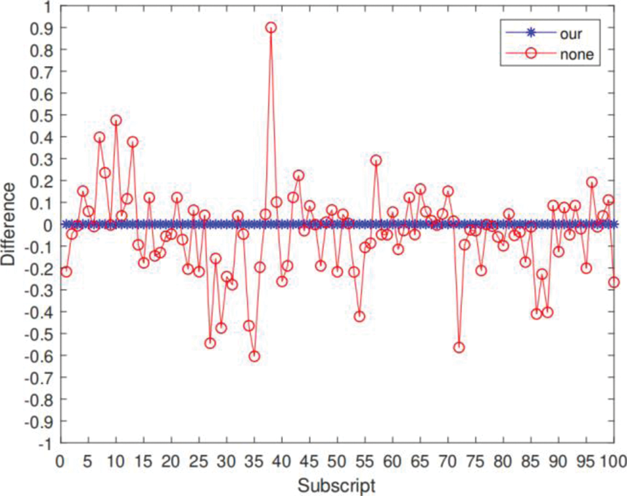
Figure 10: Vertical coordinates of the blue and red points indicate the difference in slopes of the control points on both sides of the common boundary when the C1/G1 constraint is applied and not applied, respectively

Solving partial differential equations with IGA. To demonstrate that the parameterization of target models obtained by our method can be used in IGA, we solve the Poisson problem mentioned in [17] on a target domain:

{−Δϕ=f (in Ω)ϕ=g (on ∂Ω).

The right terminal term in the Poisson equation is f=2π2sin(πx)sin(πy), since we know that the analytic solution of the equation is ϕ(x,y)=sin(πx)sin(πy). To satisfy the Dirichlet conditions g, we approximate g with boundary basis functions before solving the equation with IGA.

Based on the definition of the spline surface, the approximating numerical solution in each subdomain can be formulated as follows:

ϕh(ξ,η)=(x(ξ,η),y(ξ,η))=∑i=0m∑j=0nuijNi,j(ξ,η),

where Ni,j(ξ,η) is the product of bivariate basis functions. We need to obtain the coefficients uij, i=0,1, ⋯,m; j=0,1, ⋯, n in each subdomain, and the coefficients on common boundaries of neighboring subdomains are the same. Fig. 11 shows the exact solutions and absolute errors of our models, where we used uniform vectors for each subdomain in all of the models. More specifically, the degree of the B-splines for models in the first and fourth columns was four, and the degree of the other two models was three. The number of control points for the model in the fourth column was 12×12, and the number of control points for the other three models was 5×5.

Figure 11: The first row shows the exact solutions in different computational domains, and the second row shows the colormap of the absolute error of the solution

Limitations of algorithm. In this paper, we experimentally verified that if the target model approximates the source model after rigid transformations such as scaling, translation, and rotation or non-rigid transformations such as minor articulation and local transformation, the parameterization results of the target model obtained after the parametrization transfer meet the computational accuracy and efficiency requirements in the subsequent simulation analysis of the model. For the case when the difference between the target and original models is large, the algorithm in this paper can also yield reasonable results. Fig. 12 shows the parametrization transfer results after increasing the degree of nonlinear transformation of a wrench model. The parametrization results of the target model met the requirements of the IGA in this process for all cases, but the quality of the patches in the part with articulation will keep decreasing. Although this process produced reasonable results for all the examples presented in this paper, the optimization process cannot theoretically guarantee the complete elimination of fold-over in the patches. Thus, it cannot guarantee that the parametrization transfer results always meet the requirements of the IGA, which will be a direction of future improvement.

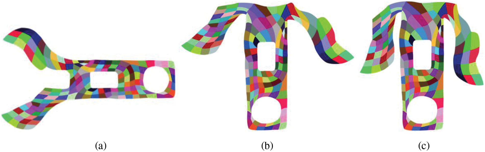
Figure 12: (a) Source model of a wrench. (b, c) Results of the parametrization transfer when the two corners of the wrench underwent constant downward transformation. The results show that even with a relatively large degree of articulation transformation, a desirable parameterization result could be produced

5  Conclusions and Future Work

We proposed a novel method to transfer the parameterization results of a model to another model with a similar shape, and the C1/G1 continuity was satisfied between adjacent patches of the target model. The parameterization results can be used in IGA and other geometry processing problems. Experiments showed that if the shape of the target model is similar to the original model, e.g., if the two models can be transformed by rotation, translation, scaling, and other rigid or articulation transformations, with a small degree of nonlinear deformation, the algorithm can obtain a more ideal parametrization transfer result. However, determining how to measure the similarity of the two shapes and the transfer result theoretically has not been defined clearly, which is a problem to be solved in the future.

Funding Statement: This work was supported by the National Natural Science Foundation of China (Grant Nos. 62072148 and U22A2033), the National Key R&D Program of China (Grant Nos. 2022YFB3303000 and 2020YFB1709402), the Zhejiang Provincial Science and Technology Program in China (Grant No. 2021C01108), the NSFC-Zhejiang Joint Fund for the Integration of Industrialization and Informatization (Grant No. U1909210), and the Fundamental Research Funds for the Provincial Universities of Zhejiang (Grant No. 490 GK219909299001-028).

Conflicts of Interest: The authors declare that they have no conflicts of interest to report regarding the present study.

References

1. Xu, G., Li, M., Mourrain, B., Rabczuk, T., Xu, J. et al. (2018). Constructing IGA-suitable planar parameterization from complex CAD boundary by domain partition and global/local optimization. Computer Methods in Applied Mechanics and Engineering, 328, 175–200. [Google Scholar]

2. Xu, G., Mourrain, B., Duvigneau, R., Galligo, A. (2011). Parameterization of computational domain in isogeometric analysis: Methods and comparison. Computer Methods in Applied Mechanics and Engineering, 200(23–24), 2021–2031. [Google Scholar]

3. Nian, X., Chen, F. (2016). Planar domain parameterization for isogeometric analysis based on Teichmüller mapping. Computer Methods in Applied Mechanics and Engineering, 311, 41–55. [Google Scholar]

4. Yuan, G. J., Liu, H., Su, J. P., Fu, X. M. (2021). Computing planar and volumetric B-spline parameterizations for IGA by robust mapping fitting. Computer Aided Geometric Design, 86, 101968. [Google Scholar]

5. Xu, J., Chen, F., Deng, J. (2015). Two-dimensional domain decomposition based on skeleton computation for parameterization and isogeometric analysis. Computer Methods in Applied Mechanics and Engineering, 284, 541–555. [Google Scholar]

6. Xiao, S., Kang, H., Fu, X. M., Chen, F. (2018). Computing IGA-suitable planar parameterizations by PolySquareenhanced domain partition. Computer Aided Geometric Design, 62, 29–43. [Google Scholar]

7. Kim, V. G., Lipman, Y., Funkhouser, T. (2011). Blended intrinsic maps. ACM Transactions on Graphics, 30(4), 1–12. [Google Scholar]

8. Vestner, M., Lähner, Z., Boyarski, A., Litany, O., Slossberg, R. et al. (2017). Efficient deformable shape correspondence via kernel matching. 2017 International Conference on 3D Vision (3DV), pp. 517–526. Qingdao, China. [Google Scholar]

9. Zheng, X., Wen, C., Lei, N., Ma, M., Gu, X. (2017). Surface registration via foliation. Proceedings of the IEEE International Conference on Computer Vision, pp. 938–947. Venice. [Google Scholar]

10. Aigerman, N., Poranne, R., Lipman, Y. (2014). Lifted bijections for low distortion surface mappings. ACM Transactions on Graphics, 33(4), 1–12. [Google Scholar]

11. Aigerman, N., Lipman, Y. (2015). Orbifold tutte embeddings. ACM Transactions on Graphics, 34(6), 1–12. [Google Scholar]

12. Aigerman, N., Kovalsky, S. V., Lipman, Y. (2017). Spherical orbifold tutte embeddings. ACM Transactions on Graphics, 36(4), 1–13. [Google Scholar]

13. Baden, A., Crane, K., Kazhdan, M. (2018). Möbius registration. Computer Graphics Forum, 37, 211–220. [Google Scholar]

14. Panozzo, D., Baran, I., Diamanti, O., Sorkine-Hornung, O. (2013). Weighted averages on surfaces. ACM Transactions on Graphics, 32(4), 1–12. [Google Scholar]

15. Ezuz, D., Solomon, J., Ben-Chen, M. (2019). Reversible harmonic maps between discrete surfaces. ACM Transactions on Graphics, 38(2), 1–12. [Google Scholar]

16. Su, J. P., Fu, X. M., Liu, L. (2019). Practical foldover-free volumetric mapping construction. Computer Graphics Forum, 38, 287–297. [Google Scholar]

17. Wang, S., Ren, J., Fang, X., Lin, H., Xu, G. et al. (2022). IGA-suitable planar parameterization with patch structure simplification of closed-form polysquare. Computer Methods in Applied Mechanics and Engineering, 392, 114678. [Google Scholar]