
 Submit a Paper
 Propose a Special lssue
 Open Access
ARTICLE

Multi-Attribute Group Decision-Making Method under Spherical Fuzzy Bipolar Soft Expert Framework with Its Application
1
Department of Mathematics, Faculty of Science and Arts, Mahayl Assir, King Khalid University, Abha, Saudi Arabia
2
Department of Mathematics and Computer, Faculty of Science, Ibb University, Ibb, Yemen
3
Department of Mathematics, Division of Science and Technology, University of Education, Lahore, Pakistan
* Corresponding Author: Ghous Ali. Email:
(This article belongs to the Special Issue: Decision making Modeling, Methods and Applications of Advanced Fuzzy Theory in Engineering and Science)
Computer Modeling in Engineering & Sciences 2023, 137(2), 1891-1936. https://doi.org/10.32604/cmes.2023.027844
Received 17 November 2022; Accepted 14 February 2023; Issue published 26 June 2023
 View Full Text
 Download PDF
Abstract
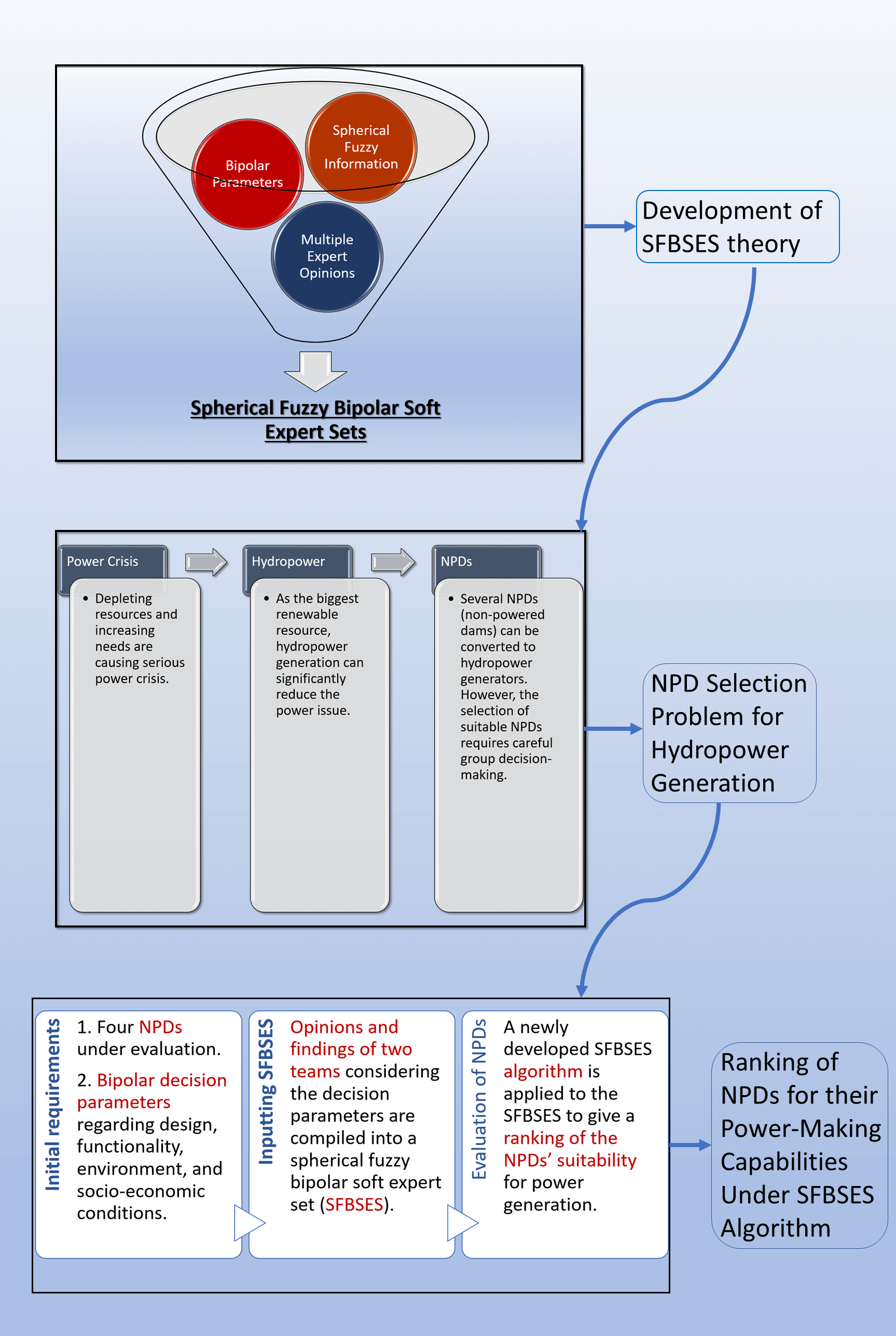
Spherical fuzzy soft expert set (SFSES) theory blends the perks of spherical fuzzy sets and group decision-making into a unified approach. It allows solutions to highly complicated uncertainties and ambiguities under the unbiased supervision and group decision-making of multiple experts. However, SFSES theory has some deficiencies such as the inability to interpret and portray the bipolarity of decision-parameters. This work highlights and overcomes these limitations by introducing the novel spherical fuzzy bipolar soft expert sets (SFBSESs) as a powerful hybridization of spherical fuzzy set theory with bipolar soft expert sets (BSESs). Followed by the development of certain set-theoretic operations and properties of the proposed model, important problems, including the selection of non-powered dam (NPD) sites for hydropower conversion are discussed and solved under the proposed approach. These problems mainly focus on the need for an efficient tool capable of considering the bipolarity of parameters, complicated ambiguities, and multiple opinions. Supporting the new approach by a detailed comparative analysis, it is concluded that the proposed model is more comprehensive and reliable for multi-attribute group decisionmaking (MAGDM) than the previous tools, particularly considering the bipolarity of parameters under SFSES environment.Graphic Abstract
Keywords
Considering complicated issues like falling economies, fastly spreading epidemics, global carbon footprints, environmental pollution, severe weather conditions due to rapid climate changes, energy crises, and depleting resources, many uncertainties arise in making profitable policy decisions. Concerning these issues, including the decision for an optimum object, ranking the policies concerning their possible outcomes, and predicting based on available data, decision sciences offer tools capable of handling vagueness and uncertainties effectively. Following the very first uncertainty theory of probability that was developed during the 16
Concerning the uncertainties and partial information in the problems, classical set theories could not help in decision-making. To tackle these situations, Zadeh [1] revolutionized the decision sciences with his invention of fuzzy sets. These fuzzy sets allowed the solutions to uncertain problems by considering partiality of truth rather than perfect truth and perfect false. In contrast to classical sets with memberships 0 and 1 proclaiming only absolute conditions, Zadeh [1] assumed belongingness degrees for alternatives in the interval [0,1]. Therefore, the fuzzy sets provide information about the partial belongingness of things, contrary to their presence or absence. This revolutionary idea motivated many researchers to develop and base their decision-making models using fuzzy sets [2].
The fuzzy sets discuss only the membership of agreement about an object and therefore fail to solve problems that must consider both the belongingness and non-belongingness degrees. To incorporate disagreement degrees for such issues, Atanassov [3] came up with the intuitionistic fuzzy set (IFS) theory. These IFSs took both belongingness and non-belongingness degrees into consideration, corresponding to the decision-maker’s opinion about agreement and disagreement with a particular perspective, including the restriction that the sum of both these degrees must not exceed unity. Later, this model proved unsuccessful in handling problems with these two membership degrees summing up to values above one. For such problems, Atanassov [4] extended his IFSs to IFSs of the second type (type-2 IFSs). These type-2 IFSs allowed the sums of the belongingness and non-belongingness degrees to exceed unity with the new constraint that the sum of squares of these two degrees must keep from 0 to 1. Identical to these type-2 IFSs, Yager [5] introduced the Pythagorean fuzzy set (PyFS) model as an extension of the IFSs. Later, many decision-makers embraced this generalized form to develop more powerful hybrid decision models. Deveci et al. [6] provided a survey on the applications of PyFSs. Recently, Habib et al. [7] used PyFS-based multi-criteria decision-making (MCDM) methods for diagnosing the risk of eight different types of cancer in children.
Adding to the above scenarios, the situations like elections, surveys, and polls, often ask for a neutral opinion as well. For instance, a survey may ask for positive, negative and neutral opinions about various points. These scenarios require a third degree, i.e., the neutral membership degree in addition to the two prior discussed evaluation degrees. Considering such situations, Coung et al. [8–10] proposed picture fuzzy sets (PFSs) by considering negative, positive, and neutral membership degrees reflecting the disagreement, agreement, and neutrality in the decision-maker’s opinion. Currently, Singh et al. [11] studied applications of picture fuzzy correlation coefficients. A drawback of these PFSs is that they are not capable to tackle problems with negative, positive, and neutral memberships summing above unity. Considering the problems with this sum exceeding unity, Kahraman et al. [12] initiated the notion of spherical fuzzy sets (SFSs) by smoothening the restriction of the picture fuzzy sets with the condition that the sum of squares of positive, neutral, and negative memberships ranges from 0 to 1. Thus, it provided a generalization for the previous models. Later, Gündogdu et al. [13] proposed a TOPSIS (technique of order preference similarity to the ideal solution) approach for dealing with decision-making applications using generalized SFSs. Akram et al. [14] discussed a group decision-making mechanism based on the complex spherical fuzzy VIKOR method. Recently, Donyatalab et al. [15] introduced their new spherical fuzzy similarity and distance measures, and discussed their applicability in the diagnosis of diseases. Wang et al. [16] discussed a detailed site selection application for offshore wind power plants using SFSs under two-stage MCDM. Similarly, in the past few years, SFSs have been employed to tackle many decision-making situations [17–21]. Fig. 1 compares the IFSs, PyFSs, PFSs, and SFSs in a graphical manner.
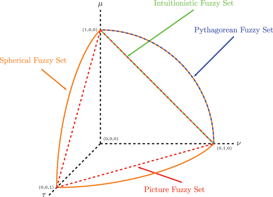
Figure 1: Pictorial representation of IFS, PyFS, PFS, and SFS
One common limitation of all the above-discussed models is that they consider opinions respective to only a single parameter. However, generally, the decision-making problems are based on choices keeping multiple parameters under consideration. To integrate multiple parameters in one place, Molodtsov [22] introduced soft sets as the parameterized families of the provided universe of discourse. Maji et al. [23] discussed the decision-making applications of soft sets. Inspired by the parameterizing capability of soft sets, many hybrid structures have been developed in the last two decades by the combination of multiple uncertainty theories with soft sets. For instance, Sun et al. [24] combined linguistic variables with soft set theory to form linguistic valued soft sets with linguistic values. Perveen et al. [25] developed a spherical fuzzy soft set (SFSS) model by combining SFSs with soft sets. Guleria et al. [26] introduced T-spherical fuzzy soft sets (T-SFSSs) as the hybridization of T-SFSs with soft sets. Akram et al. [27] provided TOPSIS approach for dealing with complex spherical fuzzy information. In addition, complex spherical Dombi fuzzy aggregation operators were initiated by Akram et al. [28]. Zahid et al. [29] introduced an ELECTRE-based method using complex spherical fuzzy information for group decision-making. Akram et al. [30] discussed the decision-making applications of complex spherical fuzzy N-soft sets. Recently, Yang et al. [31] introduced T-spherical fuzzy Bonferroni mean operators and discussed their applications in multi-criteria decision-making. Manna et al. [32] presented an MADM method under a complex neutrosophic environment. Adeel et al. [33] provided a decision-making analysis using the ELECTRE-I approach under hesitant fuzzy N-soft sets. Some other recent works include [34–38]. Very recently, Liu et al. [39] presented a fuzzy soft expert prediction system to diagnose the COVID-19 (Coronavirus disease 2019).
The highly demanding problems, particularly those affecting important future considerations, require group decision-making. The previously discussed models are restricted to a single expert’s opinions and are not capable of making group decisions efficiently. To fulfill this requirement, Alkhazaleh et al. [40] developed soft expert sets (SESs), capable of dealing with multiple experts’ opinions in one place. Later, Alkhazaleh et al. [41] combined fuzzy sets with SESs and presented fuzzy soft expert sets (FSESs). Considering the group decision-making capabilities of SESs, lots of recent works focused on the hybridizations and improvements based on these sets. Bashir et al. [42] introduced possibility fuzzy soft expert sets by providing possibility degrees along with the fuzzy memberships. Fuzzy parameterized soft expert sets developed by Bashir et al. [43] allowed preference of parameters by assigning fuzzy values to parameters. Fusing SFSs with SESs, Perveen et al. [44] established spherical fuzzy-SES (SFSES) model and discussed its MAGDM applications. Combining the rating-based decision qualities with SFSs and SESs, Akram et al. [45] presented spherical fuzzy N-SESs and explored their MAGDM problems in survey-based election prediction and product review.
In considering the uncertainties with multiple parameters, many decision-making problems arise with bipolar parameters interrelated symmetrically. For instance, a medical test can be sensitive or specific, a person can be young or old, and a student can be dull or intelligent. Such dual behavior of parameters requires tools eligible to manage and depict this bipolarity. Shabir et al. [46] introduced bipolar soft sets (BSSs) composed of two soft sets; one based on the set of parameters, and the other based upon the not-set of parameters (one set contains the parameters opposite to those in the other set). Ali et al. [47] presented bipolar-SESs (BSESs) as the fusion of BSSs with SESs, and discussed their decision-making applications. Further extending BSESs for uncertain situations, Ali et al. [48] initiated fuzzy BSESs (FBSESs) and discussed their MAGDM applications. Recently, Ali et al. [49] ranked the fish passage designs for a hydropower project based on spherical fuzzy-BSSs (SFBSSs). Many other models based on BSSs came out in the recent years, e.g., q-rung orthopair fuzzy BSSs (qROFBSSs) [50]. Table 1 provides the list of abbreviations used in the paper. Table 2 represents the list of frequently used symbols throughout the work.


The complications arising in the emerging decision problems considering the energy crisis and depleting energy resources ask for more efficient decision-making powered by much stronger and comprehensive tools. For instance, hydropower is a non-depleting carbon-free renewable energy resource bearing maximum potential as compared to all other renewable energy resources. However, all dams and water reservoirs are not dedicated to hydropower generation. Hadjerioua et al. [51] provided a detailed estimation of energy capacity at non-powered dams (NPDs) in the United States and their report signifies the importance of NPDs capable of generating electricity and adding to hydropower generation through proper installations and considerations. The point is that all NPDs cannot generate electricity, and the selection of NPDs capable of hydropower generation requires complicated MAGDM. This demands considering spherical fuzzy opinions of multiple experts (or teams) for tackling the uncertainties governed by the bipolar parameters depicting favoring and symmetrically non-favoring factors. Such a problem is unsolvable by the existing theories, including SFSESs, BSESs, SFBSSs, etc. That is why, this work focuses on the development of a novel hybrid model named spherical fuzzy bipolar soft expert sets or SFBSESs as a combination of SFSs [12] and BSESs [47], and then the ranking of the NPDs’ suitability for hydropower installations under SFBSESs. Table 3 gives an overview of the considerations taken into account by multiple decision-models. It can be clearly observed that the innovative proposed model considers maximum dependencies affecting the decision-making, hence leaving negligible chances of error as compared to all of the pre-existing tools.

1.1 Motivations and Contributions
The motivations of this work are provided as below:
1. The possible contribution of NPDs in hydropower generation (as discussed in [51]) is very important in minimizing the power crisis. However, a lot of positive and negative factors considering the infrastructure, location, politics, etc., ask for efficient MAGDM decision-making under the expertise of multiple experts.
2. The existing models like PFSs [8–10], SFSSs [25] and SFSESs [44] offer reliable solutions to uncertainties by considering the degrees of positive, negative and neutral opinions. However, all of these are incapable to discuss the bipolarity of decision-parameters, therefore unreliable to solve problems governed by symmetrically opposing factors.
3. Models based on BSSs [46] like BSESs [47], FBSESs [48] and qROFBSSs [50] efficiently differentiate between the bipolar decision-parameters, however all these models fail to consider the degree of neutrality when solving uncertain problems.
4. The MAGDM capabilities of SESs [40] for dealing complex situations considering multiple experts offer more reliable and unbiased solutions. Most of the existing works as discussed in Table 3 lack this capability.
The main contributions of this paper are given as below:
1. Combining the uncertain decision-making properties of SFSs [12] with the group decision-making capabilities of BSESs [47], a hybrid model is presented with higher performance when examining MAGDM problems in spherical fuzzy environment under bipolar parameters. This hybridization allows group decision considerations of 3 dimensional opinions regarding the uncertainties in problems governed by symmetrically opposing parameters.
2. The algebraic characteristics and operations of the initiated structure are discussed and illustrated through numerical examples. These operations depict inclusion and aggregation techniques in multiple ways for combining and comparing between different sets of SFBSE information.
3. A powerful MAGDM algorithm under SFBSESs is proposed. This enhanced algorithm combines the previous algorithms (as in [44,48,49]) to tackle their limitations as discussed in the literature. Consequently, many problems unsolvable by the previous works due to the loss of information will now seek their solutions reliably.
4. Considering the importance of NPDs in improving the power generation and the complicated uncertainties arising in appropriate site selection procedure for hydropower conversion, a model NPDs site selection problem is modeled using SFBSES and solved under the proposed algorithm. This model application gives an insight about how equally complicated actual problems can be solved with the presented method.
This paper is organized as:
• Section 2 recalls the preliminary definitions and related notions that will be utilized in the further development of this work.
• Section 3 presents SFBSESs along with their algebraic properties and fundamental operations, including subset-hood, complement, intersection (restricted and extended), union (restricted and extended), SFBSE-AND operation and SFBSE-OR operation.
• Section 4 explores an application of the SFBSESs, i.e., ranking of NPDs regarding suitabilities for hydropower generation, and its solution under the novel algorithm proposed for SFBSESs.
• Section 5 discusses the advantages of proposed MAGDM hybrid model by comparing it with the existing models, and debates the possible limitations.
• At last, Section 6 gives some conclusive remarks and possible future extensions of the presented method.
This section recalls important notions useful in the development of this paper. Let us start with the definition of spherical fuzzy sets (or SFSs).
Definition 2.1.[12] For
where
The set
Some important properties and operations of the SFSs are listed as follows:
Definition 2.2.[12] Suppose
1.
2.
3.
4.
5.
The next definition calls back the notion of spherical fuzzy soft sets (or SFSSs).
Definition 2.3.[25] Suppose
where
Some important definitions for SFSSs are recalled below, which will help in development of the new MAGDM algorithm.
Definition 2.4.[25] Consider a SFSS
1. Mid-level Threshold Function (
The mapping
such that
The mid-level soft set of
2. Top-bottom-bottom-level Threshold Function (
The mapping
such that
The top-bottom-bottom-level (tbb-level) soft set of
3. Bottom-bottom-bottom-level Threshold Function (
The mapping
such that
The bottom-bottom-bottom-level (bbb-level) soft set of
4. Med-level Threshold Function (
The mapping
such that
Here
To deal with MAGDM problems concerning spherical fuzzy information, the existing notion of spherical fuzzy soft expert set (or SFSES) is defined as below:
Definition 2.6.[44] Suppose
The following definition reviews the notion of bipolar soft sets:
Definition 2.7.[46] Consider
The set
whereas
The following definition recalls the concept of bipolar soft expert sets (or BSESs), which are capable to handle bipolarity in MAGDM situations:
Definition 2.8.[47] Consider
Here,
3 Spherical Fuzzy Bipolar Soft Expert Sets
This section first introduces the concepts of spherical fuzzy bipolar soft expert sets (or SFBSESs), and then discusses the necessary operations and properties. The following defines the novel SFBSESs.
Definition 3.1.Let
Here,
such that
The following example illustrates how SFBSESs can be used in modeling and depicting complicated decision-making situations.
Example 3.1.Consider an international bank that is trying to increase its business by effectively implementing the foreign exchange strategies. To ensure it happens, the bank needs a strong analysis as well as a valuable and efficient prediction method for the currency exchanges. However, this is a difficult and complex task. To deal with this, the bank calls its market analysts and currency exchangers to ensure the maximum profit and least risk.
These forex experts propose three strategies already working in the market, comprising the set
Tables 4 and 5 represent the formulated SFBSES in terms of


whereas Table 7 represents the general form of the single tabular format for SFBSESs. It can be observed from Table 6, how the opinions of the experts differ from each other according to their expertise. This flexible opinion set provides better insight and analysis for the complex scenario and hence offers unbiased and more reliable handling of the decision problem under spherical fuzzy information, while considering the bipolarity of the affecting parameters.

Remark 3.1.The above example demonstrates a problem that could not be fully represented by any of the previous tools. SFSESs fail to consider the bipolarity of parameters, BSESs fail to tackle the complicated spherical fuzzy uncertainties in the problem and SFBSSs cannot manage opinions of multiple experts in a single place. This highlights the need for the proposed work which unifies all these models into a single model providing superior uncertainty handling under multiple experts while considering the bipolar behavior of governing decision-parameters.
The coming definition defines the SFBSE subset.
Definition 3.2.A SFBSES
1.
2.
3.
Remark 3.2. Analytically, a SFBSE-subset shows lesser suitability in a decision scenario as compared to that shown by the respective super-set. This lesser suitability or deprived favorability is expressed in the form of missing considerations (relatively fewer decision-parameters) accompanied by lower supporting membership degrees. For instance, two SFBSESs are reported for a firm’s performance at different times with the second set being the subset of the first set. The subset relation then indicates a decline in the firm’s performance with increasing time.
Example 3.2.Recall Example 3.1. Suppose that two SFBSESs
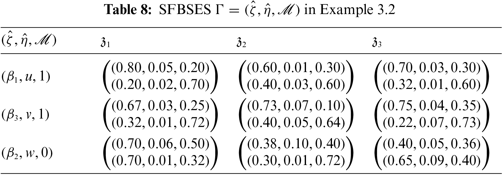

Clearly,
Definition 3.3.Any two SFBSESs
Based on the concept of complement of SFSs, the complement of a SFBSES is defined as:
Definition 3.4.The complement of SFBSESExample 3.3.Consider the SFBSES

Proposition 3.1.Let
1.
1. By Definition 3.4,
for all
Thus,
The relative null and relative absolute SFBSESs over
Definition 3.5.A SFBSES
and
Similarly, a SFBSES
and
Proposition 3.2.Consider the relative null and relative absolute SFBSESs, i.e.,
1.
2.
Proof. The proofs are obvious from the Definitions 3.4 and 3.5.
The following Definition 3.6 explains the concepts of agree and disagree SFBSESs:
Definition 3.6.The agree SFBSES
for all
for all
Example 3.4.Consider the SFBSES


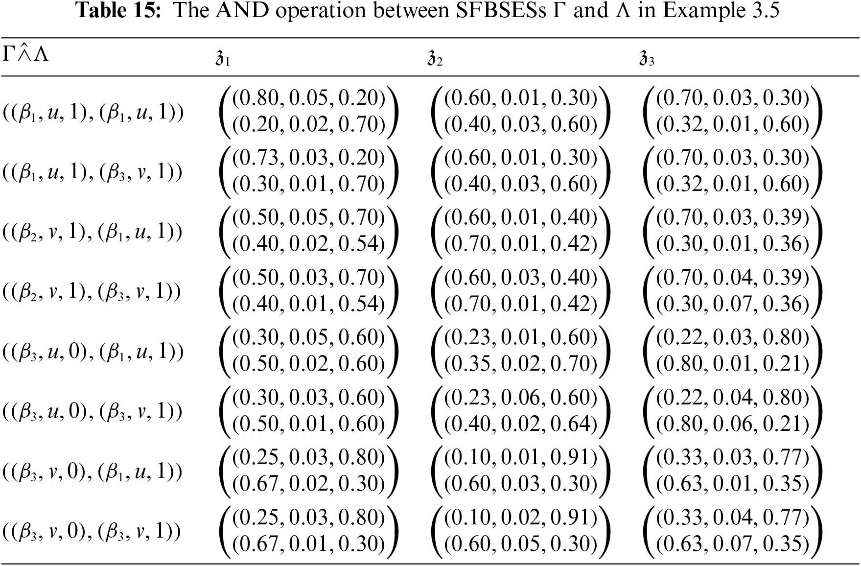
The following definition provide the idea of AND operation between SFBSESs:
Definition 3.7.For two SFBSESs
such that
The next definition gives the OR operation between SFBSESs.
Definition 3.8.For two SFBSESs
such that
The following example provides an illustration of the AND and OR operations between two SFBSESs:
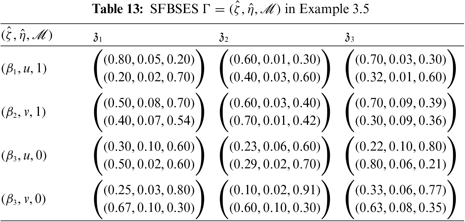
Example 3.5.Reconsider Example 3.1. For


Proposition 3.3.Let
1.
2.
1. Let
where
and
For all
where
Thus,
Let
where
and
For all
where
Thus,
Proposition 3.4.Let
1.
2.
3.
4.
Proof.
1. By Definition 3.7, we have
Hence proved.
2. By Definition 3.8, we have
Hence proved.
The remaining proofs are similar as above parts.
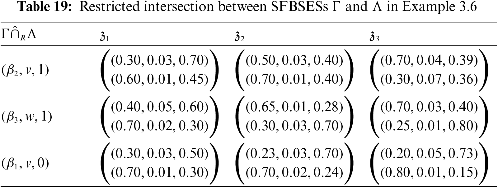
The SFBSE restricted intersection and union are defined in the following Definitions 3.9 and 3.10, respectively.
Definition 3.9.The SFBSE restricted intersection among the SFBSESs
such that
Definition 3.10.The SFBSE restricted union among the SFBSESs
such that
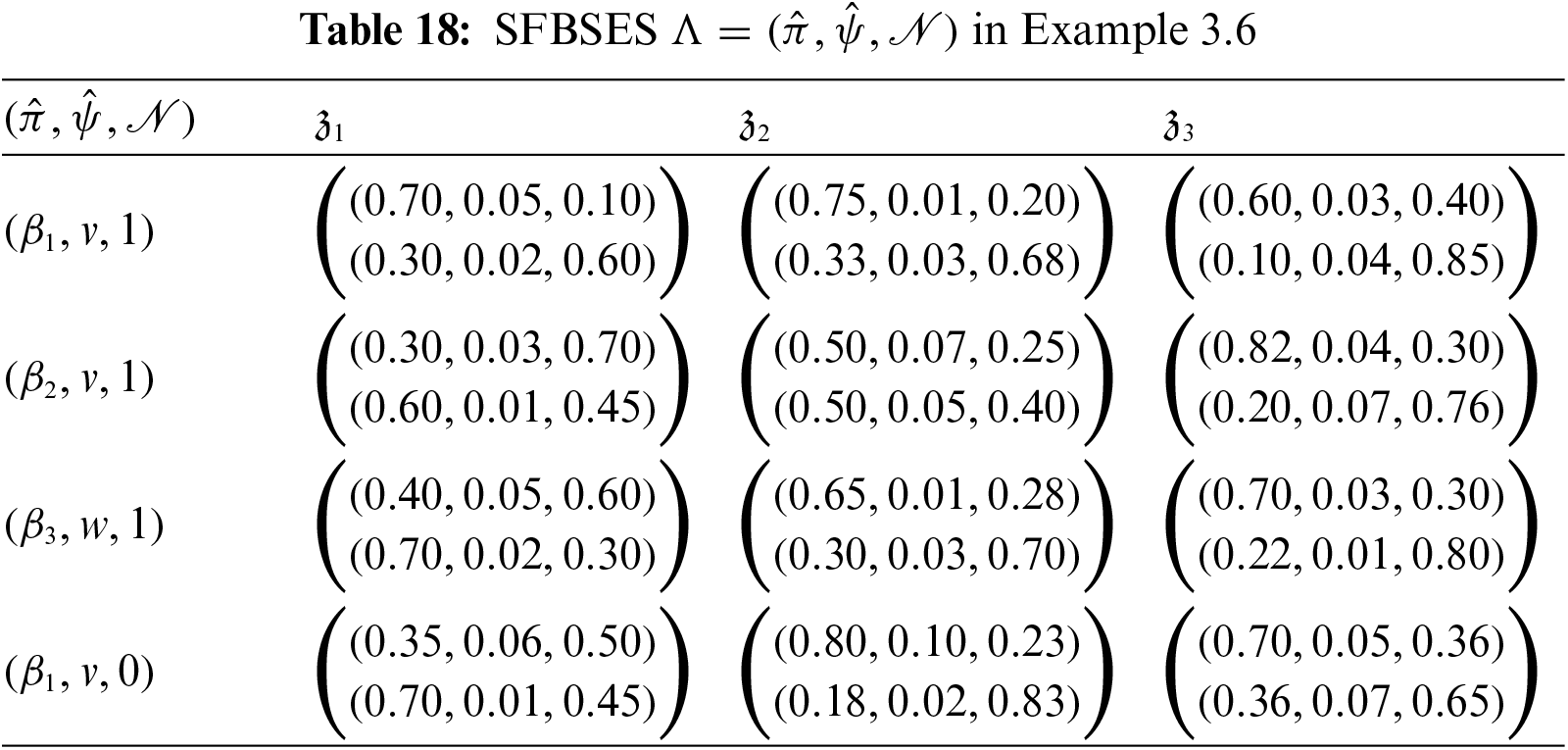
Example 3.6.Reconsider Example 3.1 again. Consider the SFBSESs corresponding to the sets


Proposition 3.5. Let
1.
2.
Proof.
1. Consider
such that
Similarly,
such that
This implies that
2. Consider
such that
Similarly,
such that
This implies that
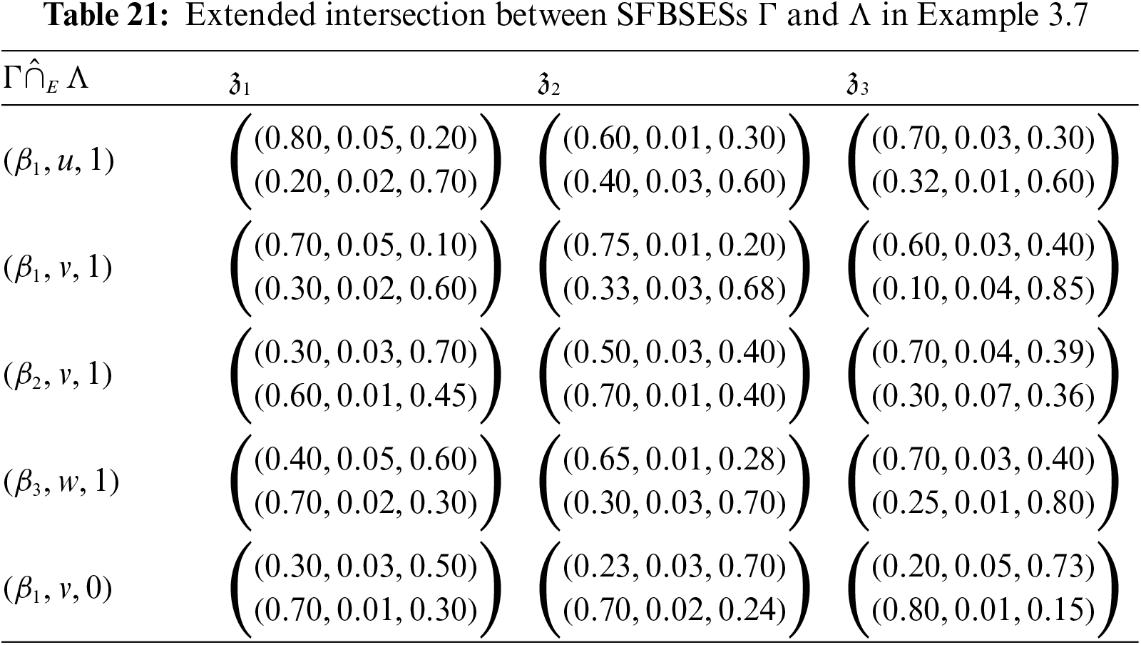
Definition 3.11.The SFBSE extended intersection among the SFBSESs
such that
Definition 3.12.The SFBSE extended union among the SFBSESs
such that
Example 3.7.Reconsider the SFBSESs

1.
2.
3.
4.
5.
6.
Proof.
1. Let
Eliminating the trivial cases, and considering only
Similarly,
This implies that
The remaining parts can be proved using similar arguments.
Proposition 3.7.Let
1.
2.
3.
4.
5.
Proof. The proofs can be directly deduced from Definitions 3.8 to 3.12.
4 Application of SFBSESs in MAGDM Environmental Problem
In this section, we present an application of SFBSESs regarding the ranking of non-powered dams to be powered in the future. Before going to the application and presenting the algorithm, we define some important notions as follows:
Remark 4.1.Note that the SFSESs
Remark 4.2.The SES tables representing the level favor SES
Remark 4.3.The SES table representing the focus-level SES
The agree and disagree subsets of the focus-level SES are defined as follows:
Definition 4.1.The agree focus-level SES
Similarly, the disagree focus-level SES
We now present an algorithm based on SFBSES for ranking alternatives considering an MAGDM problem as follows:
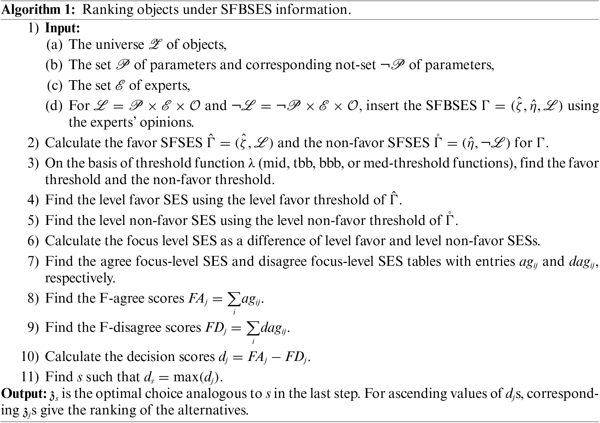
Fig. 2 gives a flowchart for the above algorithm.
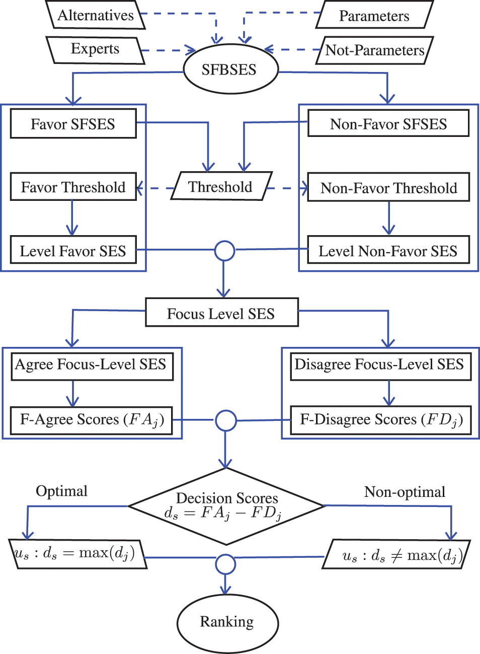
Figure 2: Multi-attribute group decision-making under SFBSESs
Example 4.1. Ranking of non-powered dams’ suitability for a hydroelectric project:
With the continuously increasing population, adoption of technologies, electricity-powered appliances, industries, vehicles, and more, the need for power production is ever increasing, leading to massive usage of resources consumed in the power-generation process. For many years, this power has been generated over the globe using power-generation plants based on non-renewable resources such as natural gas, oil, coal, etc. Unfortunately, these resources are non-renewable and depleting at rates faster than ever before. In this scenario, consideration of an alternative is mandatory to keep the power-generation procedure intact while minimizing the usage of non-renewable resources.
Renewable resources based on the sun, water, earth, wind, and nuclear energy prove very effective alternatives for the discussed scenario. These resources include solar power, wind energy, geothermal energy, nuclear power, hydropower, tidal power, bio-gas, etc. All these resources have advantages and limitations based on their setup costs, geological requirements, possible hazards, sustainability, dependence, efficiency, and more. According to recent trends, governments all over the globe are planning and working to maximize the usage of renewable resources and minimize the usage of fossil fuels for power generation. On analyzing the global renewable energy generation and consumption, it clarifies that hydropower is the most common and widely used renewable energy resource all over the globe. Due to the massive amount of water on planet Earth, this particular renewable resource can benefit more widely and efficiently by considering critical measures and improvements. As of 2020, according to the international energy agency1, hydropower reached 4418 Terawatt-hour (TWh) by generating more power than all other renewable energy resources in total.
Hydropower mainly generates using dams all over the globe, equipped with special power-generation equipment including turbines, pumps, etc. Apart from these hydroelectric projects, numerous watersheds, dams, and reservoirs do not yet intend to produce electricity. Such structures are mainly devoted to water storage, flood control, recreational activities, and navigation. These non-powered dams (NPDs) are much more in number than powered dams and constitute a substantial part of the big picture. Considering only United States (US), there are around 90,000 documented dams, of which only 3% generate electricity. However, according to organizations like Oak Ridge National Laboratory (ORNL)2,3 a lot of these NPDs can be effectively used for hydropower generation. From the energy potential assessment made at US NPDs in 2012 by Hadjerioua et al. [51] under the US Department of Energy carried out by ORNL, Fig. 3 represents the NPDs in the US with hydropower potential exceeding one megawatt (MW). The blue circles indicate the NPDs have electricity generation potential with different radii corresponding to distinct capacities. It shows that NPDs can add to the power generation capacities by necessary measures and installations.

Figure 3: US NPDs with energy potential greater than 1 MW3
Every dam has its characteristics, geology, structure, and environmental and political impact. Therefore, a clear understanding of all these aspects is compulsory before hydroelectric generation. Turning NPDs into hydroelectric generators saves a great deal counting money, resources, space, and infrastructure. However, considering which NPDs are eligible for power generation and comparatively better than the other competing alternatives is demanding and requires effective decision-making. Motivated by this, the following example will consider the ranking of four NPDs with varying infrastructures, climates, geographies, and political considerations.
Consider there are four NPDs constituting the set
•
•
•
•

Figure 4: Decision parameters powering non-powered dams
Similarly, the non-favorable parameters form the set
•
•
•
•
Consider the two teams u and v act as the two experts collectively for the decision-making process, and generate a comprehensive report based on the collective team opinions in the form of a SFBSES
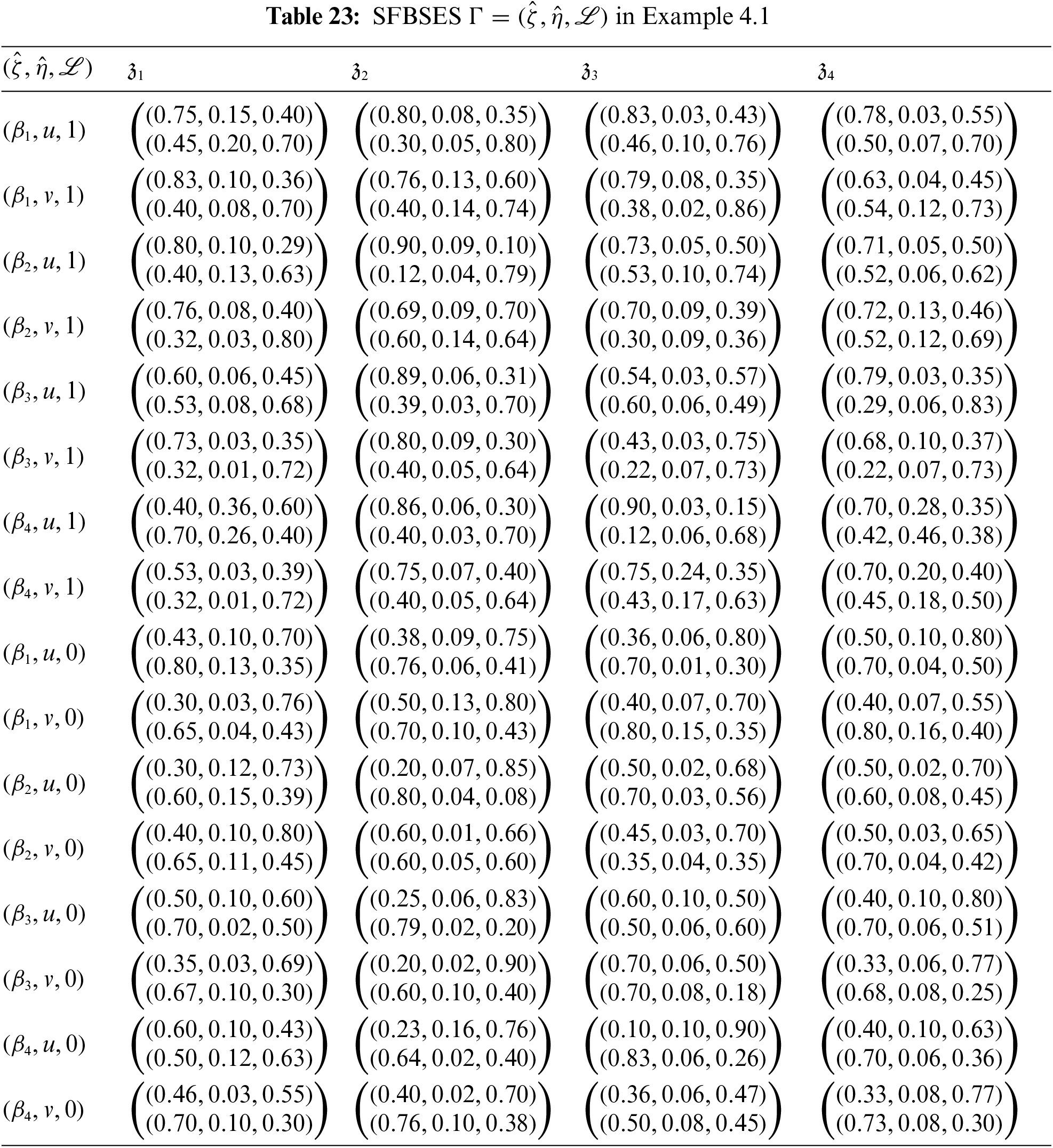
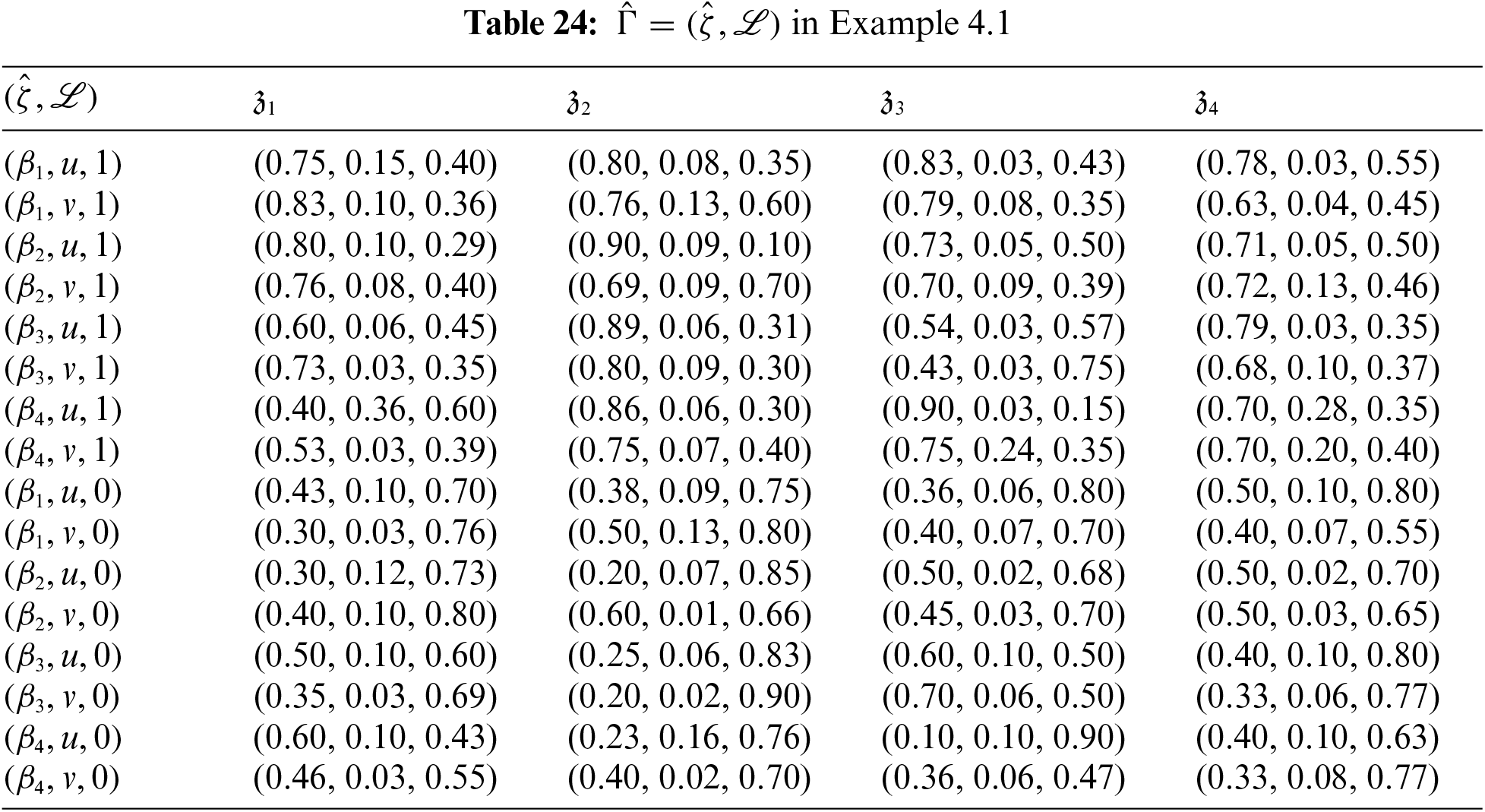
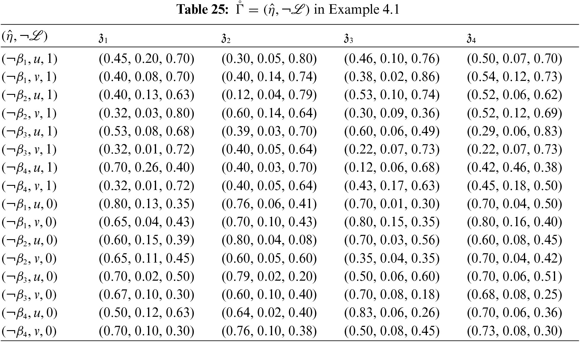
Based on the above report, the NPDs are decided to be ranked using Algorithm 1. The corresponding favor SFSES and non-favor SFSES are shown in Tables 24 and 25, respectively. Committee further decides to consider the med-level threshold for decision-making. The favor and non-favor med-level thresholds correspond to Tables 24 and 25.
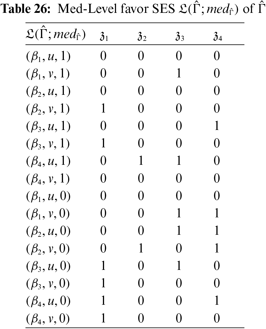
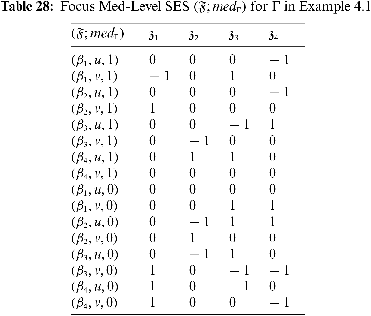
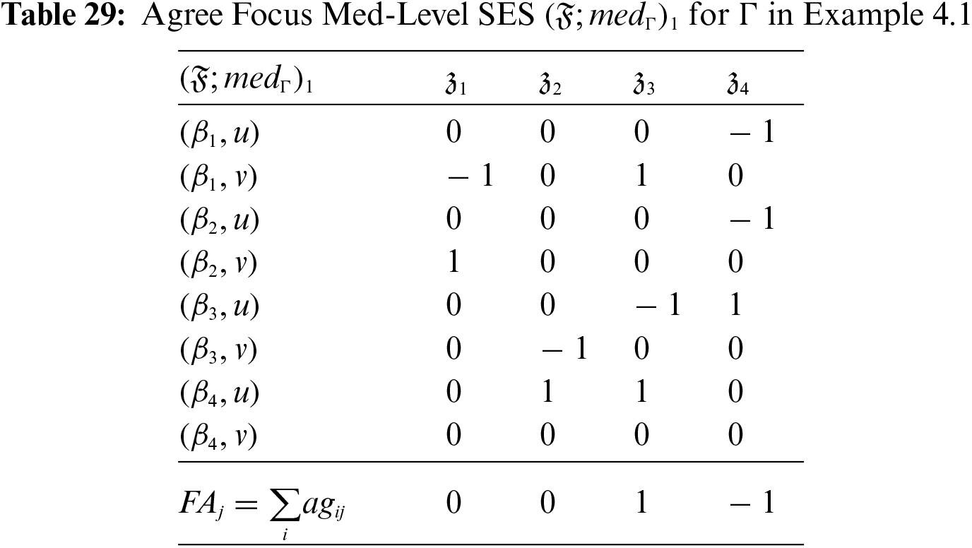
Using the above thresholds, Tables 26 and 27 represent the med-level favor SES and the med-level non-favor SES, respectively. Table 28 represents the focus med-level SES as a difference between the above two Tables. Further, the agree and disagree subsets of this focus med-level SES are shown in Tables 29 and 30, respectively.


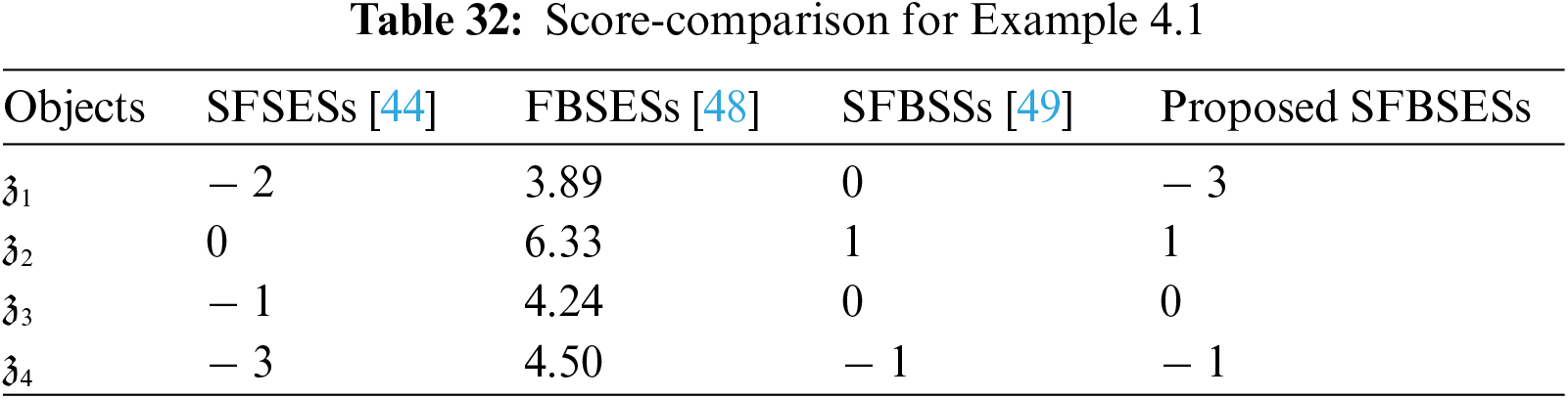
Based on the F-agree and F-disagree scores calculated in Tables 29 and 30, Table 31 represents the decision scores basing the final ranking of the NPDs as:

Hence,
This section debates the advantages and disadvantages of the proposed model, corresponding to the existing research gaps and limitations. Further, this section examines a comparative analysis of the initiated model with some recent models and proves its dominance.
Many complicated problems concerning power generation, environmental pollution, political and geological conflicts, and complex infrastructures, arise each coming day. These add to the uncertainties requiring intricate handling under corresponding experts and needing appropriate decision-making tools. Analogous to the complexity and requirements of the problems, researchers that contribute to decision-making are developing powerful decision models capable of handling specific issues unsolvable by the already existing methods. These hybridizations of different models stand very important in filling the gaps and limitations in the decision-making process and provide efficient generalized structures for the existing tools. This work initiates SFBSESs as a powerful generalization to many structures including SFSs [12], SFSSs [25], SFSESs [44], BSSs [46], BSESs [47], FBSESs [48], and SFBSSs [49]. Being the generalization, SFBSESs combine the characteristics of the antecedent models and are applicable in a much larger domain. The following list the main advantages of proposed SFBSESs:
1. The positive, neutral, and negative opinions for alternatives in the spherical fuzzy environment guarantee proper handling of complicated uncertainties.
2. The bipolar parameters depicting favorable and symmetrically non-favorable dependencies are properly distinguished in two distinct sets and then considered parallel to each other in the decision-making process.
3. Multiple experts put in their opinions at the same time minimizing the chances of biased decisions and enhancing the overall process by the merger of multiple expertise at once.
In solving the complicated MAGDM problems, both SFSESs [44] and FBSESs [48] are efficient in their respective domains. Being the combination of SFSs [12] and SESs [40], SFSESs offer solutions to MAGDM problems considering the positive, neutral, and negative opinions of decision-makers in the soft expert environment. However, SFSESs cannot distinguish between the bipolar parameters in decision-making and therefore are not very suitable for the corresponding problems. On the other hand, FBSESs as a combination of BSSs [46] and FSESs [41] offer solutions to uncertain MAGDM problems by taking the parameters’ bipolarity into account efficiently. But FBSESs fail to consider the negative and neutral memberships in the experts’ opinions. In addition, the MADM model SFBSSs [49] being a combination of SFSs [12] and BSSs [46] allows the dealing of spherical fuzzy information while considering the bipolarity of parameters. However, it is restricted to a single expert only. As the generalization of SFSESs, FBSESs, SFBSSs, and SFBSESs efficiently handle MAGDM problems by considering both the bipolarity of parameters and the neutrality and disagreement of the experts’ opinions in one place. Fig. 5 explains this difference graphically (Venn diagrams of the four sets covering the four triangular sections representing the qualities including parameterization, bipolarity, spherical fuzzy information, and multiple experts’ opinions). Table 32 represents the comparison between SFSESs, FBSESs, SFBSSs, and proposed SFBSESs by reconsidering Example 4.1 and calculating the final scores as follows:
• Using SFSESs (only considering the favorable parameters) and reducing focus level SES to level favor SES in Algorithm 1.
• Using FBSESs (only considering the degrees of agreement) and calculating the focus level SES as the difference of fuzzy SESs for favorable and non-favorable parameters in Algorithm 1.
• Using SFBSSs (fixing (u, 1) as the single expert opinion for reducing the SESs to soft sets) under the Algorithm based on SFBSSs [49].

Figure 5: SFBSESs vs. FBSESs, SFSESs, and SFBSSs
Based on the calculated final scores, the ranking orders of the alternatives are provided in Table 33. Further from Fig. 6, it is clear that ranking results are different by applying SFSESs, FBSESs, SFBSSs, and proposed SFBSESs. When using SFSESs [44], the ranking orders deviate from those, obtained by SFBSESs in the 3rd and 4th positions. With FBSESs [48], the 2nd and 3rd ranks get shuffled compared to those with SFBSESs. In addition, the SFBSSs [49] fail to make a distinction between the 2nd and 3rd rank. These deviations from the results obtained in Example 4.1 indicate the possibility of errors in making decisions by neglecting the bipolarity, ignoring the neutrality and disagreement memberships, or basing the decisions on a single expert’s opinions. Hence, it advocates that the proposed SFBSESs are more applicable and accurate than the previous models. The reduction of SFBSESs to SFSESs, FBSESs, and SFBSSs yields the same optimal solution, whereas the overall ranking provided by SFBSESs is relatively more clear and comprehensive. This proves that the proposed work is more robust and reliable relatively.
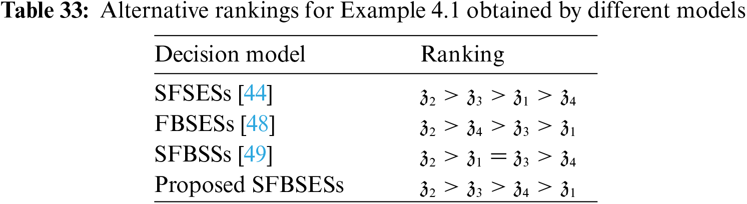
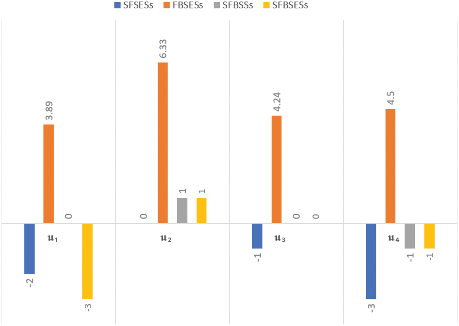
Figure 6: Scores comparison by SFSESs, FBSESs and SFBSESs
This subsection discusses the limitations and difficulties in the decision-making process by using the initiated model and algorithm. One of the flaws of the proposed model comes from its parent model SFSs, i.e., the sum of square of the degrees of agreement, disagreement, and neutrality must lie between 0 and 1. It limits the proposed model from operating in problems with this sum exceeding unity. This limitation can be managed by further extending the model using T-spherical fuzzy sets. Another ambiguity lies in the selection of threshold functions, where one may give a relatively different outcome than the others. However, the optimal selections generally remain the same. For this purpose, the decision-makers should choose the threshold functions in relevance to the data variations. Further, the lengthy algorithm and massive data make the decision process tiresome. The computing software like MATLAB and Mathematica, can be used to facilitate the implementation of the proposed algorithm. Similar to all other tools, the proposed work is also not completely perfect in itself, and particular extensions and alterations in the future may address the imperfections specifically.
6 Conclusive Remarks and Future Directions
Complicated problems, including global warming, energy crises, environmental pollution, depleting resources, and unstable economies require stakeholders, experts, and administrators to group together for seeking reliable solutions. Spherical fuzzy soft expert sets (SFSESs) [44] can efficiently deal with such uncertain MAGDM problems by considering the positive, neutral, and negative membership degrees of multiple experts’ opinions in one place. However, SFSESs fail to deal with the bipolarity of decision-parameters and hence fail to handle situations affected by parameters depicting bipolar behavior. This limitation asks for tools capable of dealing with bipolar nature problems requiring the high complexity addressable by SFSES theory. To address this requirement, we presented the novel hybrid spherical fuzzy bipolar soft expert sets (SFBSESs) by the fusion of spherical fuzzy sets [12] and bipolar soft expert sets [47]. We discussed the algebraic properties and operations of the proposed model and demonstrated these operations with numerical examples. Considering the importance of hydropower in global energy requirements and the possibility to convert certain NPD (non-powered dam) sites to hydropower dams, we presented a SFBSES-based ranking application with four NPDs advised by the two teams regarding important bipolar decision parameters in Example 4.1. The comparison section provided a detailed sensitivity analysis between FBSESs [48], SFSESs [44], and proposed SFBSESs, proving our work to be more reliable, accurate, and applicable than the pre-existing works. Being capable of dealing with maximum conditions depicting the problems and as a generalization of the previous models, SFBSESs are more robust, efficient, and comprehensive. In a nutshell, SFBSESs offer more reliable solutions to society’s complicated group decision-making problems.
Opposed to the discussed advantages, the limitations portion indicated the difficulties and restrictions concerned with the proposed model, i.e., the applicability domain restricted by the memberships’ sum condition, and the selection of the most suitable threshold function. In the future, we look forward to extending this work to the following:
• Linguistic spherical fuzzy bipolar soft expert sets using [24].
• Complex neutrosophic bipolar soft expert sets using [32].
• Possibility spherical fuzzy bipolar soft expert sets using [42].
• Fuzzy parameterized spherical fuzzy soft expert sets using [43].
• Spherical fuzzy bipolar N-soft expert sets using [45].
Funding Statement: The authors extend their appreciation to the Deanship of Scientific Research at King Khalid University for funding this work through the Large Group Research Project under Grant Number (R.G.P.2/181/44).
Conflicts of Interest: The authors declare that they have no conflicts of interest to report regarding the present study.
1https://www.iea.org/reports/hydropower.
3https://hydrosource.ornl.gov/maps.
References
1. Zadeh, L. A. (1965). Fuzzy sets. Information and Control, 8(3), 338–353. https://doi.org/10.1016/S0019-9958(65)90241-X [Google Scholar] [CrossRef]
2. Maiers, J., Sherif, Y. S. (1985). Applications of fuzzy set theory. IEEE Transactions on Systems, Man, and Cybernetics, 1(1), 175–189. https://doi.org/10.1109/TSMC.1985.6313408 [Google Scholar] [CrossRef]
3. Atanassov, K. T. (1986). Intuitionistic fuzzy sets. Fuzzy Sets and Systems, 20(1), 87–96. https://doi.org/10.1016/S0165-0114(86)80034-3 [Google Scholar] [CrossRef]
4. Atanassov, K. T. (1999). Other extensions of intuitionistic fuzzy sets. In: Intuitionistic fuzzy sets 1999, pp. 179–198. Physica, Heidelberg: Springer. [Google Scholar]
5. Yager, R. R. (2013). Pythagorean fuzzy subsets. 2013 Joint IFSA World Congress and NAFIPS Annual Meeting (IFSA/NAFIPS), pp. 57–61. Edmonton, AB, Canada. https://doi.org/10.1109/IFSA-NAFIPS.2013.6608375 [Google Scholar] [CrossRef]
6. Deveci, M., Eriskin, L., Karatas, M. (2021). A survey on recent applications of Pythagorean fuzzy sets: A state-of-the-art survey between 2013 and 2020. In: Garg, H. (Ed.Pythagorean fuzzy sets. Singapore: Springer. https://doi.org/10.1007/978-981-16-1989-2_1 [Google Scholar] [CrossRef]
7. Habib, S., Akram, M., Al-Shamiri, M. M. A. (2023). Comparative analysis of Pythagorean MCDM methods for the risk assessment of childhood cancer. Computer Modeling in Engineering & Sciences, 135(3), 2585–2615. https://doi.org/10.32604/cmes.2023.024551 [Google Scholar] [CrossRef]
8. Cuong, B. C. (2013). Picture fuzzy sets-first results, part 1, seminar neuro-fuzzy systems with applications. Technical Report, Institute of Mathematics, Hanoi. [Google Scholar]
9. Cuong, B. C. (2013). Picture fuzzy sets-first results, part 2, seminar neuro-fuzzy systems with applications. Technical Report, Institute of Mathematics, Hanoi. [Google Scholar]
10. Cuong, B. C., Kreinovich, V. (2013). Picture fuzzy sets—A new concept for computational intelligence problems. 2013 Third World Congress on Information and Communication Technologies (WICT 2013), pp. 1–6. Hanoi, Vietnam. https://doi.org/10.1109/WICT.2013.7113099 [Google Scholar] [CrossRef]
11. Singh, S., Ganie, A. H. (2022). Applications of a picture fuzzy correlation coefficient in pattern analysis and decision-making. Granular Computing, 7(2), 353–367. https://doi.org/10.1007/s41066-021-00269-z [Google Scholar] [CrossRef]
12. Kahraman, C., Gündoğdu, F. K. (2018). From 1D to 3D membership: Spherical fuzzy sets. BOS/SOR 2018 Conference, Warsaw, Poland. [Google Scholar]
13. Gündoğdu, F. K., Kahraman, C. (2019). Spherical fuzzy sets and spherical fuzzy TOPSIS method. Journal of Intelligent and Fuzzy Systems, 36(1), 337–352. https://doi.org/10.3233/JIFS-181401 [Google Scholar] [CrossRef]
14. Akram, M., Kahraman, C., Zahid, K. (2021). Group decision-making based on complex spherical fuzzy VIKOR approach. Knowledge-Based Systems, 216(79), 106793. https://doi.org/10.1016/j.knosys.2021.106793 [Google Scholar] [CrossRef]
15. Donyatalab, Y., Gündoğdu, F. K., Farid, F., Seyfi-Shishavan, S. A., Farrokhizadeh, F. et al. (2022). Novel spherical fuzzy distance and similarity measures and their applications to medical diagnosis. Expert Systems with Applications, 191(8), 116330. https://doi.org/10.1016/j.eswa.2021.116330 [Google Scholar] [CrossRef]
16. Wang, C. N., Nguyen, N. A. T., Dang, T. T. (2022). Offshore wind power station (OWPS) site selection using a two-stage MCDM-based spherical fuzzy set approach. Scientific Reports, 12(1), 1–21. https://doi.org/10.1038/s41598-022-08257-2 [Google Scholar] [PubMed] [CrossRef]
17. Akram, M., Shabir, M., Adeel, A., Al-Kenani, A. N. (2021). A multiattribute decision-making framework: VIKOR method with complex spherical fuzzy-soft sets. Mathematical Problems in Engineering, 2021, 1–25. https://doi.org/10.1155/2021/1490807 [Google Scholar] [CrossRef]
18. Kahraman, C., Gündoğdu, F. K. (2021). Decision making with spherical fuzzy sets. In: Studies in fuzziness and soft computing, vol. 392. Cham, Switzerland: Springer. [Google Scholar]
19. Kahraman, C., Onar, S. C., Öztaysi, B. (2022). A novel spherical fuzzy CRITIC method and its application to prioritization of supplier selection criteria. Journal of Intelligent & Fuzzy Systems, 42(1), 29–36. https://doi.org/10.3233/JIFS-219172 [Google Scholar] [CrossRef]
20. Özlü, S., Karaaslan, F. (2022). Correlation coefficient of T-spherical type-2 hesitant fuzzy sets and their applications in clustering analysis. Journal of Ambient Intelligence and Humanized Computing, 13(1), 329–357. https://doi.org/10.1007/s12652-021-02904-8 [Google Scholar] [CrossRef]
21. Ünver, M., Olgun, M., Türkarslan, E. (2022). Cosine and cotangent similarity measures based on Choquet integral for spherical fuzzy sets and applications to pattern recognition. Journal of Computational and Cognitive Engineering, 1(1), 21–31. [Google Scholar]
22. Molodtsov, D. (1999). Soft set theory-first results. Computers and Mathematics with Applications, 37(4–5), 19–31. https://doi.org/10.1016/S0898-1221(99)00056-5 [Google Scholar] [CrossRef]
23. Maji, P. K., Roy, A. R., Biswas, R. (2002). An application of soft sets in a decision making problem. Computers & Mathematics with Applications, 44(8–9), 1077–1083. https://doi.org/10.1016/S0898-1221(02)00216-X [Google Scholar] [CrossRef]
24. Sun, B., Ma, W., Li, X. (2017). Linguistic value soft set-based approach to multiple criteria group decision-making. Applied Soft Computing, 58(6), 285–296. https://doi.org/10.1016/j.asoc.2017.03.033 [Google Scholar] [CrossRef]
25. Perveen, P. A. F., Sunil, J. J., Babitha, K. V., Garg, H. (2019). Spherical fuzzy soft sets and its applications in decision-making problems. Journal of Intelligent and Fuzzy Systems, 37(6), 8237–8250. https://doi.org/10.3233/JIFS-190728 [Google Scholar] [CrossRef]
26. Guleria, A., Bajaj, R. K. (2021). T-spherical fuzzy soft sets and its aggregation operators with application in decision-making. Scientia Iranica, 28(2), 1014–1029. [Google Scholar]
27. Akram, M., Kahraman, C., Zahid, K. (2021). Extension of TOPSIS model to the decision-making under complex spherical fuzzy information. Soft Computing, 25(16), 10771–10795. https://doi.org/10.1007/s00500-021-05945-5 [Google Scholar] [CrossRef]
28. Akram, M., Khan, A., Karaaslan, F. (2021). Complex spherical Dombi fuzzy aggregation operators for decision-making. Journal of Multiple-Valued Logic & Soft Computing, 37, 503–531. [Google Scholar]
29. Zahid, K., Akram, M., Kahraman, C. (2022). A new ELECTRE-based method for group decision-making with complex spherical fuzzy information. Knowledge-Based Systems, 243(7), 108525. https://doi.org/10.1016/j.knosys.2022.108525 [Google Scholar] [CrossRef]
30. Akram, M., Farooq, A., Shabir, M., Al-Shamiri, M. M. A., Khalaf, M. M. (2022). Group decision-making analysis with complex spherical fuzzy N-soft sets. Mathematical Biosciences and Engineering, 19(5), 4991–5030. https://doi.org/10.3934/mbe.2022234 [Google Scholar] [PubMed] [CrossRef]
31. Yang, W., Pang, Y. (2022). T-spherical fuzzy Bonferroni mean operators and their application in multiple attribute decision making. Mathematics, 10(6), 988. https://doi.org/10.3390/math10060988 [Google Scholar] [CrossRef]
32. Manna, S., Basu, T. M., Mondal, S. K. (2020). A soft set based VIKOR approach for some decision-making problems under complex neutrosophic environment. Engineering Applications of Artificial Intelligence, 89(7), 103432. https://doi.org/10.1016/j.engappai.2019.103432 [Google Scholar] [CrossRef]
33. Adeel, A., Akram, M., Caǧman, N. (2022). Decision-making analysis based on hesitant fuzzy N-soft ELECTRE-I approach. Soft Computing, 26(21), 11849–11863. https://doi.org/10.1007/s00500-022-06981-5 [Google Scholar] [CrossRef]
34. Akram, M., Al-Kenani, A. N., Shabir, M. (2021). Enhancing ELECTRE I method with complex spherical fuzzy information. International Journal of Computational Intelligence Systems, 14(1), 1–31. https://doi.org/10.1007/s44196-021-00038-5 [Google Scholar] [CrossRef]
35. Akram, M., Martino, A. (2022). Multi-attribute group decision making based on T-spherical fuzzy soft rough average aggregation operators. Granular Computing, 14(2), 534. https://doi.org/10.1007/s41066-022-00332-3 [Google Scholar] [CrossRef]
36. Akram, M., Noreen, U., Al-Shamiri, M. M. A., Pamucar, D. (2022). Integrated decision-making methods based on 2-tuple linguistic m-polar fuzzy information. AIMS Mathematics, 7(8), 14557–14594. https://doi.org/10.3934/math.2022802 [Google Scholar] [CrossRef]
37. Peng, J. J., Chen, X. G., Tian, C., Zhang, Z. Q., Song, H. Y. et al. (2022). Picture fuzzy large-scale group decision-making in a trust-relationship-based social network environment. Information Sciences, 608(1), 1675–1701. https://doi.org/10.1016/j.ins.2022.07.019 [Google Scholar] [CrossRef]
38. Zulqarnain, R. M., Siddique, I., Iampan, A., Baleanu, D. (2022). Aggregation operators for interval-valued Pythagorean fuzzy so set with their application to solve multi-attribute group decision making problem. Computer Modeling in Engineering & Sciences, 131(3), 1717–1750. https://doi.org/10.32604/cmes.2022.019408 [Google Scholar] [CrossRef]
39. Liu, W., Khalil, A. M., Basheer, R., Lin, Y. (2023). Prediction system for diagnosis and detection of coronavirus disease-2019 (COVID-19A fuzzy-soft expert system. Computer Modeling in Engineering & Sciences, 135(3), 2715–2730. https://doi.org/10.32604/cmes.2023.024755 [Google Scholar] [CrossRef]
40. Alkhazaleh, S., Salleh, A. R. (2011). Soft expert sets. Advances in Decision Sciences, 2011(72), 1–12. https://doi.org/10.1155/2011/757868 [Google Scholar] [CrossRef]
41. Alkhazaleh, S., Salleh, A. R. (2014). Fuzzy soft expert set and its application. Applied Mathematics, 5(9), 1349–1368. https://doi.org/10.4236/am.2014.59127 [Google Scholar] [CrossRef]
42. Bashir, M., Salleh, A. R. (2012). Possibility fuzzy soft expert set. Open Journal of Applied Sciences, 12(4), 208–211. https://doi.org/10.4236/ojapps.2012.24B047 [Google Scholar] [CrossRef]
43. Bashir, M., Salleh, A. R. (2012). Fuzzy parameterized soft expert set. Abstract and Applied Analysis, 2012(3), 1–15. https://doi.org/10.1155/2012/258361 [Google Scholar] [CrossRef]
44. Perveen, P. A. F., Sunil, J. J., Ratheesh, K. P. (2020). On spherical fuzzy soft expert sets. AIP Conference Proceedings, 2261(1), 30001. [Google Scholar]
45. Akram, M., Ali, G., Peng, X., Abidin, M. Z. U. (2021). Hybrid group decision-making technique under spherical fuzzy N-soft expert sets. Artificial Intelligence Review, 55(5), 4117–4163. https://doi.org/10.1007/s10462-021-10103-2 [Google Scholar] [CrossRef]
46. Shabir, M., Naz, M. (2013). On bipolar soft sets. arXiv:1303.1344. [Google Scholar]
47. Ali, G., Akram, M., Shahzadi, S., Abidin, M. Z. U. (2021). Group decision-making framework with bipolar soft expert sets. Journal of Multiple-Valued Logic & Soft Computing, 37(3–4), 211–246. [Google Scholar]
48. Ali, G., Muhiuddin, G., Adeel, A., Abidin, M. Z. U. (2021). Ranking effectiveness of COVID-19 tests using fuzzy bipolar soft expert sets. Mathematical Problems in Engineering, 2021(3), 1–19. https://doi.org/10.1155/2021/5874216 [Google Scholar] [CrossRef]
49. Ali, G., Abidin, M. Z. U., Xin, Q., Tawfiq, F. M. O. (2022). Ranking of downstream fish passage designs for a hydroelectric project under spherical fuzzy bipolar soft framework. Symmetry, 14(10), 2141. https://doi.org/10.3390/sym14102141 [Google Scholar] [CrossRef]
50. Ali, G., Alolaiyan, H., Pamučar, D., Asif, M., Lateef, N. (2021). A novel MADM framework under q-rung orthopair fuzzy bipolar soft sets. Mathematics, 9(17), 2163. https://doi.org/10.3390/math9172163 [Google Scholar] [CrossRef]
51. Hadjerioua, B., Wei, Y., Kao, S. C. (2012). An assessment of energy potential at non-powered dams in the United States. GPO DOE/EE-0711, Wind and Water Power Program. USA: Department of Energy. [Google Scholar]
Cite This Article
 Copyright © 2023 The Author(s). Published by Tech Science Press.
This work is licensed under a Creative Commons Attribution 4.0 International License , which permits unrestricted use, distribution, and reproduction in any medium, provided the original work is properly cited.
 Downloads
 Citation Tools