
 Submit a Paper
 Propose a Special lssue
 Open Access
ARTICLE

Enhanced Harris Hawks Optimization Integrated with Coot Bird Optimization for Solving Continuous Numerical Optimization Problems
College of Mechanical and Electrical Engineering, Northeast Forestry University, Harbin, 150040, China
* Corresponding Authors: Yanling Guo. Email: ; Yangwei Wang. Email:
(This article belongs to the Special Issue: Bio-inspired Computer Modelling: Theories and Applications in Engineering and Sciences)
Computer Modeling in Engineering & Sciences 2023, 137(2), 1635-1675. https://doi.org/10.32604/cmes.2023.026019
Received 10 August 2022; Accepted 30 January 2023; Issue published 26 June 2023
 View Full Text
 Download PDF
Abstract
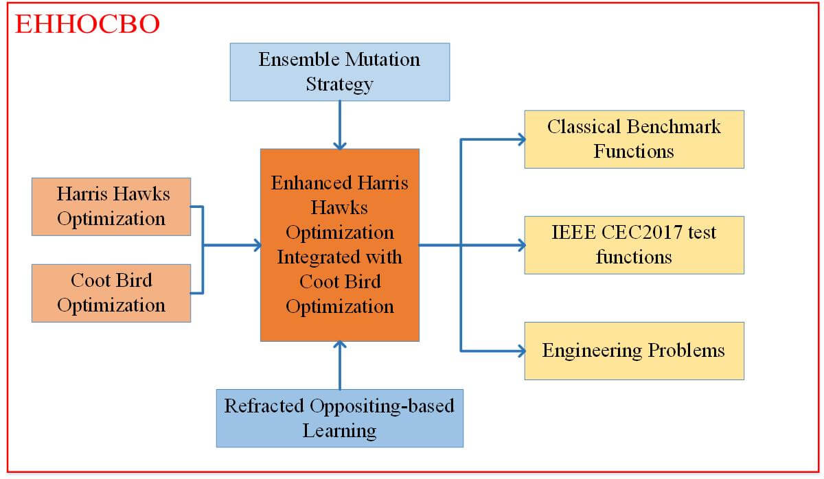
Harris Hawks Optimization (HHO) is a novel meta-heuristic algorithm that imitates the predation characteristics of Harris Hawk and combines Lévy flight to solve complex multidimensional problems. Nevertheless, the basic HHO algorithm still has certain limitations, including the tendency to fall into the local optima and poor convergence accuracy. Coot Bird Optimization (CBO) is another new swarm-based optimization algorithm. CBO originates from the regular and irregular motion of a bird called Coot on the water’s surface. Although the framework of CBO is slightly complicated, it has outstanding exploration potential and excellent capability to avoid falling into local optimal solutions. This paper proposes a novel enhanced hybrid algorithm based on the basic HHO and CBO named Enhanced Harris Hawks Optimization Integrated with Coot Bird Optimization (EHHOCBO). EHHOCBO can provide higher-quality solutions for numerical optimization problems. It first embeds the leadership mechanism of CBO into the population initialization process of HHO. This way can take full advantage of the valuable solution information to provide a good foundation for the global search of the hybrid algorithm. Secondly, the Ensemble Mutation Strategy (EMS) is introduced to generate the mutant candidate positions for consideration, further improving the hybrid algorithm’s exploration trend and population diversity. To further reduce the likelihood of falling into the local optima and speed up the convergence, Refracted Opposition-Based Learning (ROBL) is adopted to update the current optimal solution in the swarm. Using 23 classical benchmark functions and the IEEE CEC2017 test suite, the performance of the proposed EHHOCBO is comprehensively evaluated and compared with eight other basic meta-heuristic algorithms and six improved variants. Experimental results show that EHHOCBO can achieve better solution accuracy, faster convergence speed, and a more robust ability to jump out of local optima than other advanced optimizers in most test cases. Finally, EHHOCBO is applied to address four engineering design problems. Our findings indicate that the proposed method also provides satisfactory performance regarding the convergence accuracy of the optimal global solution.Graphic Abstract
Keywords
The optimization process refers to determining the best solution for a given problem. Optimization problems are widespread in the contemporary military, engineering, and management fields. Optimization methods have become an essential computational tool for technicians in different specialties [1–4]. With the evolution of human society and technology, more complex optimization problems are emerging. However, mathematical-programming optimization algorithms cannot effectively solve these problems, such as the Gradient Method and Newton’s Method. These conventional methods need help to locate the optimal global solution in large-scale, high-dimensional, and sub-optimal search domains [4–6]. To accomplish more powerful optimization tools, in recent decades many scholars have embarked on the research of meta-heuristic algorithms (MAs) [7]. MAs are a combination of stochastic algorithms and local search algorithms. The design of MAs is mainly inspired by a series of random phenomena in nature [8,9]. For MAs, they are concept-simple, require few parameter settings, and do not have any special requirements for the objective function. Consequently, MAs are not limited to specific problems and can be used in many applications [10,11]. MAs usually includes four categories [12–14]: evolutionary-based algorithms, physics-based algorithms, swarm-based algorithms (social behaviors of organisms in nature), and human-based algorithms. Some famous algorithms are Genetic Algorithm (GA) [15], Differential Evolution (DE) [16], Evolution Strategy (ES) [17], Simulated Annealing (SA) [18], Multi-Verse Optimizer (MVO) [19], Atom Search Optimization (ASO) [20], Arithmetic Optimization Algorithm (AOA) [21], Particle Swarm Optimization (PSO) [22], Sine Cosine Algorithm (SCA) [23], Sooty Tern Optimization Algorithm (STOA) [24], Chimp Optimization Algorithm (ChOA) [25], Aquila Optimizer (AO) [26], Dragonfly Algorithm (DA) [27], Butterfly Optimization Algorithm (BOA) [28], Slime Mould Algorithm (SMA) [29], Whale Optimization Algorithm (WOA) [30], Grey Wolf Optimizer (GWO) [31], Seagull Optimization Algorithm (SOA) [32], Gorilla Troops Optimizer (GTO) [33], Search Group Algorithm (SGA) [34], etc. Although hundreds of MAs have been proposed since the Artificial Intelligence (AI) age, the No Free Lunch (NFL) [35] theorem states that there is no single algorithm capable of tackling all optimization problems. Hence, further innovation in MAs is indispensable. At the same time, most MAs still need help with slow convergence, difficulty getting rid of local optimization, and imbalance between exploration and exploitation stages [36]. In addition to developing new MAs, several researchers try to boost the performance of existing algorithms by incorporating various search operators and achieving promising results. Nguyen et al. [13] proposed an improved Slime Mould Algorithm and applied it to control stepped hydropower plants. Debnath et al. [37] hybridized the Dragonfly Algorithm with Differential Evolution to better solve the problem of maximizing secondary user throughput in energy-harvesting cognitive radio networks. Ziyu et al. [38] proposed an improved Particle Swarm Optimization algorithm named TACPSO by introducing acceleration factors and random speeds. Li et al. [39] combined Differential Evolution and Hunger Games Search into a new DECEHGS algorithm, validated on the CEC2014 test suite, CEC2017 test suite, and four engineering problems. Jia et al. [40] constructed an improved Condor Search Algorithm based on the Lévy flight and simulated annealing mechanisms. All the above-improved variants are proven to outperform the basic algorithm to some extent, which indicates that it is feasible to enhance the performance of algorithms by introducing some additional search strategies.
The Harris Hawks Optimization (HHO) simulates the cooperative behavior and chasing style of Harris hawks in nature [41]. HHO is easy to implement with few parameters and performs well in solving many optimization problems. However, the basic HHO algorithm has several limitations, including the tendency to fall into the local optima and poor convergence accuracy. Its insufficient exploration phase causes this. Research on the improvement of HHO has been in full swing. For example, Fan et al. [42] proposed a quasi-reflective Harris Hawks Algorithm (QRHHO), enhancing the native algorithm’s exploration capability and convergence speed. Dokeroglu et al. [43] presented an island parallel HHO (IP-HHO) version of the algorithm for optimizing continuous multi-dimensional problems. Wang et al. [44] hybridized the exploration phase of Aquila Optimizer and the exploitation phase of Harris Hawks Optimization to preserve the powerful search abilities of each in both algorithms. They presented a novel improved optimizer, namely IHAOHHO. Another algorithm discussed in this paper is Coot Bird Optimization (CBO), proposed by Naruei et al. [45] in 2021. The CBO algorithm mimics four movement patterns of coot birds on the water surface, including random movement, chain movement, location adjustment according to the group leaders, and leader movement. In this algorithm, the Coot leaders continuously lead the population toward the goal. The leaders sometimes have to leave their current positions to find better target areas, which gives the algorithm have strong global ability to explore different parts of the search space. But the overall framework of CBO is relatively complex compared to other algorithms, and its exploitation stage needs to be revised, often leading to premature convergence. Considering this, mixing HHO and CBO can compensate for the lack of HHO exploration capability and thus improve its global search performance. The hybrid algorithm can effectively use the solution information in the search space to maintain population diversity later in the search. Currently, some improved variants of the CBO-based algorithm have achieved promising performance. Huang et al. [46] developed a COOTCLCO algorithm that provided satisfactory solutions for solving the uneven distribution and low coverage problems of randomly deployed Wireless Sensor Network (WSN) nodes.
Motivated by the NFL theory and fully considering the characteristics of the basic HHO and CBO algorithms: HHO has good exploitation properties, but its exploration stage is insufficient, and conversely, CBO owns excellent exploration capability benefiting from the leader mechanism, but the algorithm itself is complex and lacks exploitation ability. Therefore, this paper attempts to combine the basic HHO and CBO algorithms by taking advantage of each and proposes a novel hybrid meta-heuristic algorithm with better all-around search performance for global optimization, called EHHOCBO. First, integrate the leadership mechanism of CBO into the population initialization stage of HHO. In the leader movement, the optimal individual guides the whole population to explore all regions of the search space as much as possible in a circular envelope so that the algorithm has good randomness and rich population diversity. It can make up for the lack of helpful information exchange between the optimal individual and other individuals in the swarm, thus laying a good foundation for the global search of HHO. Then, during the iterative computation, Ensemble Mutation Strategy (EMS) [47] is introduced to generate the variant candidate positions of the current individual further to enhance the algorithm exploration capability and convergence accuracy. Moreover, to extend the search range and avoid the algorithm from falling into the local optima in the later search phase, Refracted Opposition-Based Learning (ROBL) [48] is used to evaluate the fitness value of the inverse position of the current optimal solution and perform the update. To assess the performance of the proposed EHHOCBO, we used 23 classical benchmark functions and the IEEE CEC2017 test suite for testing and applied the proposed algorithm to address four engineering problems. Experimental results demonstrate that EHHOCBO performs better than competitors concerning solution accuracy, convergence speed, stability, and local optima avoidance.
This paper is organized as follows: Section 2 briefly introduces the basic HHO and CBO algorithm and two improved search strategies. In Section 3, the proposed hybrid EHHOCBO optimizer is described in detail. In Section 4, we evaluate the performance of EHHOCBO through a series of simulation experiments and analyze the results obtained. Based on this, the proposed method addresses four real-world engineering design problems to highlight its practicality in Section 5. Finally, a conclusion of this paper is provided in Section 6.
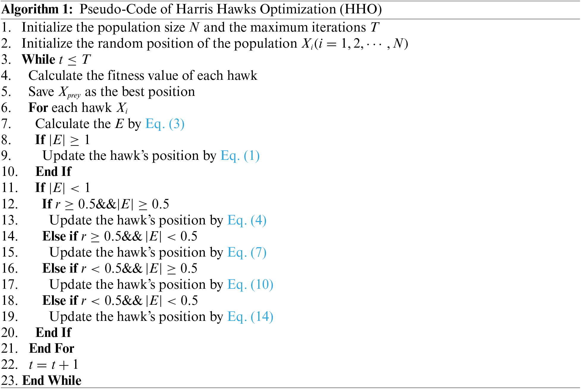
2.1 Harris Hawks Optimization (HHO)
Harris Hawks Optimization (HHO) was proposed by Heidari et al. [41] in 2019, which mimics the predatory behavior of the Harris Hawk, a species of raptor living in southern Arizona, U.S.A. The HHO algorithm consists of three main components: the exploration phase, the exploitation phase, and the transition from exploration to exploitation. Fig. 1 shows the different search processes of the basic HHO algorithm.
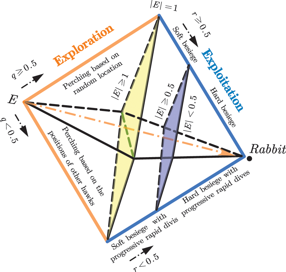
Figure 1: Different phases of HHO
During this phase, the Harris hawks randomly perch in certain places. They detect the prey with keen vision and then choose between two strategies with the same probability of undertaking hunting activities. The formula for the position update of Harris hawk in this phase is as follows.
where
where
2.1.2 Transition from Exploration to Exploitation
In the HHO algorithm, the prey’s escape energy
where
Four possible strategies exist in the exploitation phase, including soft besiege, hard besiege, soft besiege with progressive rapid dives, and hard besiege with progressive rapid dives, to simulate the attack process of Harris hawk on its prey.
• Soft Besiege
The soft besiege is performed when
where
• Hard Besiege
The hawk will take a hard besiege when
• Soft Besiege with Progressive Rapid Dives
When
where
where
• Hard Besiege with Progressive Rapid Dives
When
where
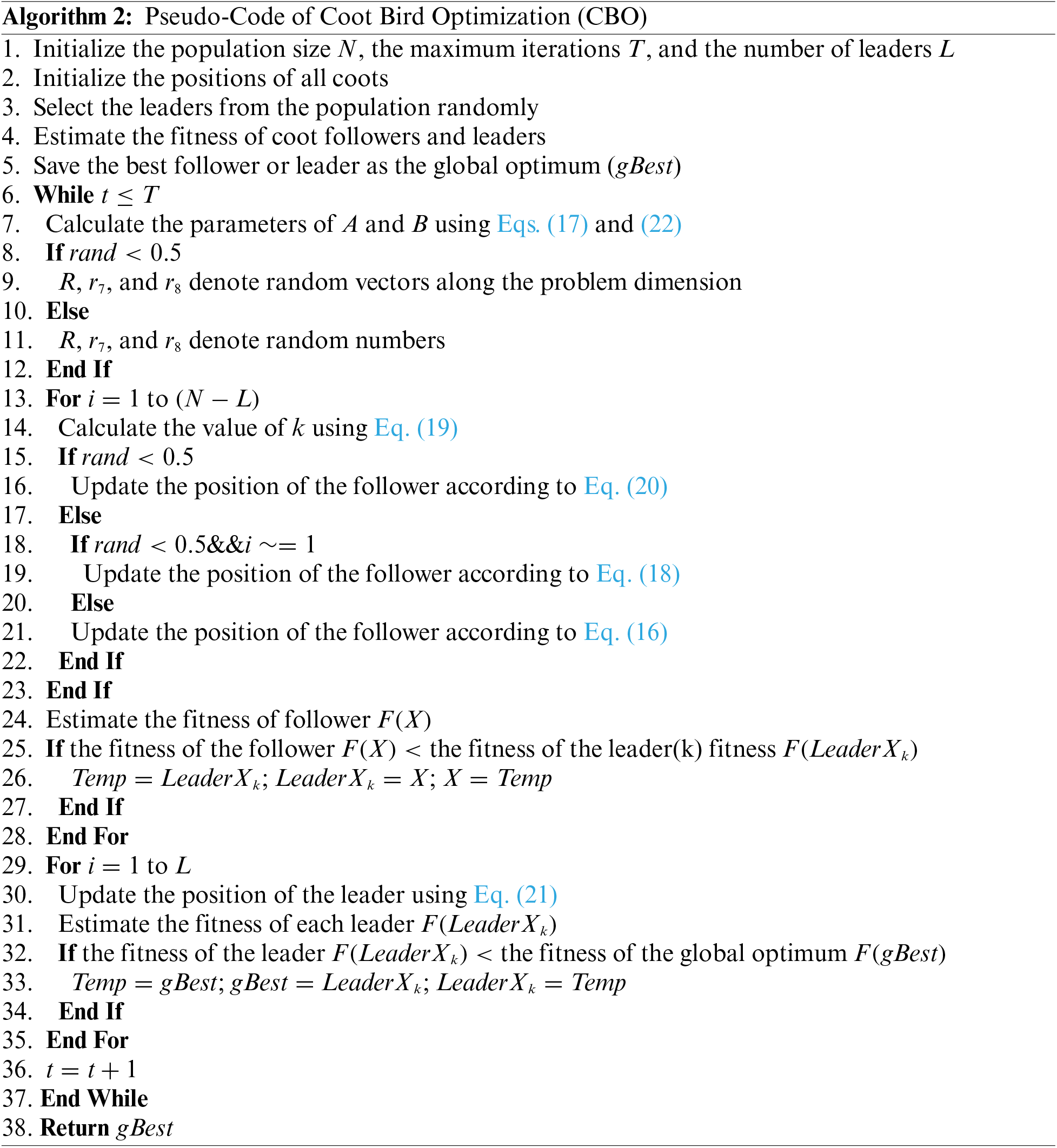
2.2 Coot Bird Optimization(CBO)
Coot Bird Optimization (CBO) is a bio-inspired, population-based, and gradient-free optimization technique developed by Naruei et al. [45] in 2021, which mimics the collective behaviors of American Coots (a small water bird) on the water surface. In the CBO, there are four different irregular and regular movements implemented: (1) Random movement, (2) Chain movement, (3) Adjusting the position based on the group leaders, and (4) Leader movement. The mathematical model of the algorithm is presented below.
Usually, the Coots live in a group and make a chain structure to move toward the target area (food). In front of the group are a few coots, also known as group leaders, who guide the direction and take charge of the whole flock. Therefore, according to the habits of Coots, the initial population is divided into two parts: the leader Coots and the follower Coots. If
In this stage, the random position
where
where
where
In the Salp Swarm Algorithm (SSA), the average position of two individuals is used to perform chain movements. The same approach is employed in CBO. The new position of the Coot follower is calculated as follows:
where
2.2.3 Adjust the Position Based on the Group Leaders
Generally, the whole group is led by some of the group leaders in the front, and all the remaining coot followers need to adjust their position based on the leaders and move towards them. However, a severe issue that must be addressed is that each Coot should update its position according to which leader. Eq. (19) is designed to select the leader as follows:
where
The next position of the Coot follower based on the selected leader
where
The group must be oriented towards the optimal area, so in some instances, the leaders have to leave the current optimal position to search for a better one. The formula for updating the leader position is given as follows:
In Eq. (21),
where
2.3 Ensemble Mutation Strategy (EMS)
The set variation strategy is a new improvement mechanism proposed by Zheng et al. [8,47], which can generate diverse individuals to improve the global search capability of the hybrid algorithm. The mathematical formula of EMS is as follows:
where
After the mutant candidate positions
where
2.4 Refracted Opposition-Based Learning
Refracted Opposition-based Learning [48] is an improved variant of Opposition-based Learning (OBL) [49]. ROBL introduces the principle of refraction of light to generate dynamic inverse solutions based on OBL, which solves the limitation that OBL can easily fall into local optimum in later iterations. Currently, ROBL has been used to effectively improve the optimization performance of the Grey Wolf Optimizer (GWO) [31]. The schematic diagram of ROBL is shown in Fig. 2, and its mathematical model is formulated as follows:
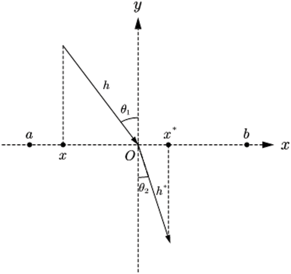
Figure 2: Refracted opposition-based learning
where
where
3 The Proposed EHHOCBO Algorithm
This section integrates the basic HHO and CBO algorithms into a new swarm intelligence algorithm called EHHOCBO. EHHOCBO takes HHO as the core framework and is hybridized with the powerful exploratory leadership mechanism of hybrid CBO. In addition, ensemble mutation strategy (EMS) and refracted opposition-based learning (ROBL) are introduced into the preliminary hybrid algorithm to enhance its search performance further.
According to Section 2, the basic HHO algorithm consists of three main steps: the exploration phase, the transition from exploration to exploitation, and the exploitation phase. In the exploration phase, Harris hawk detects prey in the search space with two equal probabilities. After detecting prey, the hawk transitions between global and local search based on the decay of prey energy. In the exploitation phase, the energy of the prey and the probability of the prey escaping determine the four different predation methods that the Harris hawk will adopt, namely soft besiege, hard besiege, soft besiege with progressive rapid dives, and soft besiege with progressive rapid dives. When the prey escapes successfully, the Lévy flight is introduced into the algorithm to ensure that the algorithm can jump out of the local optima. In the basic algorithm, the Lévy flight is only used when the position has a better fitness value, which leads to the algorithm being unable to jump out of the local optimum well. The low population diversity and simple search method in the exploration phase weaken the global search capability of HHO. This leads to a longer time to obtain the optimal global solution and increases the possibility of getting stuck in local optima. These can be improved to explore better and exploit the HHO algorithm [50]. For the CBO algorithm, the population is divided into a few randomly chosen Coot leaders and Coot followers. The leaders can make full use of the information in the search space and have a strong tendency to explore, thus effectively leading the followers to the target area. CBO mainly consists of individual random movement, chain movement, and optimal individual-guided movement. The CBO algorithm will choose a random position in the search space as a reference, which is also a an excellent way to help the algorithm jump out of the local optimum. Chain movement allows the algorithm to quickly improve the accuracy of the algorithm when the population is concentrated. In the leader movement of the optimal individual, the position of the follower will change with the position of the corresponding leader. This allows the leader to lead the followers closer and closer to the optimal region. In this paper, the optimal individual movement mechanism of CBO is integrated into the population initialization of HHO to take full advantage of the strengths of both algorithms. In the CBO optimal individual-led movement,
where
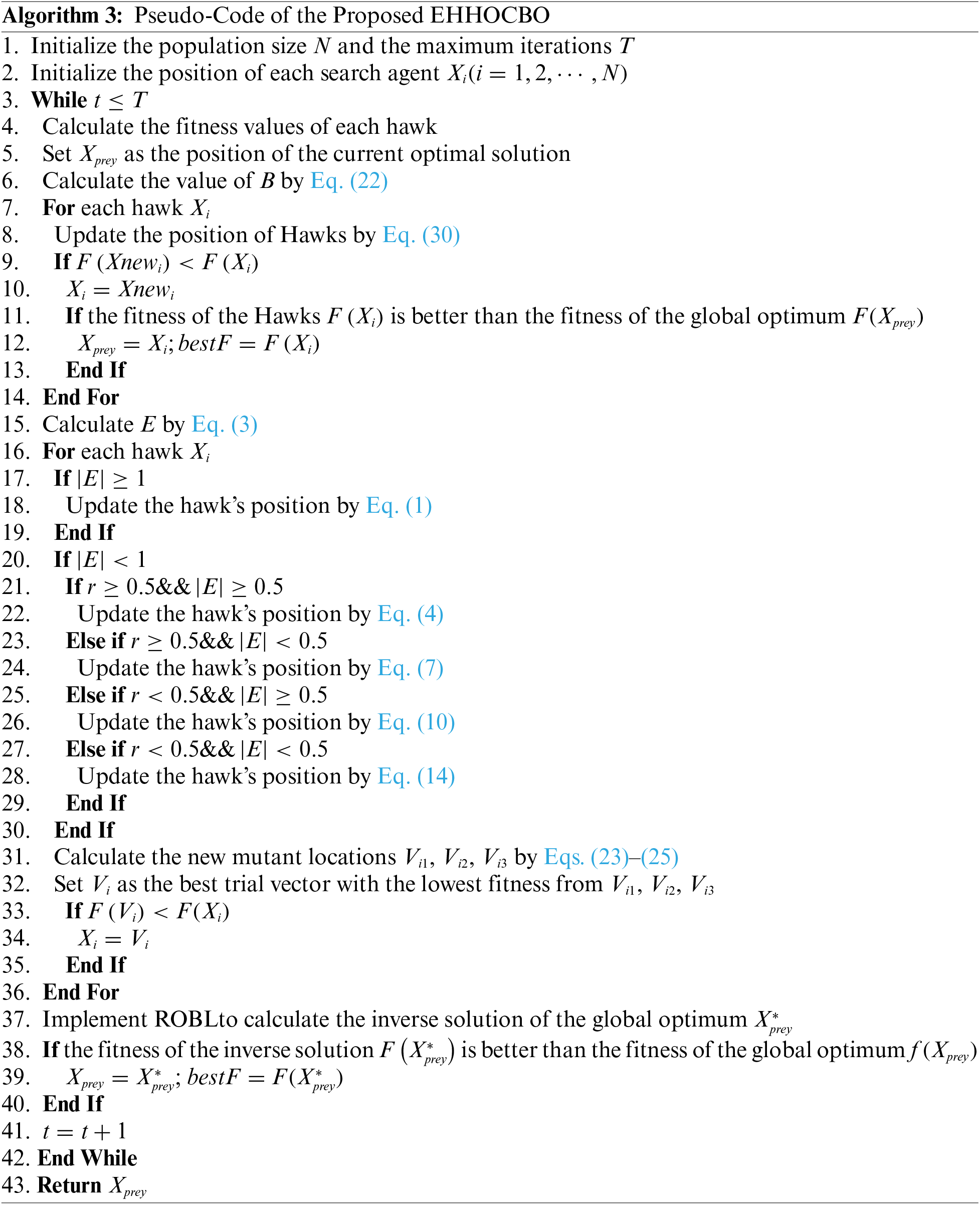
Secondly, although the basic HHO algorithm introduces the Lévy flight to ensure that it can jump out of the local optimum, it still has limitations that can cause the algorithm to fall into a local optimum in later iterations. The EMS has multiple mutation operators, which can generate three differentcandidate positions according to Eqs. (23)–(25). Then, the mutant positions with the lowest fitness is selected for comparison with the fitness of the original positions. The position with the highest fitness is selected as the new position. In this way, the global search ability of the algorithm can be improved. At the end of the algorithm, ROBL is integrated into the HHO. The inverse solution of the current optimum is generated by Eq. (27). This can expand the search range, improve the convergence speed, and reduce the possibility of falling into the local optima. The introduction of EMS and ROBL strategies makes up for the shortcomings of the basic HHO algorithm in the exploitation stage. The flowchart and pseudo-code of the proposed EHHOCBO are shown in Fig. 3 and Algorithm 3, respectively.
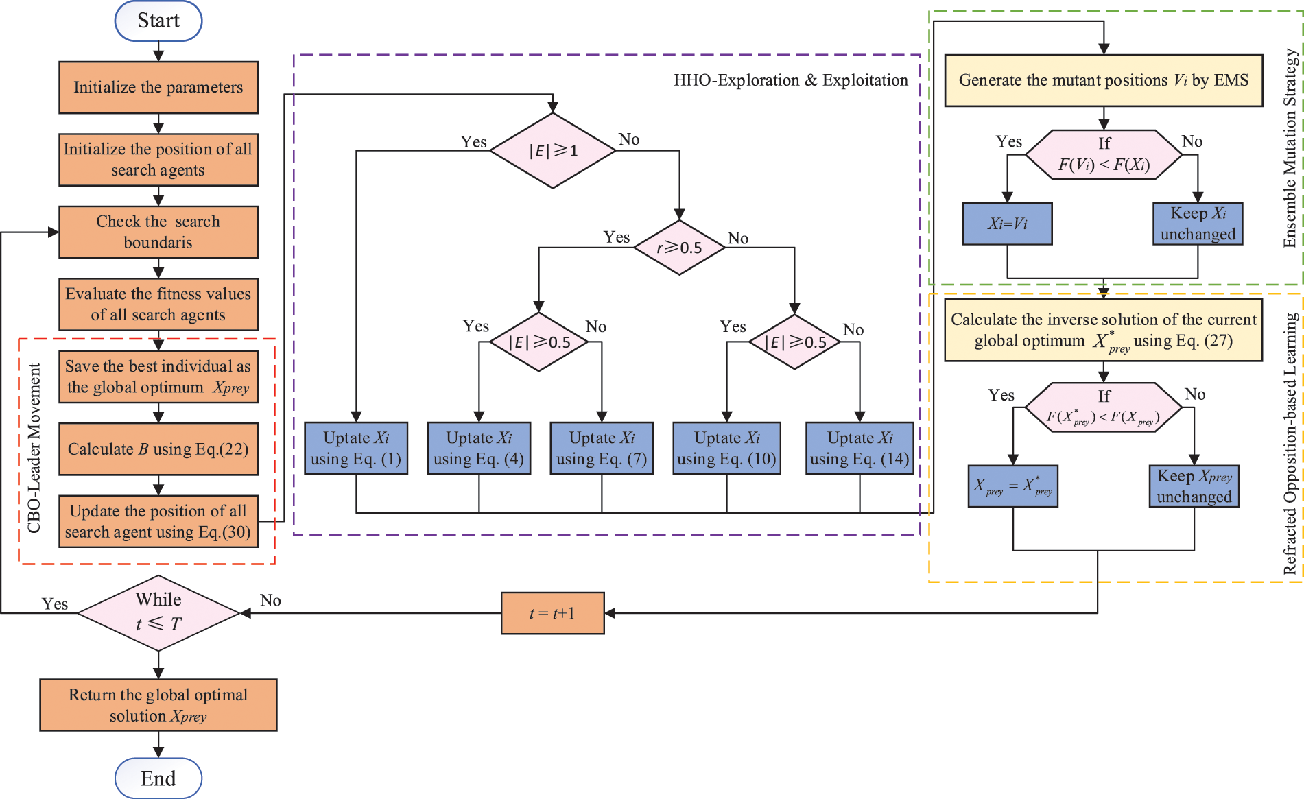
Figure 3: Flow chart of the proposed EHHOCBO algorithm
4 Experimental Results and Discussions
In this section, the effectiveness and feasibility of the proposed EHHOCBO is validated on two sets of optimization problems. Firstly, the performance of the algorithm in solving simple numerical problems is verified by 23 classical benchmark functions [51]. The algorithm’s performance in solving complex numerical optimization problems is evaluated using the IEEE CEC2017 benchmark functions [52]. All experiments were conducted on Windows 10 operating system with a computer hardware configuration of Intel(R) Core(TM) i5-7300HQ CPU@2.50 GHz and 8 GB RAM, and the tool used was MATLAB2020a software.
4.1 Experiment 1: Classical Benchmark Functions
In this section, 23 classical benchmark functions are used to evaluate the performance of EHHOCBO. The functions F1–F7 are unimodal and are used to assess the development capability of the algorithm. F8–F13 are multimodal, which are used to test the exploration capability of the algorithm and its ability to escape from local optimum solutions. F14–F23 are fixed-dimension multimodalities, a combination of unimodal and multimodal, used to evaluate the stability of an algorithm between exploration and exploitation [51]. The population size and maximum iterations for all algorithms were set to 30 and 500, respectively, for a fair comparison. In the proposed EHHOCBO, we set the refraction index
• Harris Hawks Optimization (HHO) [41]
• Coot Bird Optimization(CBO) [45]
• Arithmetic Optimization Algorithm (AOA) [21]
• Whale Optimization Algorithm (WOA) [30]
• Grey Wolf Optimizer (GWO) [31]
• Particle Swarm Optimization (PSO) [22]
• Sooty Tern Optimization Algorithm (STOA) [24]
• Chimp Optimization Algorithm (ChOA) [25]


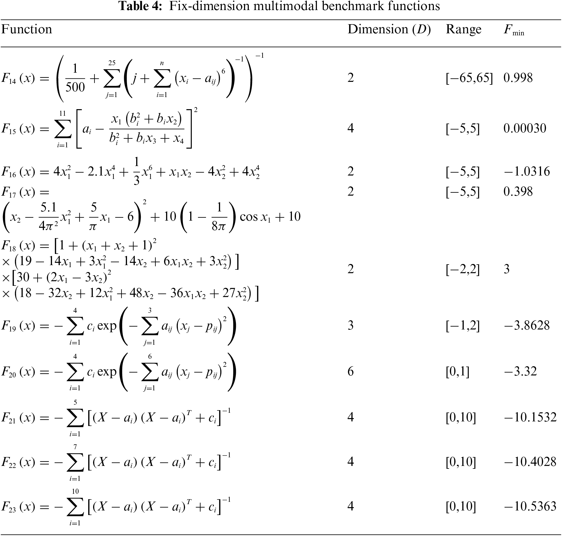
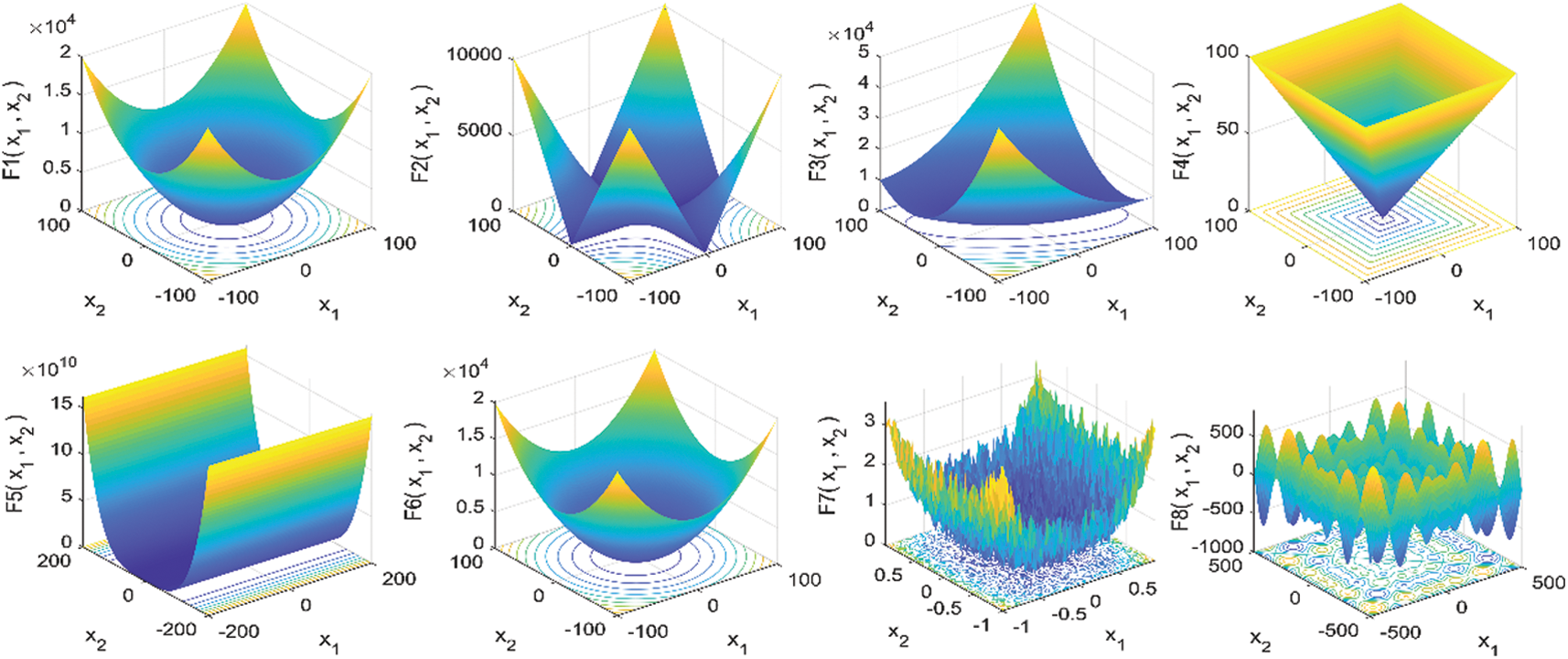
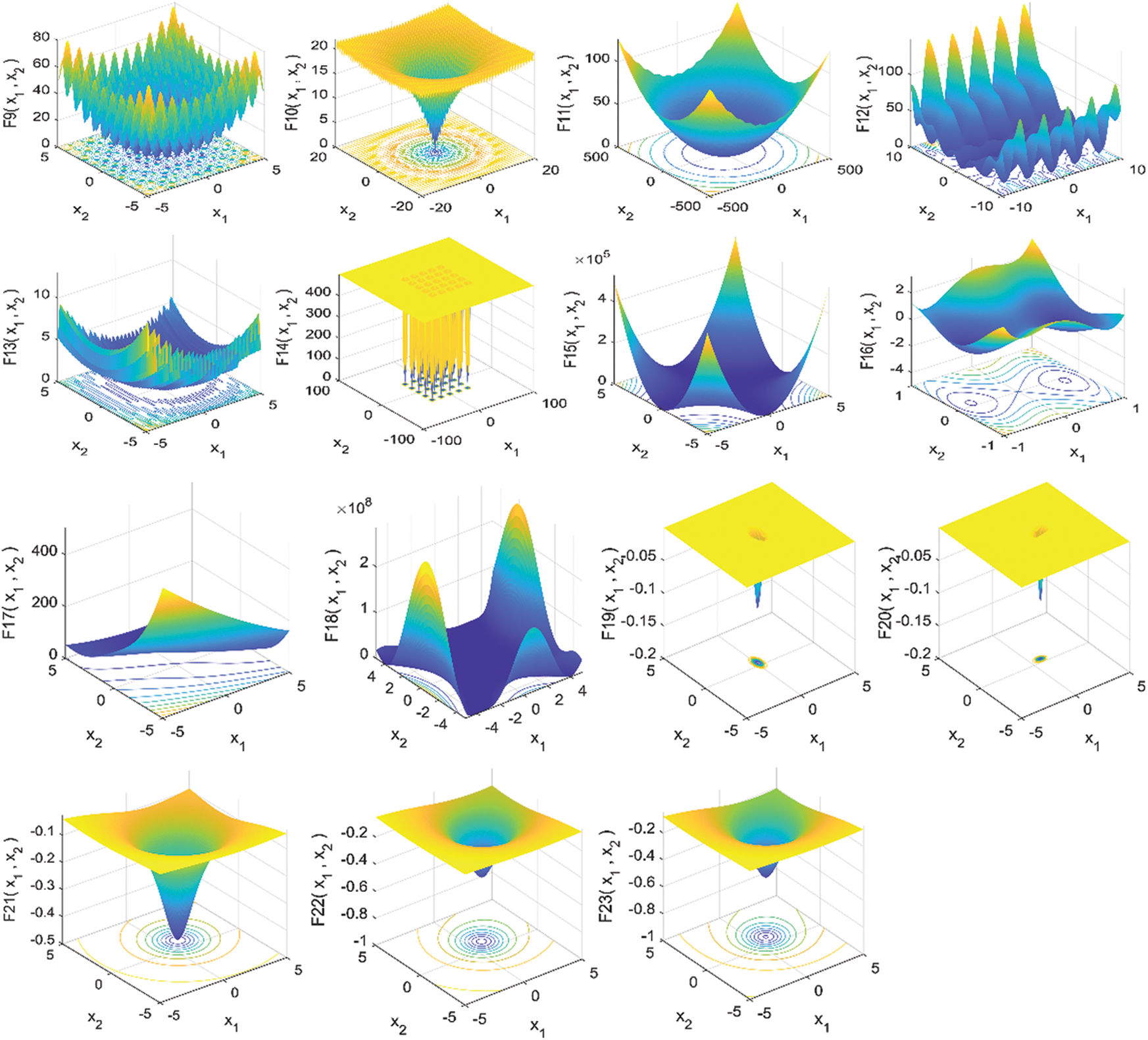
Figure 4: 3D view of the search space for 23 benchmark functions
In order to evaluate the performance of the algorithm more intuitively, this paper introduces the Mean fitness (Mean) and Standard deviation (Std) evaluation indicators. The difference between the mean fitness and the target value represents the convergence accuracy of the algorithm. The standard deviation evaluates the degree of fluctuation of the experimental results. The size of the Std depends on how stable the algorithm is. The following formula calculates them:
where
4.1.1 Effectiveness of the Introduced Strategy
This paper first integrates the original HHO and CBO algorithms into a new intelligent algorithm named EHHOCBO. The algorithm takes HHO as the core framework, introduces the strong exploratory leadership mechanism of CBO, and then improves the algorithm with EMS and ROBL strategies. To investigate the impact of each improved component on the algorithm, this paper designs a comparison experiment between EHHOCBO and three other derived algorithms (EHHOCBO1, EHHOCBO2, EHHOCBO3). EHHOCBO1 only introduced the leadership mechanism of CBO into the algorithm. EHHOCBO2 introduces the leadership mechanism of the CBO algorithm and the EMS strategy into the algorithm. EHHOCBO3 introduces the leadership mechanism of the CBO algorithm and ROBL strategy. The performance of these four algorithms is tested using 23 standard test functions under the same parameter settings, and the sizes of Mean and Std are listed in Table 5.
The experimental results show that in comparing between EHHOCBO and the remaining three derived algorithms, EHHOCBO has better simulation results on the test functions F1–F23. This verifies the effectiveness of the improved method in this paper. The theoretical minimum of the test functions was achieved for the test functions F1–F4, F8, F9, F11, F14, F16–F19, and F23. The remaining three derived algorithms also reached theoretical minima in some test functions, but the overall performance shows a different advantage than the EHHOCBO algorithm. In terms of standard deviation, the simulation results of EHHOCBO also obtained better results. This shows that EHHOCBO has strong stability in solving all test functions. The results show that the improvements in this paper significantly improve the performance of the original HHO algorithm. The improved method in this paper enables the EHHOCBO algorithm to obtain strong exploration and utilization capabilities, laying a foundation for the ability to provide high-quality solutions. After validation, EHHOCBO was selected as the final version for further comparison and discussion.
4.1.2 Comparison between EHHOCBO and Other Optimization Algorithms
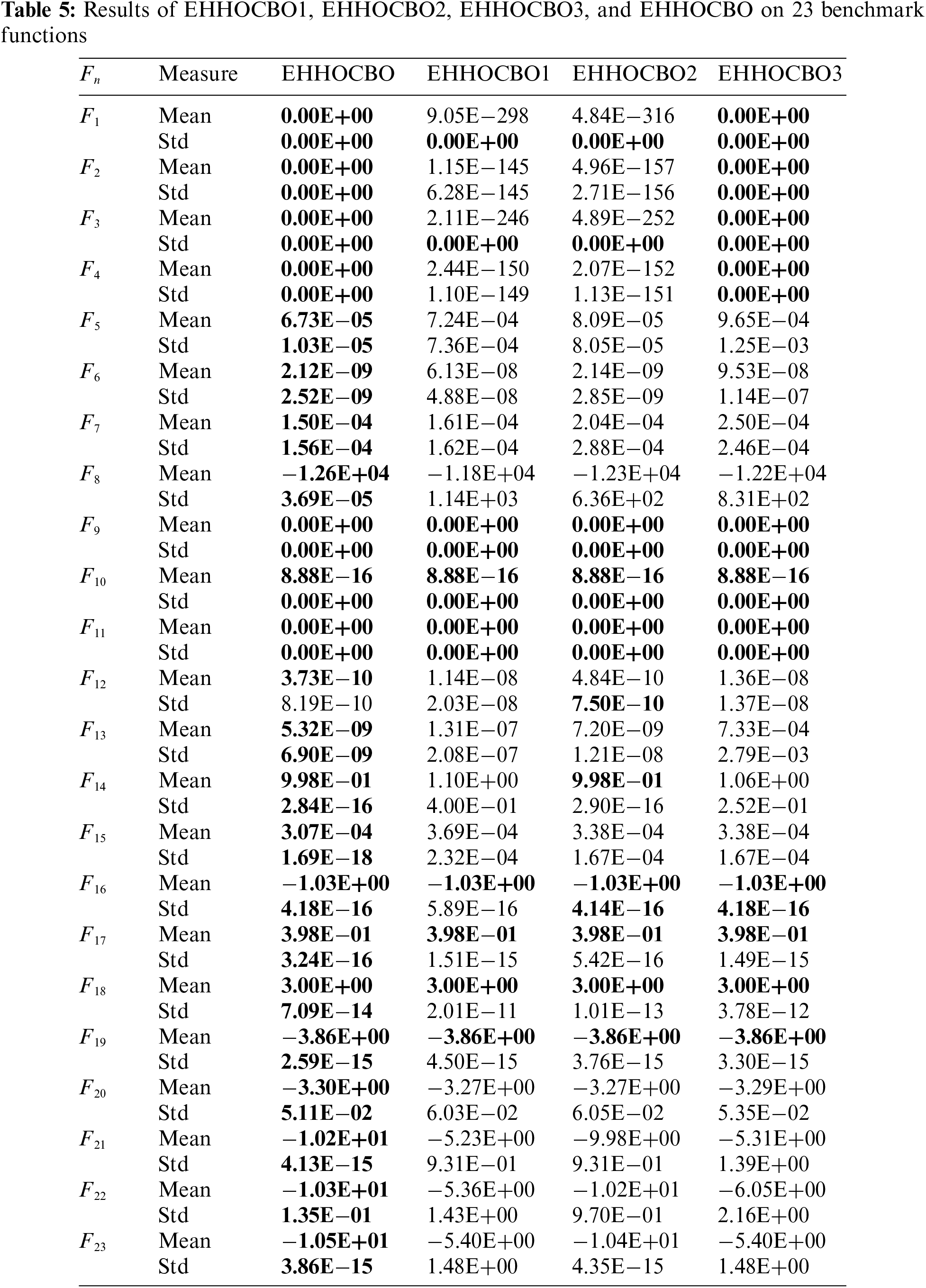
This section evaluates the proposed algorithm’s exploration and development capabilities using standard test functions. The above eight well-known algorithms are compared mainly from numerical analysis, box plot, convergence curve, and Wilcoxon test. After 30 independent runs of the experiment. The Mean and Std of the obtained results are recorded in Table 6 below.
The proposed EHHOCBO experiment showed better mean fitness and standard deviation. The EHHOCBO has an overwhelming advantage in solving the unimodal test function problem. In the test functions F1–F4, the EHHOCBO can acquire the theoretically global optimal solution compared with the original HHO algorithm and CBO algorithm. In the multi-dimensional test functions F8–F13, the EHHOCBO algorithm achieves better simulation results than the other algorithms. It is worth mentioning that in functions F9 and F11, EHHOCBO obtains the ideal optimal value. The experimental results of the unimodal and multimodal functions fully demonstrate that the EHHOCBO has a better exploitation and exploration capability and a higher possibility of jumping out of the local optimum solution. This shows that the introduced improvement strategy greatly improves the relationship between exploration and exploitation in the HHO algorithm. The EHHOCBO integrates the leadership mechanism of the CBO algorithm into the population initialization of the HHO algorithm. In this way, the stable exploration and development capabilities of the two algorithms are extracted so that the algorithm can easily jump out of the local optimum. For the fixed-dimension benchmark functions F14–F23, the EHHOCBO algorithm obtains better solutions and smaller deviations. Especially in the functions F14, F16–F19, EHHOCBO obtained the theoretically optimal Mean and Std. The smaller Std indicates that the EHHOCBO has higher stability, which can ensure that the algorithm can obtain more accurate results in the application process. The fixed dimension test function results show that the proposed EHHOCBO has good stability between exploration and exploitation due to the introduction of the EMS improvement strategy.
Boxplots are drawn in this paper to visualize the distribution of the data. It can well describe the consistency between data. Fig. 5 depicts the boxplot of EHHOCBO against eight other comparison algorithms over 15 representative benchmark functions. In this figure, serial numbers 1–9 correspond to the algorithms in the table in order, specifically 1-GWO, 2-WOA, 3-PSO, 4-AOA, 5-HHO, 6-ChOA, 7-STOA, 8-CBO, and 9-EHHOCBO. As can be seen from Fig. 5, the EHHOCBO algorithm has better consistency than other original algorithms. No outliers were generated during the iteration. The obtained median, maximum and minimum values are more concentrated than other comparison algorithms and only slightly worse than the HHO algorithm in function F6. The above confirms the high stability of EHHOCBO.
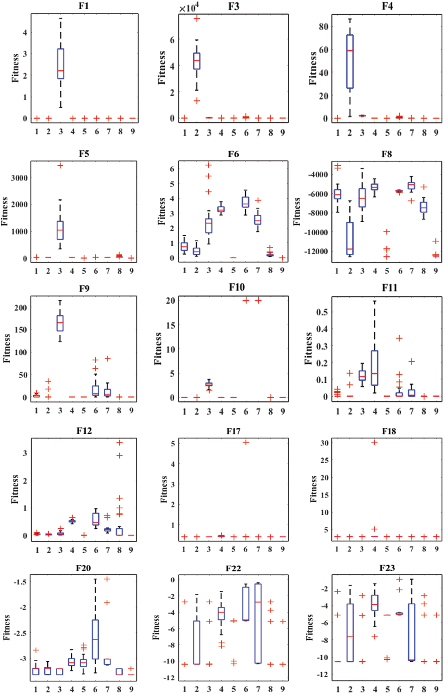
Figure 5: Boxplot analysis on 23 benchmark functions
In order to study the convergence behavior of the EHHOCBO algorithm, this paper compares the convergence curve of the EHHOCBO algorithm with the convergence curves of the other eight comparison algorithms on some representative test functions. The results are shown in Fig. 6. According to the convergence curve graph, we can see that the EHHOCBO algorithm has a better convergence performance. In the test functions F1, F3, and F4, the EHHOCBO algorithm can quickly converge to the global optimum, and its convergence curve shows the fastest decay trend. At the same time, other algorithms have obvious lag and slow convergence speed. This is because the algorithm introduces an improved strategy so that the algorithm have better randomness and population diversity. Among the test functions F5 and F6, the convergence of the EHHOCBO algorithm is also the best, and its convergence curve is consistent with that of HHO at the beginning of the iteration. But in the later stage, the convergence trend of HHO could be clearer, and the EHHOCBO algorithm still maintains good convergence until the end. This shows that the introduction of the improved strategy effectively reduces the possibility of the algorithm falling into the local optimum. In the multi-dimensional test functions F8–F12, the EHHOCBO algorithm also maintains good convergence. In test functions F9–F11, EHHOCBO converges to the optimal global solution only after several iterations. In F8, the convergence of EHHOCBO is slightly worse than that of HHO in the early stage. But in the later iterations, the HHO algorithm gradually falls into the local optimum, while the EHHOCBO algorithm still maintains good convergence performance. In F10–F12, although the EHHOCBO algorithm does not reach the theoretical optimum, its convergence performance and final accuracy are the best among all algorithms. The EHHOCBO algorithm also shows strong performance in solving fixed-dimensional testing problems. EHHOCBO converges rapidly in the early stages of testing functions F17, F18, F20, F22, and F23. And make a quick transitions between exploration and exploitation. Finally, the optimal value was determined. The convergence accuracy and operational efficiency of the EHHOCBO algorithm are also improved to some extent compared to HHO and CBO.
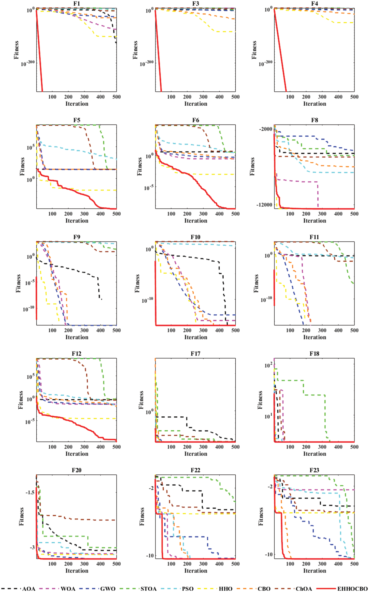
Figure 6: Convergence curves of different algorithms on fifteen benchmark functions
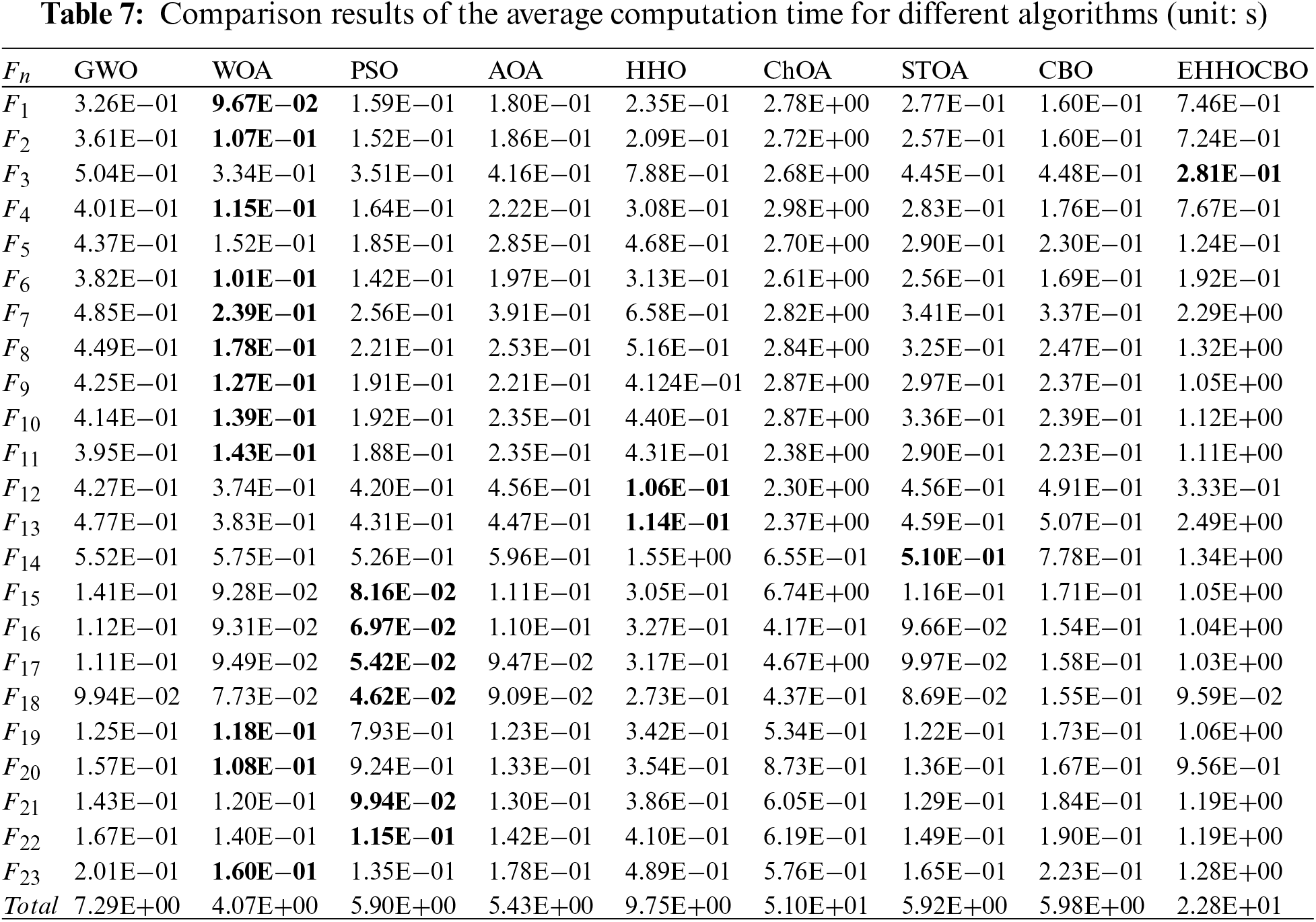
Table 7 reports the average computation time for each algorithm. The total running time for each algorithm is calculated and ranked as follows: ChOA(51 s) > EHHOCBO(22.8 s) > HHO(9.75 s) > GWO(7.29 s) > CBO(5.98 s) > STOA(5.92 s) > PSO(5.90 s) > AOA(5.43 s) > WOA(4.07 s). Table 7 shows that the EHHOCBO algorithm takes more time than the original HHO algorithm. The main reason is that the improved approach adds steps and extra time to the HHO algorithm. Overall, our proposed algorithm is acceptable due to the performance improvements.
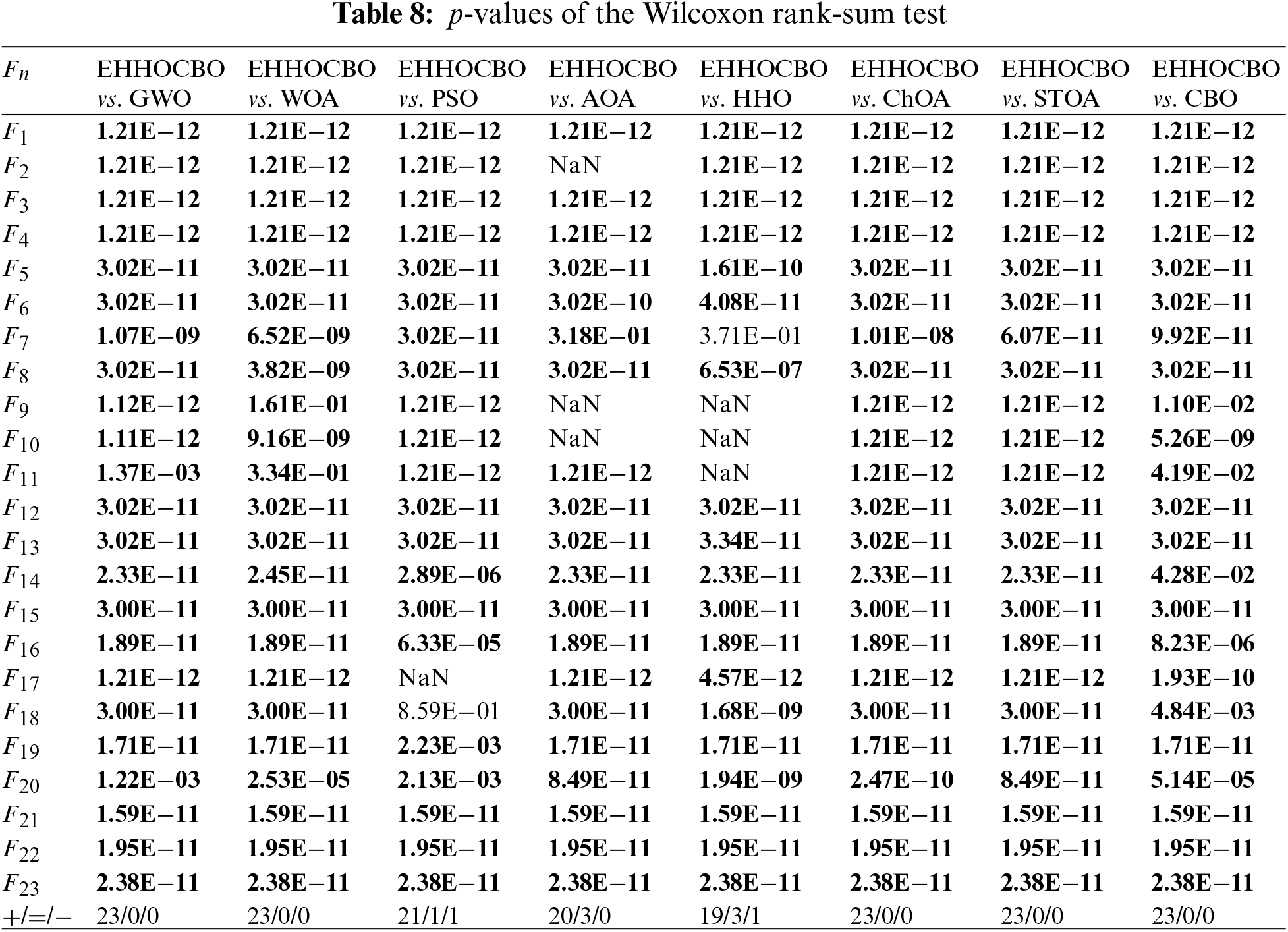
To better evaluate the correlation, the Wilcoxon rank sum test was designed, and the significance level was set at 0.05 [53]. The p-values are recorded in Table 8. In the table, the parts where EHHOCBO performs better are highlighted in bold. NaN indicates the same performance as the comparison algorithm. The rest is the part where EHHOCBO has poor performance. As can be seen from Table 8, EHHOCBO performs worse than some algorithms only on individual functions. EHHOCBO performs slightly worse than the PSO algorithm on F18 and slightly worse than the HHO algorithm on F7. In other cases, EHHOCBO achieved the same or better results. Based on statistical theory, EHHOCBO has better performance.
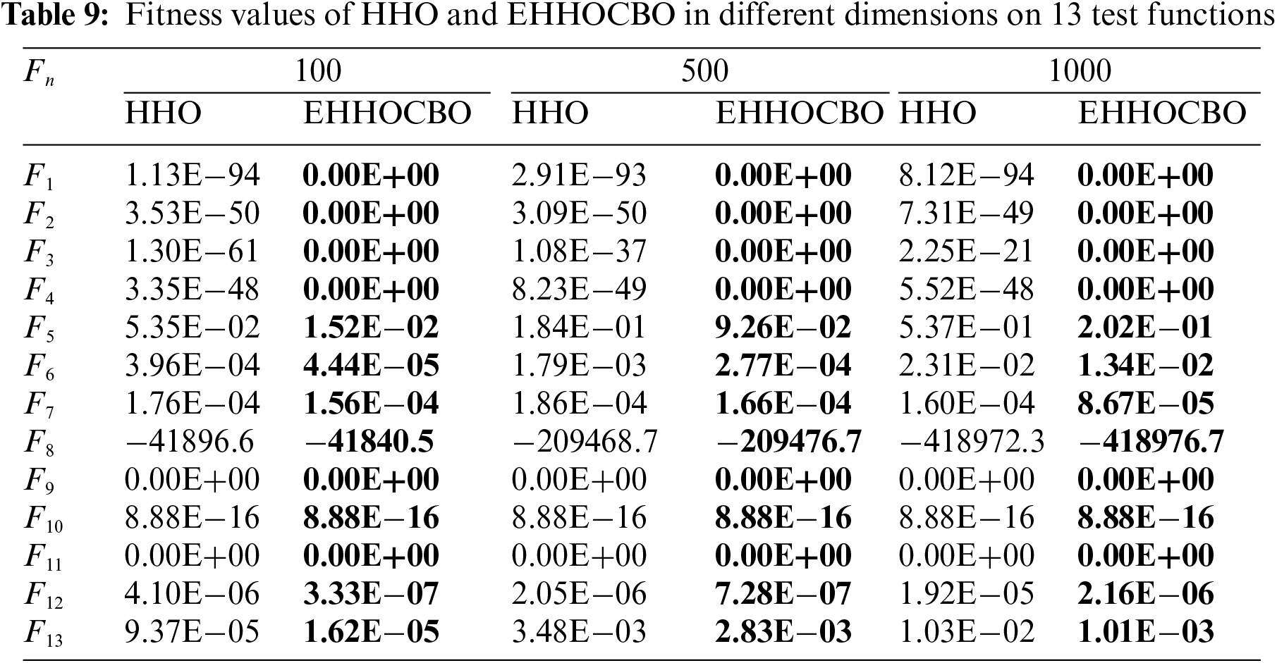
In addition, the performance of some optimization algorithms gradually deteriorates as the dimension of the problem expands. In this paper, EHHOCBO and HHO algorithms are simulated in different dimensions to evaluate the impact of scalability on the EHHOCBO algorithm. The experimental tools are F1–F13 of the standard test functions, and the results are recorded in Table 9. The experimental results show that the simulation accuracy of both the original HHO and EHHOCBO decreases with the increase in the number of iterations. However, the simulation results of EHHOCBO are consistently more accurate than HHO. The accuracy of EHHOCBO will remain relatively high and will always be kept in a relatively precise state. It is worth mentioning that EHHOCBO reaches the global optimal solution in F1–F4, F9, and F11. In conclusion, the EHHOCBO algorithm also performs well in solving high-dimensional problems.
4.2 Experiment 2: IEEE CEC2017 Test Functions
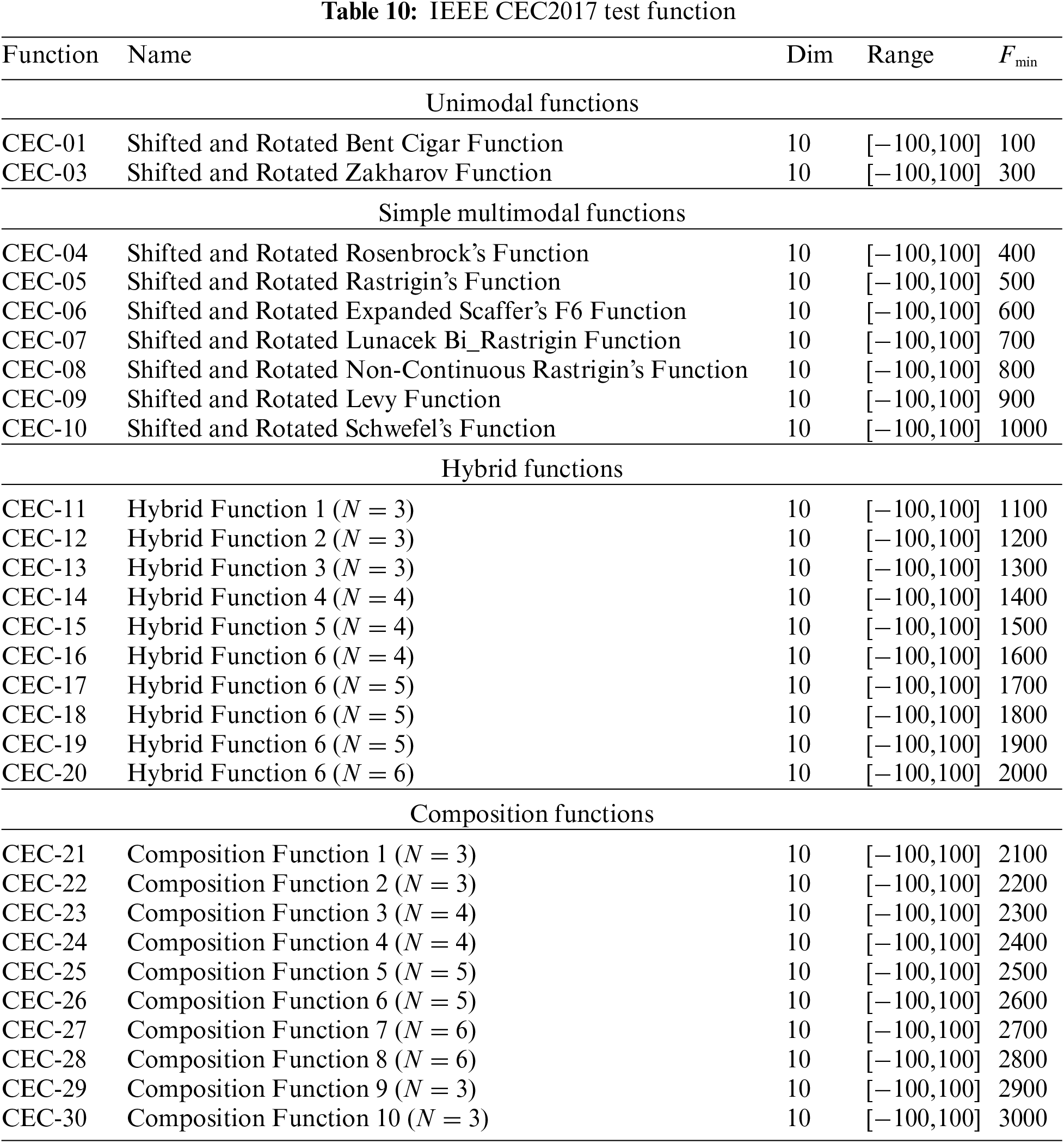
The benchmark function test proves that EHHOCBO performs well in solving simple problems, but is insufficient to prove its superior performance. To further exploit its performance, this paper applies the EHHOCBO algorithm to solve 29 test functions in IEEE CEC2017 [50,51] to evaluate its performance in solving complex numerical problems. In this section, comparative experiments are conducted between EHHOCBO and six well-known hybrid algorithms based on IEEE CEC2017 test functions. The six algorithms are the Differential Squirrel Search Algorithm (DSSA) [54], Equilibrium Slime Mould Algorithm (ESMA) [55], Grey Wolf Optimizer Based on Aquila Exploration Method (AGWO) [56], Teaching-Learning-Based Optimization Algorithm with Reinforcement Learning Strategy (RLTLBO) [57], Leader Harris Hawks optimization (LHHO) [58] and Hybrid Sine-Cosine Harris Hawks Optimization (SCHHO) [59]. IEEE CEC2017 test functions include 29 functions, which are widely used for performance testing and evaluation of intelligent bee swarm algorithms. Among them, CEC-1 and CEC-3 are single-peaked functions, F4–F10 are simple multi-peaked functions, CEC-11 to CEC-20 are hybrid functions, and CEC-21 to CEC-30 are combined functions. Table 10 lists these functions’ names, dimensions, target values, and search ranges. The proposed EHHOCBO algorithm was run independently of the other comparison algorithms 30 times. The population size and maximum iterations were set to 30 and 500. The mean and standard deviation obtained were recorded in Table 11.
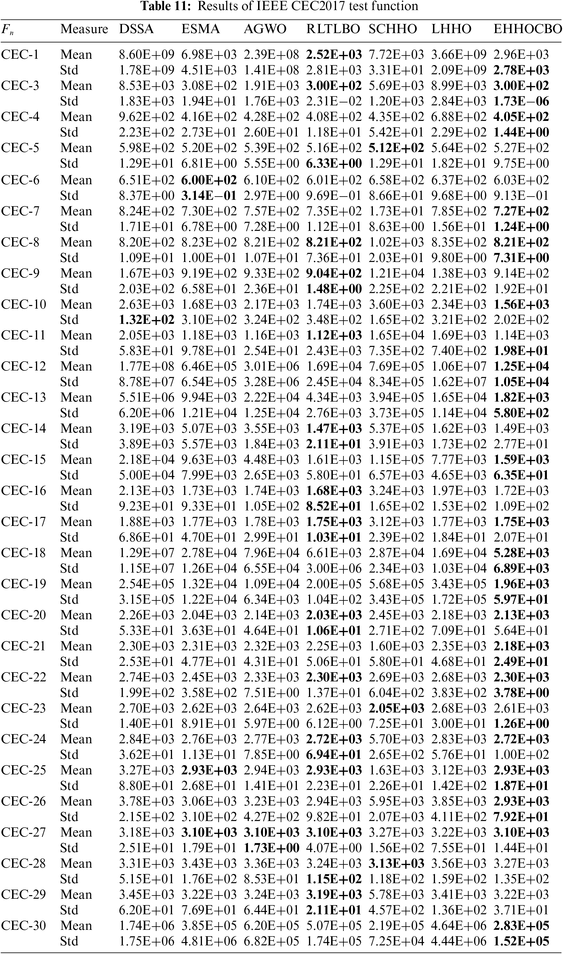
The results show that the performance of the EHHOCBO algorithm is significantly better than that of DSSA, ESMA, AGWO, LHHO, and SCHHO algorithms and is comparable to the performance of the RLTLBO algorithm. For unimodal functions CEC-1 and CEC-3, EHHOCBO gives better simulation results, but in CEC-1, the standard deviation of the algorithm is slightly worse than RLTLBO. For multimodal functions, EHHOCBO achieves the best standard deviation in the test functions CEC-4, CEC-7, CEC8, and CEC-10, and the simulation results in other multimodal functions are also slightly worse than the best results. The EHHOCBO algorithm also performs well in mixed and composite functions. Among the 20 test functions from CEC-11 to CEC-30, the EHHOCBO algorithm performs better than or equal to other algorithms in 15 of them. In the remaining six functions, the simulation results of EHHOCBO are slightly worse than the optimal results. The above experimental results show that EHHOCBO also has better advantages in solving various complex optimization problems. Fig. 7 is the radar ranking chart of the five algorithms on the CEC2017 test function. The size of the range enclosed by each curve in the figure represents algorithm’s performance. The smaller the range, the better the performance. The figure shows that the EHHOCBO has better performance.
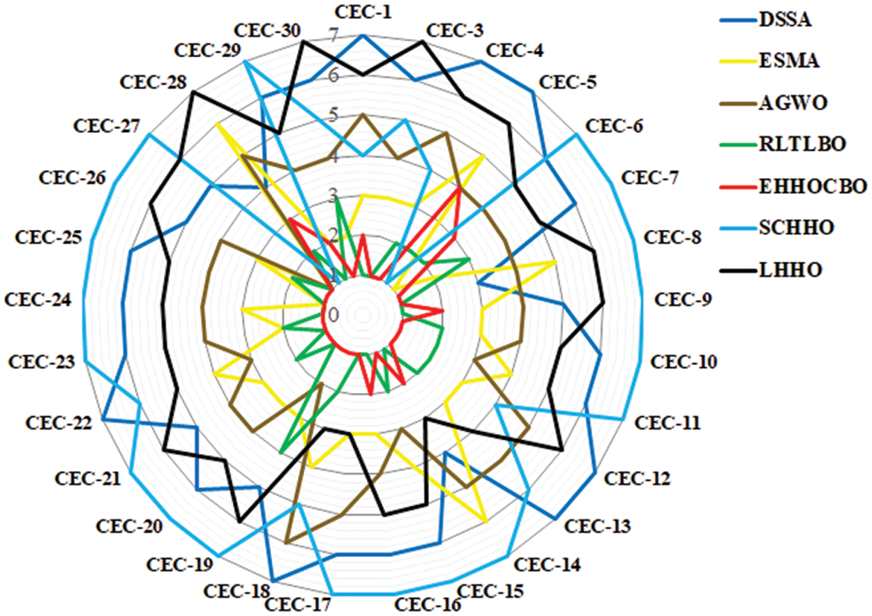
Figure 7: Ranking on IEEE CEC2017 test function
5 EHHOCBO for Addressing Engineering Problems
This section uses EHHOCBO to solve four common engineering problems in the structure field. Engineering problem testing validates the applicability and black-box nature of meta-heuristic algorithms in real-world constrained optimization. The four problems used are the cantilever beam design problem, speed reducer design problem, welded beam design problem, and rolling element bearing design problem. This paper introduces the death penalty function [60] to deal with those non-feasible candidate solutions under equality and inequality constraints. The maximum number of iterations and population size are still set to 500 and 30, respectively. In this experiment, each algorithm runs independently 30 times. The detailed experimental results and discussions are as follows.
5.1 Cantilever Beam Design Problem
The cantilever beam design problem is a structural engineering design problem that is related to the weight optimization of a cantilever beam with square cross-section. One end of the cantilever beam is rigidly supported, and the vertical force acts on the free node of the cantilever. The beam comprises five hollow blocks with constant thickness, and its height is a decision variable. The structure of the cantilever beam is shown in Fig. 8, and the mathematical formula of the problem is as follows:
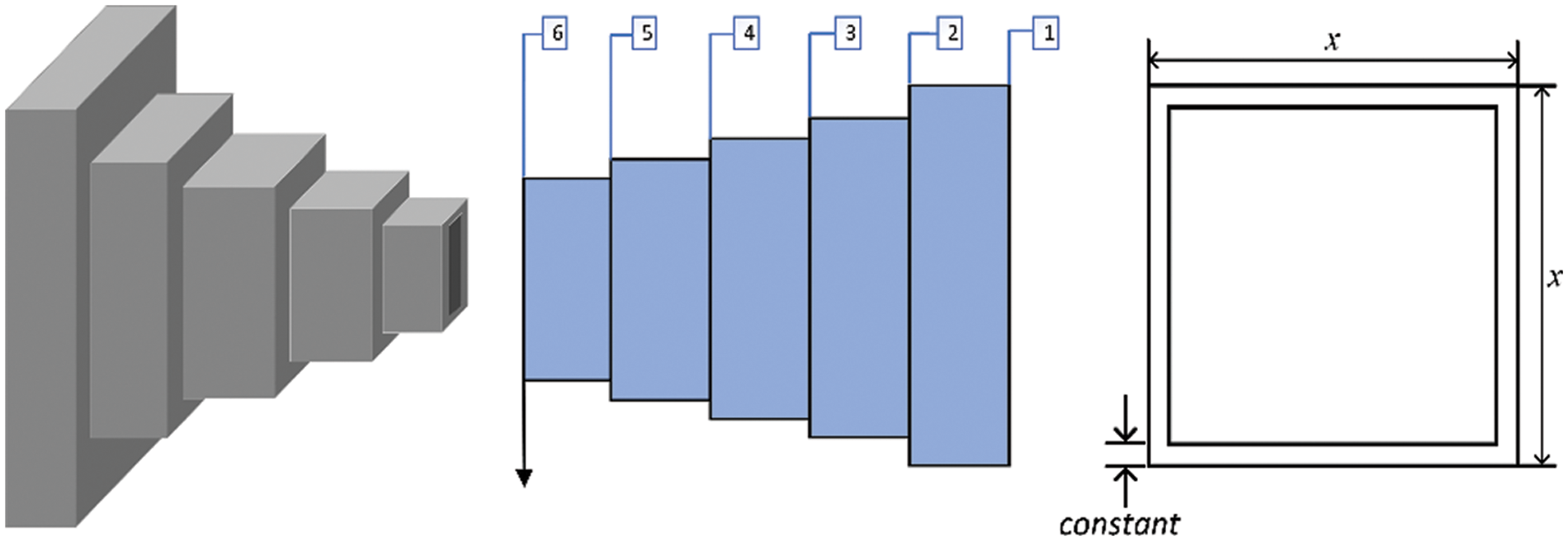
Figure 8: Schematic diagram of cantilever beam design problem
Consider:
Minimize:
Subject to:
Variable range:
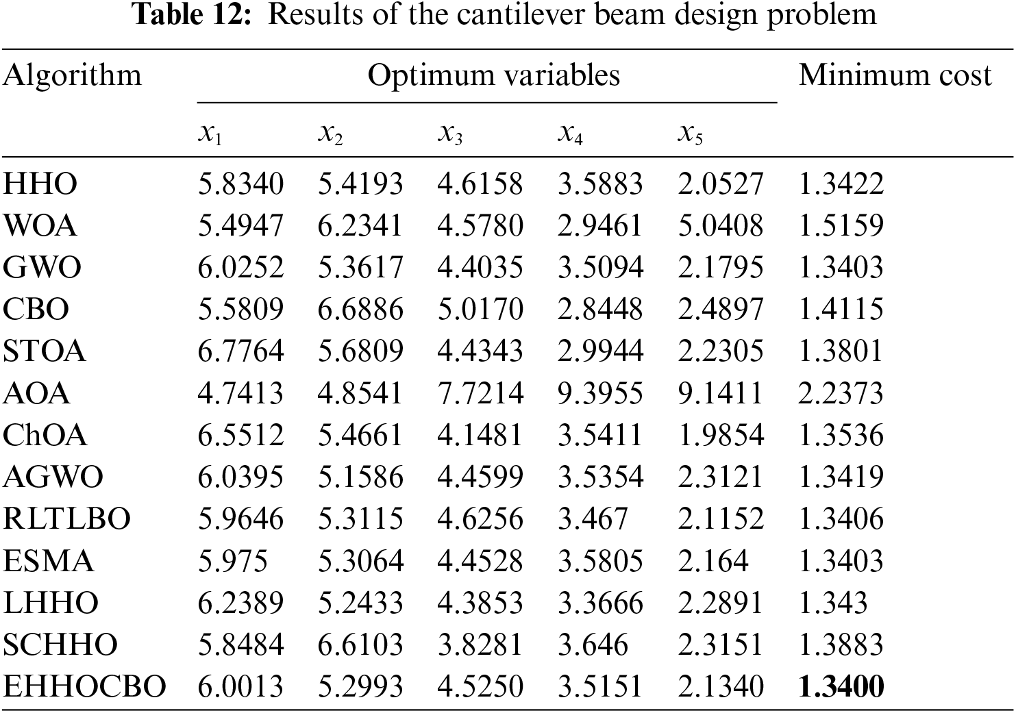
The optimization results of EHHOCBO and other algorithms for the cantilever beam design problem are presented in Table 12. The results show that EHHOCBO proposed in this paper achieves the best design. Its performance is significantly improved compared with the basic CBO and HHO algorithms. Therefore, we believe that the EHHOCBO algorithm has good potential for solving such problems.
5.2 Speed Reducer Design Problem
The objective of this optimization problem is to minimize the weight of the reduction gear subject to 11 constraints. The decision variables in this problem are the width of the tooth face
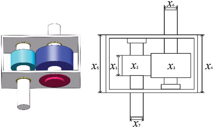
Figure 9: Schematic diagram of speed reducer design problem
Consider:
Minimize:
Subject to:
Variable range:
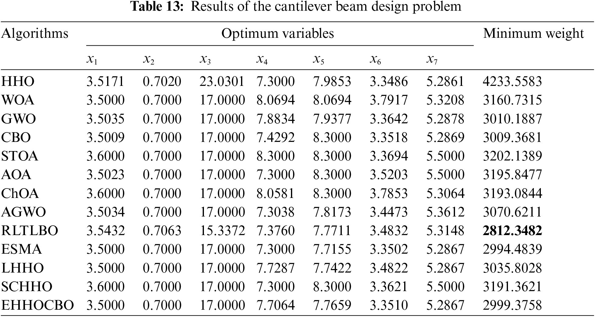
The results of this experiment are recorded in Table 13. The results show that the minimum weight of EHHOCBO is slightly worse than that of RLTLBO and ESMA algorithms. Although EHHOCBO could have better design results, it achieves relatively good performance. Therefore, it is reasonable to believe that the proposed hybrid technique is suitable for solving the speed reducer design problem.
5.3 Welded Beam Design Problem
The purpose of the design problem of the welded beam is to reduce the manufacturing cost of the design as much as possible under the constraint of meeting the beam’s shear stress, bending stress, bending load, end deviation, and boundary conditions. The problem can be described as an optimization design problem with four decision variables. The four decision variables are length
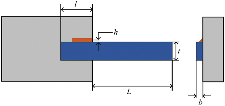
Figure 10: Schematic diagram of the welded beam design problem
Consider:
Minimize:
Subject to:
Variable range:
where
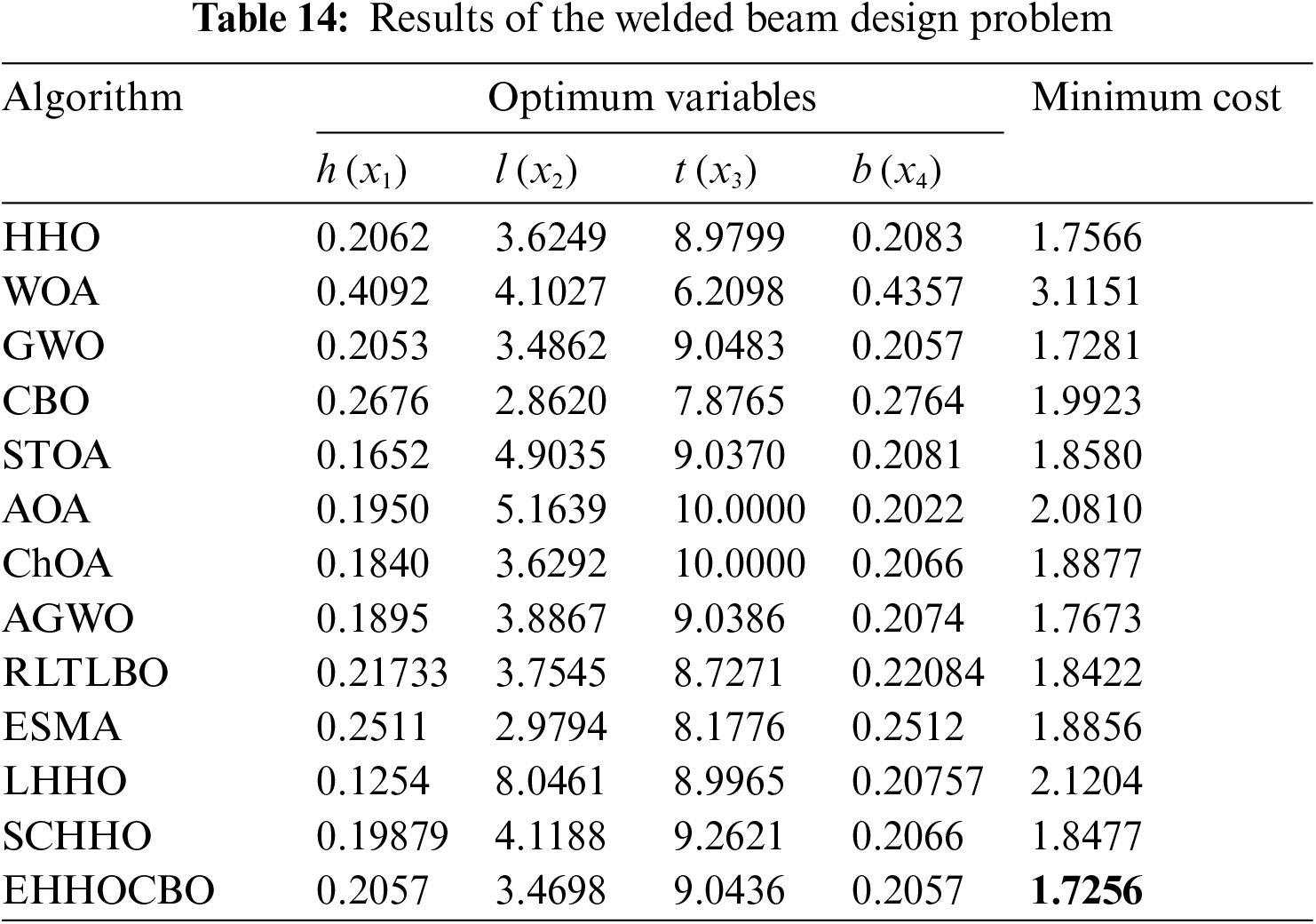
The results of the experiment are shown in Table 14. EHHOCBO obtaines the lowest manufacturing cost of 1.7256 under the corresponding parameters
5.4 Rolling Element Bearing Design Problem
The objective of the rolling element bearing design problem is to find the maximum dynamic load capacity of a bearing subject to more than ten decision parameters. The decision parameters are pitch diameter
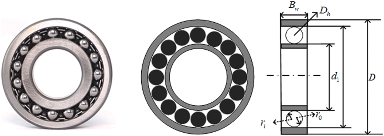
Figure 11: Schematic diagram of rolling element bearing design problem
Maximize:
Subject to:
where
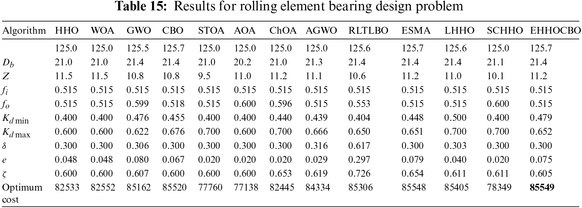
The results of this experiment are reported in Table 15. It can be seen from this table that compared with other classical algorithms, the proposed EHHOCBO provides the best fitness value of 85549.
The above experiments show that EHHOCBO has advantages in solving practical engineering problems. This is attributed to the combination of HHO and CBO, as well as the introduction of the ensemble mutation strategy and refracted opposition-based learning, which improves the proposed method’s searchability significantly.
6 Conclusion and Future Directions
Considering the respective characteristics of the HHO algorithm and CBO algorithm, a new improved hybrid algorithm named EHHOCBO is proposed in this paper. First, the leader mechanism of CBO is introduced in the initialization phase of HHO to provide a good basis for global search and enhance the exploration ability of the algorithm. Then, an ensemble mutation strategy is employed to increase the population diversity and further boost the exploration trend. Finally, refracted opposition-based learning is used to update the optimal solution to expand the search range and avoid the algorithm falling into the local optima. In order to fully evaluate the performance of the proposed algorithm, EHHOCBO was compared with the basic HHO, CBO algorithm, and other meta-heuristic algorithms based on classical benchmark functions and the IEEE CEC2017 test suite. Wilcoxon’s rank sum test verified the significance of the experimental results. Through a series of numerical statistics, it is verified that the EHHOCBO algorithm has significantly improved in terms of accuracy, convergence speed, stability, and avoidance of falling into local optimum solutions. In addition, four engineering problems were used to verify the applicability of the EHHOCBO algorithm. Experiments show that the algorithm can effectively provide competitive solutions for these real-life engineering problems.
Although the EHHOCBO algorithm proposed in this paper has been significantly improved over the basic HHO and CBO algorithms, there is still room for further improvement in its performance on IEEE CEC2017 test functions. The EHHOCBO algorithm still suffers from the major limitation of excessive computation time and needs to be improved. It is believed that this situation can be alleviated by introducing several parallel mechanisms, such as master-slave models, cellular models and coordination strategies. In future work, we aim to further improve the performance of the EHHOCBO algorithm by developing new improvement strategies and parallelism mechanisms while reducing the total time consumption. And we hope to make the parameter settings more reasonable by incorporating parameter adaptive control. In addition, we believe it would also be interesting to implement EHHOCBO to solve more practical optimization problems such as feature selection, path planning, predictive modeling, image segmentation, etc. [61]. We will enhance our work in this area.
Acknowledgement: The authors are grateful to the editor and reviewers for their constructive comments and suggestions, which have improved the presentation.
Funding Statement: This work is financially supported by the National Natural Science Foundation of China under Grant 52075090, Key Research and Development Program Projects of Heilongjiang Province under Grant GA21A403, the Fundamental Research Funds for the Central Universities under Grant 2572021BF01, and Natural Science Foundation of Heilongjiang Province under Grant YQ2021E002.
Conflicts of Interest: The authors declare that they have no conflicts of interest to report regarding the present study.
References
1. Xiao, Y., Sun, X., Guo, Y., Li, S., Zhang, Y. et al. (2022). An improved gorilla troops optimizer based on lens opposition-based learning and adaptive beta-Hill climbing for global optimization. Computer Modeling in Engineering & Sciences, 131(2), 815–850. https://doi.org/10.32604/cmes.2022.019198 [Google Scholar] [CrossRef]
2. Xiao, Y., Sun, X., Guo, Y., Cui, H., Wang, Y. et al. (2022). An enhanced honey badger algorithm based on Levy flight and refraction opposition-based learning for engineering design problems. Journal of Intelligent & Fuzzy Systems, 43(4), 4517–4540. https://doi.org/10.3233/JIFS-213206 [Google Scholar] [CrossRef]
3. Zhang, X. C., Zhao, K., Niu, Y. (2020). Improved Harris hawks optimization based on adaptive cooperative foraging and dispersed foraging strategies. IEEE Access, 8, 160297–160314. https://doi.org/10.1109/ACCESS.2020.3013332 [Google Scholar] [CrossRef]
4. Boussaid, I., Lepagnot, J., Siarry, P. (2013). A survey on optimization metaheuristics. Information Sciences, 237, 82–117. https://doi.org/10.1016/j.ins.2013.02.041 [Google Scholar] [CrossRef]
5. Jia, H. M., Li, Y., Sun, K. J., Cao, N., Zhou, H. M. (2021). Hybrid sooty tern optimization and differential evolution for feature selection. Computer Systems Science and Engineering, 39(3), 321–335. https://doi.org/10.32604/csse.2021.017536 [Google Scholar] [CrossRef]
6. Fan, Q. S., Huang, H. S., Yang, K., Zhang, S. S., Yao, L. G. et al. (2021). A modified equilibrium optimizer using opposition-based learning and novel update rules. Expert Systems with Applications, 170(9), 114575. https://doi.org/10.1016/j.eswa.2021.114575 [Google Scholar] [CrossRef]
7. Hussain, K., Mohd Salleh, M. N., Cheng, S., Shi, Y. (2019). Metaheuristic research: A comprehensive survey. Artificial Intelligence Review, 52(4), 2191–2233. https://doi.org/10.1007/s10462-017-9605-z [Google Scholar] [CrossRef]
8. Zheng, R., Jia, H. M., Wang, S., Liu, Q. X. (2022). Enhanced slime mould algorithm with multiple mutation strategy and restart mechanism for global optimization. Journal of Intelligent & Fuzzy Systems, 42(6), 5069–5083. https://doi.org/10.3233/JIFS-211408 [Google Scholar] [CrossRef]
9. Xiao, Y., Guo, Y., Cui, H., Wang, Y., Li, J. et al. (2022). IHAOAVOA: An improved hybrid aquila optimizer and African vultures optimization algorithm for global optimization problems. Mathematical Biosciences and Engineering, 19(11), 10963–11017. https://doi.org/10.3934/mbe.2022512 [Google Scholar] [PubMed] [CrossRef]
10. Zhong, K. Y., Zhou, G., Deng, W., Zhou, Y. Q., Luo, Q. F. (2021). MOMPA: Multi-objective marine predator algorithm. Computer Methods in Applied Mechanics and Engineering, 385(1), 114029. https://doi.org/10.1016/j.cma.2021.114029 [Google Scholar] [CrossRef]
11. Yu, G., Wang, H., Zhou, H. Z., Zhao, S. S., Wang, Y. (2021). An efficient firefly algorithm based on modified search strategy and neighborhood attraction. International Journal of Intelligent Systems, 36(8), 4346–4363. https://doi.org/10.1002/int.22462 [Google Scholar] [CrossRef]
12. Xiao, Y., Sun, X., Zhang, Y., Guo, Y., Wang, Y. et al. (2021). An improved slime mould algorithm based on tent chaotic mapping and nonlinear inertia weight. International Journal of Innovative Computing, Information and Control, 17(6), 2151–2176. https://doi.org/10.24507/ijicic.17.06.2151 [Google Scholar] [CrossRef]
13. Nguyen, T. T., Wang, H. J., Dao, T. K., Pan, J. S., Liu, J. H. et al. (2020). An improved slime mold algorithm and its application for optimal operation of cascade hydropower stations. IEEE Access, 8, 226754–226772. https://doi.org/10.1109/ACCESS.2020.3045975 [Google Scholar] [CrossRef]
14. Dehghani, M., Montazeri, Z., Givi, H., Guerrero, J., Dhiman, G. (2020). Darts game optimizer: A new optimization technique based on darts game. International Journal of Intelligent Engineering and Systems, 13(5), 286–294. https://doi.org/10.22266/ijies2020.1031.26 [Google Scholar] [CrossRef]
15. Hamed, A. Y., Alkinani, M. H., Hassan, M. R. (2020). A genetic algorithm optimization for multi-objective multicast routing. Intelligent Automation and Soft Computing, 26(6), 1201–1216. https://doi.org/10.32604/iasc.2020.012663 [Google Scholar] [CrossRef]
16. Storn., R., Price., K. (1997). Differential evolution–A simple and efficient heuristic for global optimization over continuous spaces. Journal of Global Optimization, 11(4), 341–359. https://doi.org/10.1023/A:1008202821328 [Google Scholar] [CrossRef]
17. Beyer, H. G., Schwefel, H. P. (2002). Evolution strategies. A comprehensive introduction. Natural Computing, 1(1), 3–52. https://doi.org/10.1023/A:1015059928466 [Google Scholar] [CrossRef]
18. Kirkpatrick, S., Gelatt, C. D., Vecchi, M. P. (1983). Optimization by simulated annealing. Science, 220(4598), 671–680. https://doi.org/10.1126/science.220.4598.671 [Google Scholar] [PubMed] [CrossRef]
19. Mirjalili, S., Mirjalili, S. M., Hatamlou, A. (2016). Multi-verse optimizer: A nature-inspired algorithm for global optimization. Neural Computing & Applications, 27(2), 495–513. https://doi.org/10.1007/s00521-015-1870-7 [Google Scholar] [CrossRef]
20. Zhao, W. G., Wang, L. Y., Zhang, Z. X. (2019). Atom search optimization and its application to solve a hydrogeologic parameter estimation problem. Knowledge-Based Systems, 163(4598), 283–304. https://doi.org/10.1016/j.knosys.2018.08.030 [Google Scholar] [CrossRef]
21. Abualigah, L., Diabat, A., Mirjalili, S., Abd Elaziz, M., Gandomi, A. H. (2021). The arithmetic optimization algorithm. Computer Methods in Applied Mechanics and Engineering, 376(2), 113609. https://doi.org/10.1016/j.cma.2020.113609 [Google Scholar] [CrossRef]
22. Kennedy, J., Eberhart, R. (1995). Particle swarm optimization. Proceedings of ICNN’95—International Conference on Neural Networks, pp. 1942–1948. Perth, WA, Australia. https://doi.org/10.1109/ICNN.1995.488968 [Google Scholar] [CrossRef]
23. Mirjalili, S. (2016). SCA: A sine cosine algorithm for solving optimization problems. Knowledge-Based Systems, 96(63), 120–133. https://doi.org/10.1016/j.knosys.2015.12.022 [Google Scholar] [CrossRef]
24. Dhiman, G., Kaur, A. (2019). STOA: A bio-inspired based optimization algorithm for industrial engineering problems. Engineering Applications of Artificial Intelligence, 82(2), 148–174. https://doi.org/10.1016/j.engappai.2019.03.021 [Google Scholar] [CrossRef]
25. Khishe, M., Mosavi, M. R. (2020). Chimp optimization algorithm. Expert Systems with Applications, 149(1), 113338. https://doi.org/10.1016/j.eswa.2020.113338 [Google Scholar] [CrossRef]
26. Abualigah, L., Yousri, D., Abd Elaziz, M., Ewees, A. A., Al-qaness, M. A. A. et al. (2021). Aquila optimizer: A novel meta-heuristic optimization algorithm. Computers & Industrial Engineering, 157(11), 107250. https://doi.org/10.1016/j.cie.2021.107250 [Google Scholar] [CrossRef]
27. Mirjalili, S. (2016). Dragonfly algorithm: A new meta-heuristic optimization technique for solving single-objective, discrete, and multi-objective problems. Neural Computing & Applications, 27(4), 1053–1073. https://doi.org/10.1007/s00521-015-1920-1 [Google Scholar] [CrossRef]
28. Arora, S., Singh, S. (2019). Butterfly optimization algorithm: A novel approach for global optimization. Soft Computing, 23(3), 715–734. https://doi.org/10.1007/s00500-018-3102-4 [Google Scholar] [CrossRef]
29. Li, S. M., Chen, H. L., Wang, M. J., Heidari, A. A., Mirjalili, S. (2020). Slime mould algorithm: A new method for stochastic optimization. Future Generation Computer Systems, 111(Supplement C), 300–323. https://doi.org/10.1016/j.future.2020.03.055 [Google Scholar] [CrossRef]
30. Mirjalili, S., Lewis, A. (2016). The whale optimization algorithm. Advances in Engineering Software, 95(12), 51–67. https://doi.org/10.1016/j.advengsoft.2016.01.008 [Google Scholar] [CrossRef]
31. Mirjalili, S., Mirjalili, S. M., Lewis, A. (2014). Grey wolf optimizer. Advances in Engineering Software, 69, 46–61. https://doi.org/10.1016/j.advengsoft.2013.12.007 [Google Scholar] [CrossRef]
32. Dhiman, G., Kumar, V. (2019). Seagull optimization algorithm: Theory and its applications for large-scale industrial engineering problems. Knowledge-Based Systems, 165(25), 169–196. https://doi.org/10.1016/j.knosys.2018.11.024 [Google Scholar] [CrossRef]
33. Abdollahzadeh, B., Gharehchopogh, F. S., Mirjalili, S. (2021). Artificial gorilla troops optimizer: A new nature-inspired metaheuristic algorithm for global optimization problems. International Journal of Intelligent Systems, 36(10), 5887–5958. https://doi.org/10.1002/int.22535 [Google Scholar] [CrossRef]
34. Goncalves, M. S., Lopez, R. H., Miguel, L. F. F. (2015). Search group algorithm: A new metaheuristic method for the optimization of truss structures. Computers & Structures, 153(12), 165–184. https://doi.org/10.1016/j.compstruc.2015.03.003 [Google Scholar] [CrossRef]
35. Wolpert, D. H., Macready, W. G. (1997). No free lunch theorems for optimization. IEEE Transactions on Evolutionary Computation, 1(1), 67–82. https://doi.org/10.1109/4235.585893 [Google Scholar] [CrossRef]
36. Jia, H. M., Sun, K. J., Zhang, W. Y., Leng, X. (2022). An enhanced chimp optimization algorithm for continuous optimization domains. Complex & Intelligent Systems, 8(1), 65–82. https://doi.org/10.1007/s40747-021-00346-5 [Google Scholar] [CrossRef]
37. Debnath, S., Baishya, S., Sen, D., Arif, W. (2021). A hybrid memory-based dragonfly algorithm with differential evolution for engineering application. Engineering with Computers, 37(4), 2775–2802. https://doi.org/10.1007/s00366-020-00958-4 [Google Scholar] [CrossRef]
38. Ziyu, T., Dingxue, Z. (2009). A modified particle swarm optimization with an adaptive acceleration coefficients. 2009 Asia-Pacific Conference on Information Processing, pp. 330–332. Shenzhen, China. https://doi.org/10.1109/APCIP.2009.217 [Google Scholar] [CrossRef]
39. Li, S. L., Li, X. B., Chen, H., Zhao, Y. X., Dong, J. W. (2021). A novel hybrid hunger games search algorithm with differential evolution for improving the behaviors of non-cooperative animals. IEEE Access, 9, 164188–164205. https://doi.org/10.1109/ACCESS.2021.3132617 [Google Scholar] [CrossRef]
40. Jia, H., Jiang, Z., Li, Y. (2022). Simultaneous feature selection optimization based on improved bald eagle search algorithm. Control and Decision, 37(2), 445–454. https://doi.org/10.13195/j.kzyjc.2020.1025 [Google Scholar] [CrossRef]
41. Heidari, A. A., Mirjalili, S., Faris, H., Aljarah, I., Mafarja, M. et al. (2019). Harris hawks optimization: Algorithm and applications. Future Generation Computer Systems, 97, 849–872. https://doi.org/10.1016/j.future.2019.02.028 [Google Scholar] [CrossRef]
42. Fan, Q., Chen, Z. J., Xia, Z. H. (2020). A novel quasi-reflected Harris hawks optimization algorithm for global optimization problems. Soft Computing, 24(19), 14825–14843. https://doi.org/10.1007/s00500-020-04834-7 [Google Scholar] [CrossRef]
43. Dokeroglu, T., Sevinc, E. (2022). An island parallel Harris hawks optimization algorithm. Neural Computing and Applications, 34(21), 18341–18368. https://doi.org/10.1007/s00521-022-07367-2 [Google Scholar] [CrossRef]
44. Wang, S. A., Jia, H. M., Abualigah, L., Liu, Q. X., Zheng, R. (2021). An improved hybrid aquila optimizer and Harris hawks algorithm for solving industrial engineering optimization problems. Processes, 9(9), 1551. https://doi.org/10.3390/pr9091551 [Google Scholar] [CrossRef]
45. Naruei, I., Keynia, F. (2021). A new optimization method based on COOT bird natural life model. Expert Systems with Applications, 183(2), 115352. https://doi.org/10.1016/j.eswa.2021.115352 [Google Scholar] [CrossRef]
46. Huang, Y. H., Zhang, J., Wei, W., Qin, T., Fan, Y. C. et al. (2022). Research on coverage optimization in a WSN based on an improved COOT bird algorithm. Sensors, 22(9), 3383. https://doi.org/10.3390/s22093383 [Google Scholar] [PubMed] [CrossRef]
47. Wang, Y., Cai, Z. X., Zhang, Q. F. (2011). Differential evolution with composite trial vector generation strategies and control parameters. IEEE Transactions on Evolutionary Computation, 15(1), 55–66. https://doi.org/10.1109/TEVC.2010.2087271 [Google Scholar] [CrossRef]
48. Long, W., Wu, T. B., Jiao, J. J., Tang, M. Z., Xu, M. (2020). Refraction-learning-based whale optimization algorithm for high-dimensional problems and parameter estimation of PV model. Engineering Applications of Artificial Intelligence, 89(1), 103457. https://doi.org/10.1016/j.engappai.2019.103457 [Google Scholar] [CrossRef]
49. Tizhoosh, H. R. (2005). Opposition-based learning: A new scheme for machine intelligence. International Conference on Computational Intelligence for Modelling, Control and Automation and International Conference on Intelligent Agents, Web Technologies and Internet Commerce, pp. 695–701. Vienna, Austria. https://doi.org/10.1109/CIMCA.2005.1631345 [Google Scholar] [CrossRef]
50. Sihwail, R., Omar, K., Ariffin, K. A. Z., Tubishat, M. (2020). Improved harris hawks optimization using elite opposition-based learning and novel search mechanism for feature selection. IEEE Access, 8, 121127–121145. https://doi.org/10.1109/ACCESS.2020.3006473 [Google Scholar] [CrossRef]
51. Digalakis, J. G., Margaritis, K. G. (2001). On benchmarking functions for genetic algorithms. International Journal of Computer Mathematics, 77(4), 481–506. https://doi.org/10.1080/00207160108805080 [Google Scholar] [CrossRef]
52. Cheng, R., Li, M., Tian, Y., Zhang, X., Jin, Y. et al. (2017). Benchmark functions for the CEC’2017 competition on evolutionary many-objective optimization. http://hdl.handle.net/2086/13857 [Google Scholar]
53. García, S., Fernández, A., Luengo, J., Herrera, F. (2010). Advanced nonparametric tests for multiple comparisons in the design of experiments in computational intelligence and data mining: Experimental analysis of power. Information Sciences, 180(10), 2044–2064. https://doi.org/10.1016/j.ins.2009.12.010 [Google Scholar] [CrossRef]
54. Jena, B., Naik, M. K., Wunnava, A., Panda, R. (2021). A differential squirrel search algorithm. In: Das, S., Mohanty, M. N. (Eds.Advances in intelligent computing and communication, pp. 143–152. Singapore: Springer. [Google Scholar]
55. Naik, M. K., Panda, R., Abraham, A. (2021). An entropy minimization based multilevel colour thresholding technique for analysis of breast thermograms using equilibrium slime mould algorithm. Applied Soft Computing, 113, 107955. https://doi.org/10.1016/j.asoc.2021.107955 [Google Scholar] [CrossRef]
56. Ma, C., Huang, H., Fan, Q., Wei, J., Du, Y. et al. (2022). Grey wolf optimizer based on aquila exploration method. Expert Systems with Applications, 205, 117629. https://doi.org/10.1016/j.eswa.2022.117629 [Google Scholar] [CrossRef]
57. Wu, D., Wang, S., Liu, Q., Abualigah, L., Jia, H. (2022). An improved teaching-learning-based optimization algorithm with reinforcement learning strategy for solving optimization problems. Computational Intelligence and Neuroscience, 2022, 1535957. https://doi.org/10.1155/2022/1535957 [Google Scholar] [PubMed] [CrossRef]
58. Naik, M. K., Panda, R., Wunnava, A., Jena, B., Abraham, A. (2021). A leader Harris hawks optimization for 2-D Masi entropy-based multilevel image thresholding. Multimedia Tools and Applications, 80(28), 35543–35583. https://doi.org/10.1007/s11042-020-10467-7 [Google Scholar] [CrossRef]
59. Hussain, K., Neggaz, N., Zhu, W., Houssein, E. H. (2021). An efficient hybrid sine-cosine Harris hawks optimization for low and high-dimensional feature selection. Expert Systems with Applications, 176, 114778. https://doi.org/10.1016/j.eswa.2021.114778 [Google Scholar] [CrossRef]
60. Coello Coello, C. A. (2002). Theoretical and numerical constraint-handling techniques used with evolutionary algorithms: A survey of the state of the art. Computer Methods in Applied Mechanics and Engineering, 191(11), 1245–1287. https://doi.org/10.1016/S0045-7825(01)00323-1 [Google Scholar] [CrossRef]
61. Shehab, M., Mashal, I., Momani, Z., Shambour, M. K. Y., Al-Badareen, A. et al. (2022). Harris hawks optimization algorithm: Variants and applications. Archives of Computational Methods in Engineering, 29(7), 5579–5603. https://doi.org/10.1007/s11831-022-09780-1 [Google Scholar] [CrossRef]
Cite This Article
 Copyright © 2023 The Author(s). Published by Tech Science Press.
This work is licensed under a Creative Commons Attribution 4.0 International License , which permits unrestricted use, distribution, and reproduction in any medium, provided the original work is properly cited.
 Downloads
 Citation Tools