Peridynamic Study on Fracture Mode and Crack Propagation Path of a Plate with Multiple Cracks Subjected to Uniaxial Tension

1  Introduction

Peridynamics (PD) is a reformulation of the classical continuum mechanics [1–7]. Based on the relaxation for the continuity of the displacement field, PD allows for discontinuities in the solution of the motion equation [1,2]. Therefore, PD can be utilized to conveniently simulate the crack initiation, branch, and propagation through terminating bond interactions without initially specifying the factitious crack and crack path [8,9].

The interest in PD has been growing due to its unparalleled ability to analyze various complex crack problems [10]. Adopting PD, Silling et al. simulated the stretching and dynamic tearing of membranes [11]. Bobaru et al. [12,13] and Ha et al. [14,15] used PD modeling to investigate the dynamic fracture of materials, and analyzed the crack propagation speed, crack path, and crack branching [14,15]. Dipasquale et al. studied the crack-path dependence on the grid orientation and proposed adaptive refinement techniques applied only where crack propagation is taking place [16,17]. Madenci et al. predicted the pre-existing crack propagation paths in a four-point shear specimen and a compact tension test specimen with a sink and a missing hole under complex loading conditions [18]. Wang et al. simulated the initiation, propagation, and coalescence of the pre-existing flaws in rocks subjected to compressive loads [19]. Gu et al. used voronoi-based peridynamics to analyze the crack path and propagation speed [20]. Lee et al. systematically investigated the initiation and propagation of basic crack types between two flaws, as well as the coalescence and interaction mechanisms of newly growing cracks in rock-like material under uniaxial compression [21]. Wang et al. put forward the novel conjugated bond-based peridynamics to investigate the initiation, propagation and coalescence behaviors of cracks in brittle solids [22,23]. Rabczuk et al. found a new penalty method to analyze the contact problems of compressive fractures in the four-point shear test and the indirect tensile (Brazilian) test of rock disks with one or multiple initial cracks [24]. Zhang et al. adopted a modified axisymmetric ordinary state-based peridynamic model introducing the shear effects to simulate the initiation and propagation of cracks under the axisymmetrical conditions [25]. Using a coupled FEM–PD approach, Ni et al. simulated the crack propagation through typical numerical examples [26]. Shojaei et al. put forward a radically new strategy to couple grids with different spacing to investigate the crack propagation in brittle materials [27].

Shou et al. proposed an extended non-ordinary state-based peridynamics to investigate the initiation, propagation and coalescence of 3D pre-existing flaws in PMMA specimens subjected to uniaxial compressive loads [28]. Zhou et al. [29] introduced tangent bonds into the bond-based peridynamic formulation to solve the limitation of fixed Poisson’s ratio and verified its accuracy by simulating the initiation, propagation, and coalescence of cracks in brittle rock materials subjected to compressive loads. Huang et al. completed the analysis to an improved bond-based material model for the elastic deformation and quasi-static fracture analysis within the framework of PD, in which local damping is implemented into the peridynamic motion equation [30]. Gu et al. simulated the fracture process of a uniaxial tensile plate with a circle hole and the propagation and coalescence of cracks in a rock subjected to biaxial tension [31]. Ni et al. investigated crack propagation in a pre-cracked square plate with a centrally circular hole and an off-central circular hole under tension [32]. Huang et al. proposed the extended step-by-step loading bond-based peridynamic approach to calculate the quasi-static crack propagation in mode I and mode II of fracture [33]. Jo et al. introduced two-grid based sequential analysis algorithm for implicit peridynamics to find the quasi-static solutions of crack propagation problems [34]. Lai et al. developed a non-ordinary state-based peridynamic model to capture the damage propagation and other features of brittle fracture in ceramics or fracture in quasi-brittle materials in general [35].

Peridynamics has been used to simulate the failure of concrete structures. Zhang et al. proposed a novel coupled axial-shear interaction bond-slip model to simulate the damage behavior of reinforced concrete structures [36]. Song et al. developed a hybrid peridynamic and classical continuum mechanical model for the high-temperature damage and fracture analysis of concrete structures [37].

In present PD simulations, the external loads leading to crack initiation and growth are given by velocities or displacements of particles, rather than traction. This is due to the fact that it is very difficult to directly handle the traction and constraint imposed on the boundary surface of a body in peridynamics [38,39]. To prescribe the boundary traction, one has to set a fictitious boundary layer with thickness δ in which the displacement constraints and boundary traction are specified [3,40–42], and the “fictitious layer” is commonly placed outside the natural boundary surface [1,43].

Although such treatment can obtain good results, some unphysical artifacts often appear in computation owing to the approximate feature of the fictitious boundary layer [43]. Liu et al. found that the boundary effect becomes more conspicuous as the horizon increases, and the errors in calculating the equivalent Young’s modulus of the boundary layer also increase [44].

Parks et al. [45] introduced “ghost” particles to calculate pairwise forces through the boundaries of subdomains. Kilic et al. [46] pointed out that the traction or concentration forces cannot be directly applied on the boundary surface since their volume integrations are zero. They needed to be converted into equivalent body forces in the fictitious boundary layer. Oterkus et al. [47] proposed that boundary conditions can be easily enforced via a finite element model (FEM) of the subdomain containing boundaries through the merger of FEM and peridynamic theory. Wu et al. [48] and Wu et al. [49] put forward an approach based on the localized convex kernel approximation constructed by the mesh-free methods to impose boundary conditions in the state-based peridynamic method. Prudhomme et al. presented the so-called extended domain method and variable horizon method to enforce boundary conditions within the non-local bond-based peridynamic model [50]. Scabbia et al. introduced a layer of fictitious nodes around the body, the displacements of which are determined by multiple Taylor series expansions based on the nearest-node strategy to mitigate the surface effect and impose Dirichlet and Neumann boundary conditions in a peridynamic way [51]. Liu et al. proposed an extended fictitious node method to deal with cases with mixed boundary conditions of stress and displacement [52]. To handle nonhomogeneous traction loadings on complex boundaries, Yu et al. developed an asymptotically compatible meshfree discretization method by using local optimization problems to seek quadrature weights associated with a local neighborhood of particles [53].

Recently, Huang [38], Zhou et al. [54] and Yu et al. [55] proposed a new peridynamic motion equation in which the surface traction and displacement constraint are directly prescribed on the boundary surface. In theory, it is more natural and easier to deal with boundary conditions with the PD motion equation proposed by Huang. Following the new peridynamic motion equation, we will study the pre-existing crack initiation, propagation and failure in a square plate under tension loading.

The outline of the paper is as follows. In Section 2, we review the peridynamic motion equation with boundary conditions (PDB) and simplify the transfer functions of the boundary traction and of the boundary displacement constraint. In Section 3, the PD constitutive model and the damage-fracture model are discussed. The expressions of transfer functions of boundary constraints are determined. The numerical algorithm is given in Section 4 and the convergence of the numerical algorithm is verified in Section 5. In Section 6, we simulate single crack and multiple crack propagation in an elastic–brittle square plate subjected to uniaxial tension, respectively. The process of the crack propagation is investigated in detail. Finally, we close this paper with a summary.

2  Peridynamic Motion Equation with Traction Boundary Conditions

The peridynamic motion equation advanced by Silling [2] is inconsistent with the traction boundary condition. In order to offset this deficiency, a new peridynamic motion equation is proposed, which reads

∫∂Ωp[ L(x,x′)p(x′,t)+D(x,x′)y(x′,t) ]da(x′)+∫HxF(x,x′,t)dv(x′)+f(x,t)=ρ(x)v.(x,t)(1)

where ξ=x′−x and p(x′,t) is the traction prescribed on the boundary surface ∂Ωp and y(x′,t) is the displacement boundary condition, while L(x,x′) and D(x,x′) are the transfer functions of the boundary traction and of the boundary displacement constraint, respectively. They transfer the effects of the traction and the displacement constraint into every particle within material. Huang [38] has proved that Eq. (1) is compatible with the conservation law of momentum, when

∫ΩL(x,x′)dv(x)=1(2)

∫ΩD(x,x′)dv(x)=0(3)

and Eq. (1) is form-invariant under the Galileo transformation, if

∫∂ΩPD(x,x′)da(x′)=0(4)

Meanwhile, it has been certified that the traction p(x′,t), the displacement vector y(x′,t) and y(x,t) must satisfy the constraints below:

K(x,x′)[ y(x′,t)−y(x,t) ]=L(x,x′)p(x′,t)+D(x,x′)y(x′,t)(5)

so as to make Eq. (1) compatible with the conservation law of angular momentum. In fact, Eq. (5) can be regarded as a constitutive equation with relevance to the traction and displacement constraints on the boundary surface. So K(x,x′) is a stiffness coefficient.

When the displacement boundary condition y(x′,t)=y¯(x′,t)=x′+u¯(x′,t) is given on ∂Ω, ∂Ωp = 0. Here, y¯(x′,t) and u¯(x′,t) is the current position and displacement of material particles on ∂Ω. Eq. (1) returns to the original form of the peridynamic motion equation advanced by Silling [2], i.e.,

∫HxF(x,x′,t)dv(x′)+f(x,t)=ρ(x)v.(x,t)(6)

which can be also regarded as the peridynamic motion equation with the displacement boundary condition.

If the traction boundary condition p(x′,t)=p¯(x′,t) is given on ∂Ω, then we can solve Eq. (5) to acquire y(x′,t), that is

y(x′,t)=L(x,x′)K(x,x′)−D(x,x′)p¯(x′,t)+K(x,x′)K(x,x′)−D(x,x′)y(x,t).(7)

Different from the existing models, here p¯(x′,t) is the traction directly prescribed on ∂Ωp. Through the transfer functions, the effects of p¯(x′,t) are transmitted to every particle within peridynamic medium.

By inserting Eq. (7) in Eq. (1), the peridynamic motion equation with the traction boundary condition is given as follows:

∫∂Ωp[ α  (x,x′)p¯ (x′,t)+β (x,x′)y(x,t) ] da(x′)+∫HxF(x,x′,t) dv(x′)+f(x,t)=ρ (x)v.(x,t),(8)

where

α(x,x′)=K(x,x′)L(x,x′)K(x,x′)−D(x,x′),  β(x,x′)=K(x,x′)D(x,x′)K(x,x′)−D(x,x′)(9)

which is the peridynamic motion equation with the traction boundary condition.

Let ∂Ω=∂Ωu∪∂Ωp and ∂Ωu∩∂Ωp=∅, where ∂Ωu denotes the boundary surface subjected to the displacement constraint, while ∂Ωp is the boundary surface prescribed by traction.

Combining Eq. (6) with Eq. (8), we have

∫∂Ωp[ α(x,x′)p¯(x′,t)+β(x,x′)y(x,t) ] da(x′)+∫HxF(x,x′,t)dv(x′)+f(x,t)=ρ(x)v.(x,t)(10)

As a result, we acquire the peridynamic motion equation with the mixed boundary condition. For simplicity, we further assume that

K(x,x′)K(x,x′)−D(x,x′)=χ⇔K(x,x′)=χχ−1D(x,x′)(11)

where χ = (V − VB)/V, in which VB and V are the volume of boundary layer and the volume of the body, respectively. As a result, Eq. (10) leads to

χ∫∂Ωp[ L(x,x′)p¯(x′,t) ] da(x′)+∫HxF(x,x′,t)dv(x′)+f(x,t)=ρ(x)v.(x,t).(12)

When ∂Ωp = ∂Ω, Eq. (12) transforms from the peridynamic motion equation with the mixed boundary condition into the peridynamic motion equation with the traction boundary condition.

3  Peridynamic Constitutive Model

3.1 Bond-Based Constitutive Equation

The bond-based constitutive models have been established by Silling (BPD) [56]. Among them, prototype microelastic model constitutive equations for elastic deformation of isotropic materials are written as [43]

F(x,x′,t)={ C(| ξ |)eM, | ξ |≤δ0,    otherwise(13)

where

M=y(x′,t)−y(x,t)| y(x′,t)−y(x,t) |,  e=| y(x′,t)−y(x,t) |−| ξ |(14)

Here, C is the so-called micromodulus, and δ is the radius of Hx. According to the dimension of spatial configuration of body, C takes different value. The 2-dimensional prototype microelastic model reads

C(|ξ|)={9E/πhδ3|ξ|,planestress48E/5πhδ3|ξ|,plane strain(15)

In Eq. (15), E is the Young’s modulus, h is the thickness of plate.

3.2 Transfer Functions of Boundary Constraints

The transfer functions of boundary constraints contain the transfer function of the boundary displacement constraint D(x,x′) and the transfer function of the boundary traction L(x,x′) [38]. They can be constructed through many ways. For example, we can choose an integrable function q(| x−x′ |) to form L(x,x′)as follows:

L(x,x′)=q(| x−x′ |)∫Ωq(| x−x′ |)dv(x)(16)

In order to introduce as few undetermined functions as possible to represent L(x,x′), for a rectangular plate, we set

q(| x−x′ |)={ (1−(| x−x′ |)kδ),if(| x−x′ |≤δ), k=[ 18LWSδ ]0, otherwise(17)

where L and W are the length and width of the plate, respectively. S is the total length of the boundary prescribed by non-zone traction, δ is the horizon for the material. The sign [•] represents the integer function, so k is a positive integer. Physically, the effects caused by the prescribed displacement or traction at x′ on the boundary surface can be always transmitted to a point x in the interior of body through a path, even though there is a crack or void between the link between x′ and x. For simplicity, we assume that the intensity transmitted from x′ to x depends only on the distance between x′ and x, and attenuates with the increase of the distance.

3.3 Peridynamic Damage-Fracture Model

Peridynamics describes the deformation and motion due to the interaction between material points. Material points are connected to each other by bonds. The bond failure between material points is described by the bond stretch s, which is defined by [1–3,5]

s=| y′−y |−| x′−x || x′−x |=e| ξ |.(18)

When the deformation stretch exceeds the critical bond stretch s0, the bond between the two material points breaks irreversibly and permanently [1–3,5].

According to the peridynamic theory, the critical bond stretch s0 is related to the critical energy release rate G0 of materials [3,15,57]. For the 2D cases, the relation between s0 and G0 is represented as

s0={4πG09Eδ,plane stress5πG012Eδ,plane strain.(19)

As thus, the damage of the bond can be characterized by the scalar-valued function μ below [1–3,5]:

μ(t,ξ)={1,if s (t,ξ)<s00,otherwise.(20)

By (20), Eq. (13) is rewritten as

F(x,x′,t)={ μ(t,ξ)C(| ξ |)eM, | ξ |≤δ0,       otherwise(21)

Consequently, local damage φ at a material point is defined as [1,3,42]

φ(x,t)=1−∫Hxμ(x,t,ξ)dVξ∫HxdVξ.(22)

Note that the local damage ranges from 0 to 1. When φ=1, all the interactions initially associated with the point have been eliminated, while φ=0 means that all interactions are intact. The value of local damage represents the possibility of internal crack formation within a body [1,3,42].

4  Numerical Solution Method

The peridynamic motion equation is an integral equation, to find the analytical solution of which is very difficult [58]. Consequently, the numerical techniques are usually used to solve the peridynamic motion equation [43]. Firstly, a body is uniformly discretized into nodes with a certain volume in a reference configuration [3]. Unlike the finite element, all nodes form a freely deformable mesh. After discretion, the peridynamic motion equation (Eq. (12)) with the traction boundary condition can be approximately represented as

χ∑m=1Nbq(|xm−xi|)∑i=1Nq(|xm−xi|)Vip¯mAm+∑j,NC|xj+uj−xi−ui|−|xj−xi||xj−xi|⋅xj+uj−xi−ui|xj+uj−xi−ui|Vj+f(xi,t)=0i(23)

where m is the number of the one boundary node prescribed by non-zone traction, the subscripts denote the node numbers, Vj is the volume of the node j. If the boundary condition contains the displacement constraint, it is handled in the same way as the methods proposed by Silling [2,56,59].

The adaptive dynamic relaxation method [1,46] is adopted to solve Eq. (23). In this method, the velocity and displacement at the next time step can be obtained by employing explicit forward and backward difference techniques. The iterative scheme is expressed as follows:

u˙in+1=u¨inΔt+u˙in, u˙in+1=u¨inΔt+u˙in(24)

where n is the time step number.

In the explicit central difference form, the acceleration u¨in in Eq. (24) can be expressed as

u¨in=uin+1−2uin+uin−1Δt2(25)

where Δt is a constant time step.

5  Elastic Deformation Analysis and Convergence of a Square Plate under Uniaxial Tension

Take a square plate with the side length of 50 mm, as show in Fig. 1. The mass density of material is 8000 kg/m3, Poisson’s ratio v = 1/3 and Young’s modulus E = 192 GPa. In vertical direction, the plate is subjected to symmetrical loads of 200 MPa at the two ends. The constitutive equation is given by the prototype microelastic material model.

Figure 1: Schematics of square plate under uniaxial tension and its discretization

The square plate is discreated into a set of particles equally spaced from each other. In order to investigate the character of δ-convergence [1,12,15] of the improved peridynamics, four numerical examples with particle spacings Δx = 1, 0.5, 0.25 and 0.125 mm are used to demonstrate the δ-convergence when the ratio m = δ/Δx = 3.015 is fixed. The numerical results of the displacement at (0.1225, −0.1225) increasing with time steps are shown in Fig. 2. It is accessible to see that the computational results of four meshes tend to converge as the time steps reach 3000. Therefore, the time steps of 4000 will be adopted in the following calculation.

Figure 2: δ-convergence of calculated results with the change of meshes and time steps

In the elasticity, the displacements of the plate in Fig. 2 are analytically represented as

ux∗=−υpEx, uy∗=pEy(26)

where u*x and u*y are two displacement components. We compare the displacements given by Eq. (23) with the results calculated by Eq. (26). Fig. 3 shows the change of displacements at (−0.01225, −0.01225) with loading. From it, we see that the results calculated by Eqs. (23) and (26) are very close to each other.

Figure 3: Displacement components ux and uy at the collocation point (−0.01225, −0.01225) increasing with loading

The fracture of a square plate with small circular hole are also used to demonstrate the convergence [1,12,15] of the improved peridynamics. As shown in Fig. 4, the side length of the square plate is50 mm. The circular hole with the radius of r = 5 mm is located at the center of the square plate. The prototype microelastic brittle model is still utilized. The critical stretch s0 of bond failure is taken as 0.003.

Figure 4: Schematics of square plate under uniaxial tension

The square plate is discretized into 40000 (200 × 200) collocation points with the fixed grid spacing size Δx = 0.25 mm. The time step is set to Δt = 1 s.

As shown in Fig. 5, when the value of m is taken as 3.015, 4.015, 5.015 and 6.015 in turn, the numerical solutions of the square plate with small circular hole are closed to each other. The crack paths agree with the prediction of fracture mechanics and the size of cracking zones depends on the value of the horizon δ. The results demonstrate that the numerical algorithm is of convergence.

Figure 5: Convergence of calculated results with the change of horizon

6  Fracture of a Square Plate with Pre-Existing Cracks under Uniaxial Tension

Take a square plate with the side length of 50 mm. Let the Young’s modulus of the plate E = 30 GPa, the mass density ρ = 2460 kg/m3, the Possion’s ratio v = 1/3 and the critical energy release rate G0 = 110 J/m2 [35,60]. The constitutive behavior of the plate is characterized by the PMB model. In terms of Eq. (19), the critical bond stretch s0 corresponding to G0 = 110 J/m2 is 0.0026.

During the simulation, the square plate is discretized into 40000 (200 × 200) collocation points with the spacing of Δx = 0.25 mm. The horizontal size is specified as δ = 3.015Δx. The time step is set to Δt = 1 s. It should be emphasized that the surface correction and artificial boundary layer in the numerical algorithm are no longer needed due to the introduction of the transfer functions of boundary constraints. Next, we will calculate the fracture of the plate when different cracks are preset in the plate.

6.1 Single Crack

As illustrated in Fig. 6, a horizontal crack with the length of 10 mm is preset in the center of the square plate. The load is applied vertically to the upper and lower sides of the plate. The crack initiation and propagation are plotted in Fig. 7. We see that when the load reaches 14.6 MPa, the crack starts to propagate from both crack tips simultaneously until it penetrates the whole square plate. As expected, the crack propagation path is colinear with the initial crack.

Figure 6: Geometry and discretization of square plate with a central horizontal crack under tension

Figure 7: Damage diagram of the plate with a central horizontal crack: (a) initiation, (b) propagation, and (c) failure

Fig. 8 shows the plate with an inclined crack at the center. The initial length and orientation angle of the crack are 10 mm and 45°, respectively. When tension applied on the upper and lower sides of the plate reaches 15.9 MPa, the crack begins to deflect at the crack tips and then propagates in the in-plane opening mode until the plate breaks. Fig. 9 displays the crack propagation process described by the numerical solution of the peridynamic equation under the traction boundary conditions. At the crack tips, the fracture angle is 56°, which is consistent with the calculated result of fracture mechanics.

Figure 8: Geometry and discretization of square plate with an inclined central crack under tension

Figure 9: Damage diagram of the plate with an inclined central crack: (a) initiation, (b) propagation, and (c) failure

The plate preset an edge crack is shown in Fig. 10. Under the tension of 8.5 MPa, the crack propagates in a straight line and quickly penetrates the whole plate. Fig. 11 shows the propagation process of the edge crack.

Figure 10: Geometry of square plate with edge crack under tension

Figure 11: Damage diagram of the plate with an edge crack: (a) initiation, (b) propagation, and (c) failure

6.2 Double Crack

As illustrated in Fig. 12, two parallel cracks with the length of 10 mm are preset symmetrically in the square plate with the same size and model parameters as the plate in Fig. 6. The spacing between the two cracks is 25 mm. When the upper and lower sides of the plate are subjected to the uniaxial tension of 13.7 MPa, both cracks simultaneously start to propagate from their tips until the plate breaks into three pieces, as shown in Fig. 13. Interestingly, the propagation paths of the two cracks are not parallel straight lines, but curved lines that deviate from each other. They are closest in the middle and far away on the sides.

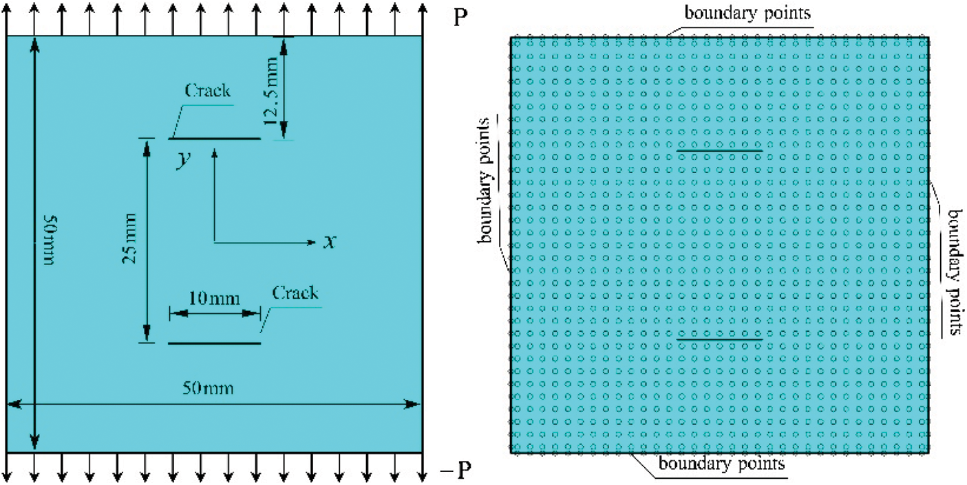
Figure 12: Geometry and discretization of square plate with two parallel cracks under tension

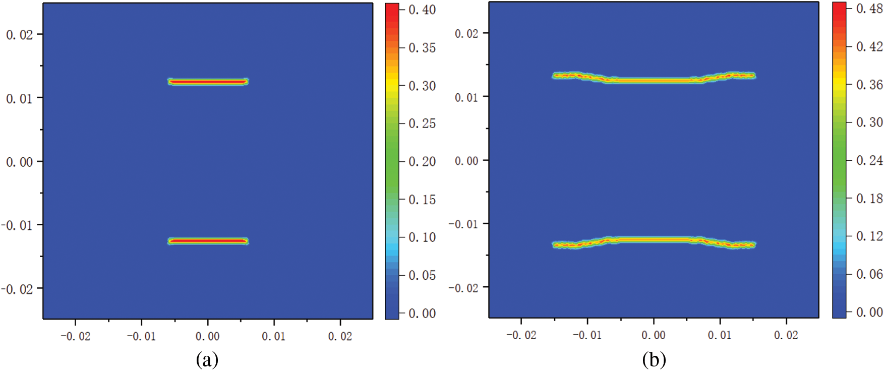
Figure 13: Damage diagram of the plate with two parallel cracks: (a) initiation, (b) propagation, and (c) failure

As illustrated in Fig. 14, two colinear edge cracks with the length of 5 mm are preset in the middle of the left and right sides of the square plate. The fracture process of the plate is shown in Fig. 15. We see that under the uniaxial tension of 8.5 MPa, the two edge cracks simultaneously propagate from the crack tip to the center of the plate. When the two cracks coalesce in the center of the plate, the plate breaks.

Figure 14: Geometry and discretization of square plate with two colinear edge cracks under tension

Figure 15: Damage diagram of the plate with two colinear edge cracks: (a) initiation, (b) propagation, and (c) failure

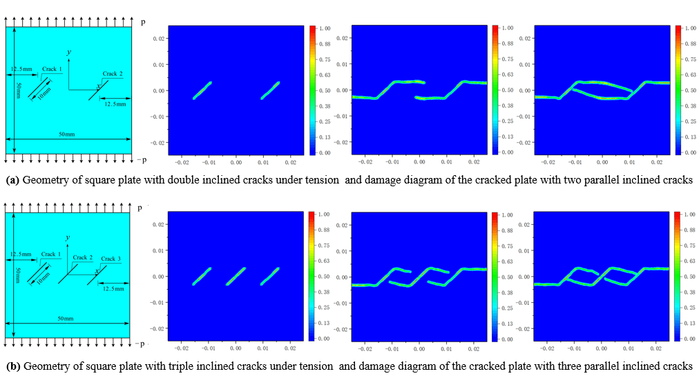
Two cracks are preset in the plate in two different configurations. One configuration is that two equal length parallel cracks are arranged in the plate at an angle of 45°, as shown in Fig. 16a. The other is a mirror symmetric configuration, as shown in Fig. 16b, in which two equal length cracks are inclined towards each other such that each crack forms an angle of 45° with the line joining their center. In the first configuration, the propagation process of crack 1 and crack 2 is illustrated in Fig. 17. We see that when p = 16.3 MPa, two cracks start to extend from their tips with the crack angle of about 56°. With the propagation of the cracks, the left tip of crack 1 and the right tip of crack 2 reach the left and right sides of the plate at the same time, but the plate is still not broken (seeing Fig. 17b). The right tip of crack 1 and the left tip of crack 2 continue to expand until they touch crack 2 and crack 1, respectively. At this moment, the plate is broken into three pieces, as shown in Fig. 17c.

Figure 16: Geometry of square plate with two inclined cracks under tension

Figure 17: Damage diagram of the plate with two parallel inclined cracks: (a) initiation, (b) propagation, and (c) failure

The crack propagation of the second configuration is shown in Fig. 18. With the uniaxial tension of the upper and lower sides reaching 16.9 MPa, two cracks simultaneously start to propagate rapidly from their tips with the crack angle of about 56°. While crack 1 and crack 2 coalesce into one crack in the middle of the plate, these two cracks also extend respectively from their other ends to the two edges of the plate, and thus the plate is split into two parts.

Figure 18: Damage diagram of the plate with two mirror symmetric cracks: (a) initiation, (b) propagation, and (c) failure

6.3 Triple Crack

Two configurations of three cracks in the plate are illustrated in Figs. 19a and 19b. In the first configuration, three equal length parallel cracks are placed horizontally and symmetrically in the plate, while in the second configuration, the upper and lower cracks are parallel to each other but the third crack is put in the middle between them at an angle of 45°.

Figure 19: Square plate with three cracks under uniaxial tension

The propagation process of cracks in the first configuration is shown in Fig. 20. Under the uniaxial tension of 14.7 MPa, we see that the upper and lower cracks propagate simultaneously to the left and right sides of the plate until they penetrate the whole plate. Meanwhile, the crack in the middle remains unchanged. These results are consistent with the prediction given by fracture mechanics. According to the fracture mechanics, in the Fig. 19a the stress intensity factors at the tips of the upper and lower cracks are equal, and they are greater than the stress intensity factors at the tips of the crack in the middle [61]. With the stress intensity factors reaching or exceeding the toughness of material, the upper and lower cracks will extend to the left and right sides of the plate in a path similar to that in Fig. 16c. With the propagation of the upper and lower crack, the strain energy is released in the plate. Therefore, the crack in the middle is no longer extended.

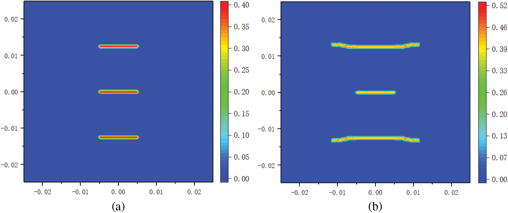
Figure 20: Damage diagram of the cracked plate as shown in Fig. 19a: (a) initiation, (b) propagation, and (c) failure

As shown in Fig. 21, the propagation of the cracks in the second configuration is similar to that in the first configuration. Under the uniaxial tension of 14.1 MPa, the upper and lower cracks extend to the left and right sides of the plate while the inclined crack in the middle remains unchanged. Different from the first configuration, in the second configuration, the propagation speed at both ends of the upper and lower cracks is different. The right end of the upper crack propagates slightly faster than the left end, while the propagation of the lower crack is just the opposite. As a result, Fig. 21b displays that the right end of the upper crack extends to the edge of the plate a little earlier than the left end, but the lower crack extends in the opposite way. From the point of view of fracture mechanics, this is because the inclination of the middle crack makes the stress intensity factor at the right tip of the upper crack larger than that at the left, while the stress intensity factor at the right tip of the lower crack is smaller than that at the left.

Figure 21: Damage diagram of the cracked plate as shown in Fig. 19b: (a) initiation, (b) propagation, and (c) failure

Fig. 22a illustrates the configuration of the plate in which three parallel cracks are preset at an angle of 45°. When the crack in the middle is changed to be placed horizontally, the configuration of the plate is shown in Fig. 22b. In the calculation, the plate is discretized into the same collocation point set as shown in Fig. 1.

Figure 22: Geometry of square plate with inclined cracks under tension

Under the tension of 16.2 MPa, the propagation of the cracks in Fig. 22a is exhibited in Fig. 23. At the beginning, three cracks extend form their tips at different fracture angles. From Figs. 23b and 23c, it is easy to see that the fracture angles at the left tip of crack 1 and the right tip of crack 3 are smaller than those at other tips. The left tip of crack 1 and the right tip of crack 3 firstly extend to two vertical sides of the plate. Subsequently, crack 2 and the other two ends of crack 1 and crack 3 continue to expand until the three cracks are fully connected. Finally, the plate is split into four pieces, two of which are much smaller than the other two.

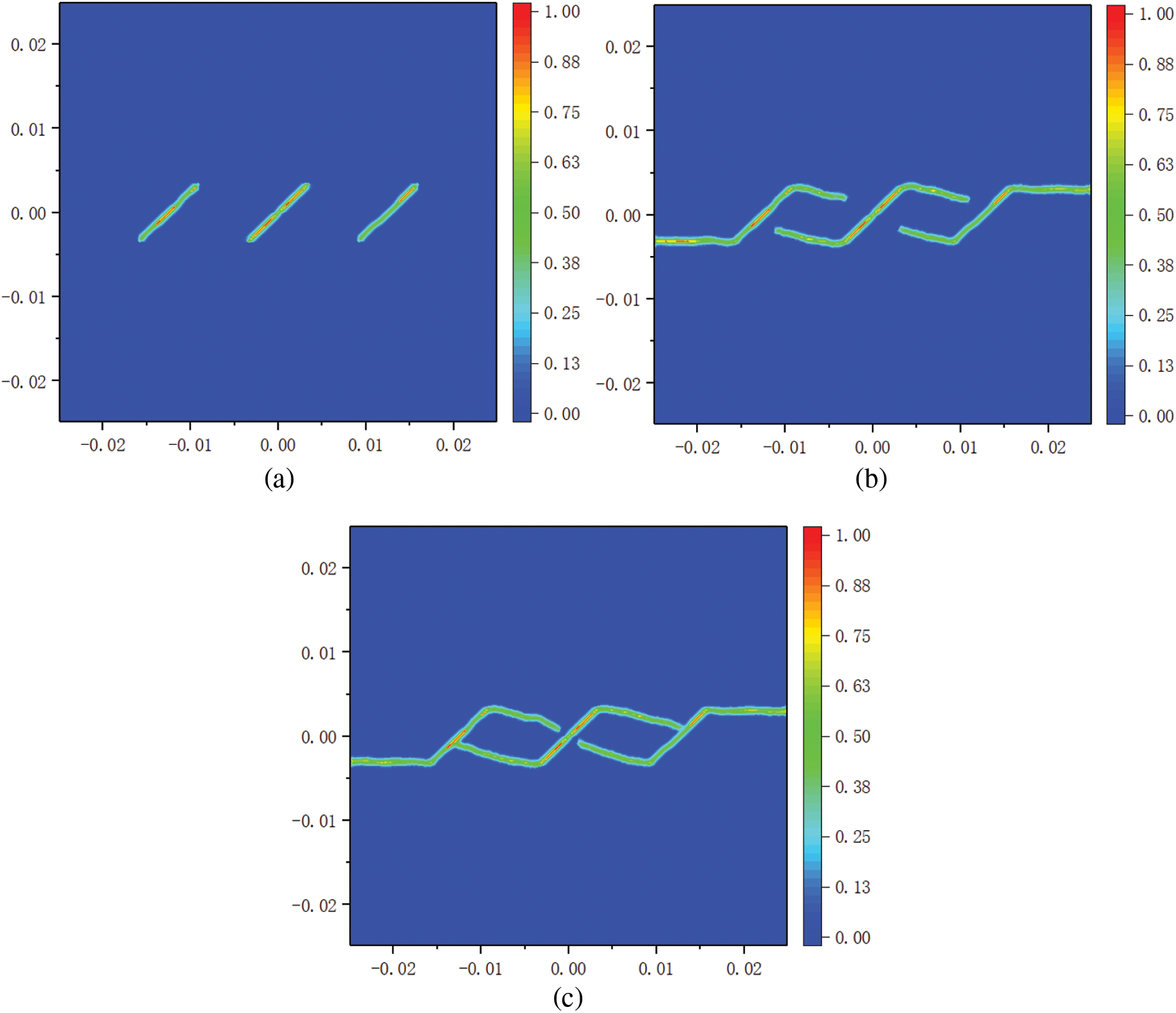
Figure 23: Damage diagram of the cracked plate as shown in Fig. 22a: (a) initiation, (b) propagation, and (c) failure

The propagation of the cracks in Fig. 22b is exhibited in Fig. 24. When the tension on the upper and lower sides reaches 13.5 MPa, three cracks start to propagate at different fracture angles. Before the left end of crack 1 and the right end of crack 2 reach the two vertical edges of the plate, crack 2 extends to firstly connect with crack 1 and crack 3, and then stops cracking. Crack 1 and crack 3 continue to propagate until the left end of crack 1 and the right end of crack 3 reach the boundary of the plate, and the other two ends are linked with crack 2, respectively. Thus, the plate is split into four parts: two large blocks and two small pieces.

Figure 24: Damage diagram of the cracked plate as shown in Fig. 22b: (a) initiation, (b) propagation, and (c) failure

7  Conclusions

By simplification, the transfer functions of the boundary traction are determined. On this basis, the peridynamic motion equation with the boundary traction is improved and used to solve multiple crack propagation in an elastic-brittle square plate subjected to uniaxial tension on the boundary surface. The critical cracking load, fracture angle and propagation path of the crack are investigated. The conclusions are summarized as follows:

1.    The surface correction and artificial boundary layer in the numerical algorithm can be cancelled due to the introduction of the transfer functions of boundary traction.

2.    The brittle fracture can be well characterized by the prototype microelastic model.

3.    The fracture angle can be directly given by peridynamic calculation without relevant criteria.

4.    The fracture mode and propagation path of solids with multiple cracks can be conveniently determined in terms of peridynamics.

Funding Statement: The work was supported by the National Nature Science Foundation of China through the Grant Nos. 12072145 and 11672129.

Conflicts of Interest: The authors declare that they have no conflicts of interest to report regarding the present study.

References

1. Madenci, E., Oterkus, E. (2014). Peridynamic theory and its applications. New York: Springer. [Google Scholar]

2. Silling, S. A. (2000). Reformulation of elasticity theory for discontinuities and long-range forces. Journal of Mechanics and Physics of Solids, 48(1), 175–209. https://doi.org/10.1016/S0022-5096(99)00029-0 [Google Scholar] [CrossRef]

3. Silling, S. A., Askari, E. (2005). A meshfree method based on the peridynamic model of solid mechanics. Computers and Structures, 83(17–18), 1526–1535. https://doi.org/10.1016/j.compstruc.2004.11.026 [Google Scholar] [CrossRef]

4. Le, Q. V., Chan, W. K., Schwartz, J. (2014). A two-dimensional ordinary, state-based peridynamic model for linearly elastic solids. International Journal for Numerical Methods in Engineering, 98(8), 547–561. https://doi.org/10.1002/nme.4642 [Google Scholar] [CrossRef]

5. Silling, S. A., Epton, M., Weckner, O., Xu, J., Askari, E. (2007). Peridynamic states and constitutive modeling. Journal of Elasticity, 88(2), 151–184. https://doi.org/10.1007/s10659-007-9125-1 [Google Scholar] [CrossRef]

6. Wu, C. T., Ren, B. (2015). A stabilized non-ordinary state-based peridynamics for the nonlocal ductile material failure analysis in metal machining process. Computer Methods in Applied Mechanics and Engineering, 291(245–246), 197–215. https://doi.org/10.1016/j.cma.2015.03.003 [Google Scholar] [CrossRef]

7. Bergel, G. L., Li, S. (2016). The total and updated Lagrangian formulation of state-based peridynamics. Computational Mechanics, 58, 351–370. https://doi.org/10.1007/s00466-016-1297-8 [Google Scholar] [CrossRef]

8. Zhao, J., Tan, L., Dou, X. (2021). Crack propagation with different radius local random damage based on peridynamic theory. Frontiers of Structural and Civil Engineering, 15(5), 1238–1248. https://doi.org/10.1007/s11709-021-0695-y [Google Scholar] [CrossRef]

9. Ferté, G., Massin, P., Moës, N. (2016). 3D crack propagation with cohesive elements in the extended finite element method. Computer Methods in Applied Mechanics and Engineering, 300, 347–374. https://doi.org/10.1016/j.cma.2015.11.018 [Google Scholar] [CrossRef]

10. Javili, A., Morasata, R., Oterkus, E., Oterkus, S. (2018). Peridynamics review. Mathematics and Mechanics of Solids, 24(11), 3714–3719. https://doi.org/10.1177/1081286518803411 [Google Scholar] [CrossRef]

11. Silling, S. A., Bobaru, F. (2005). Peridynamic modeling of membranes and fibers. International Journal of Non-Linear Mechanics, 40(2–3), 395–409. https://doi.org/10.1016/j.ijnonlinmec.2004.08.004 [Google Scholar] [CrossRef]

12. Bobaru, F., Yang, M. J., Leonardo, F. A., Silling, S. A. (2009). Convergence, adaptive refinement, and scaling in 1D peridynamics. International Journal for Numerical Methods in Engineering, 77(6), 852–877. https://doi.org/10.1002/nme.2439 [Google Scholar] [CrossRef]

13. Bobaru, F., Zhang, G. F. (2015). Why do cracks branch? A peridynamic investigation of dynamic brittle fracture. International Journal of Fracture, 196(1–2), 59–98. https://doi.org/10.1007/s10704-015-0056-8 [Google Scholar] [CrossRef]

14. Ha, Y. D., Bobaru, F. (2011). Characteristics of dynamic brittle fracture captured with peridynamics. Engineering Fracture Mechanics, 78(5), 1156–1168. https://doi.org/10.1016/j.engfracmech.2010.11.020 [Google Scholar] [CrossRef]

15. Ha, Y. D., Bobaru, F. (2010). Studies of dynamic crack propagation and crack branching with peridynamics. International Journal of Fracture, 162(1–2), 229–244. https://doi.org/10.1007/s10704-010-9442-4 [Google Scholar] [CrossRef]

16. Dipasquale, D., Zccariotto, M., Galvanetto, U. (2014). Crack propagation with adaptive grid refinement in 2D peridynamics. International Journal of Fracture, 192(1–2), 1–22. https://doi.org/10.1007/s10704-014-9970-4 [Google Scholar] [CrossRef]

17. Dipasquale, D., Sarego, G., Zccariotto, M., Galvanetto, U. (2016). Dependence of crack paths on the orientation of regular 2D peridynamic grids. Engineering Fracture Mechanics, 160(2), 248–263. https://doi.org/10.1016/j.engfracmech.2016.03.022 [Google Scholar] [CrossRef]

18. Madenci, E., Colavito, K., Phan, N. (2016). Peridynamics for unguided crack growth prediction under mixed-mode loading. Engineering Fracture Mechanics, 167(2), 33–44. https://doi.org/10.1016/j.engfracmech.2016.04.009 [Google Scholar] [CrossRef]

19. Wang, Y., Zhou, X., Xu, X. (2016). Numerical simulation of propagation and coalescence of flaws in rock materials under compressive loads using the extended non-ordinary state-based peridynamics. Engineering Fracture Mechanics, 163(4), 248–273. https://doi.org/10.1016/j.engfracmech.2016.06.013 [Google Scholar] [CrossRef]

20. Gu, X., Zhang, Q., Xia, X. (2017). Voronoi-based peridynamics and cracking analysis with adaptive refinement. International Journal for Numerical Methods in Engineering, 112(13), 2087–2109. https://doi.org/10.1002/nme.5596 [Google Scholar] [CrossRef]

21. Lee, J., Ha, Y. D., Hong, J. W. (2017). Crack coalescence morphology in rock-type material under compression. International Journal of Fracture, 203(1), 211–236. https://doi.org/10.1007/s10704-016-0138-2 [Google Scholar] [CrossRef]

22. Wang, Y. T., Zhou, X. P., Shou, Y. D. (2017). The modeling of crack propagation and coalescence in rocks under uniaxial compression using the novel conjugated bond-based peridynamics. International Journal of Mechanical Sciences, 128–129(3), 614–643. https://doi.org/10.1016/j.ijmecsci.2017.05.019 [Google Scholar] [CrossRef]

23. Wang, Y. T., Zhou, X. P., Wang, Y., Shou, Y. D. (2017). A 3-D conjugated bond-pair-based peridynamic formulation for initiation and propagation of cracks in brittle solids. International Journal of Solids and Structures, 134(1–2), 89–115. https://doi.org/10.1016/j.ijsolstr.2017.10.022 [Google Scholar] [CrossRef]

24. Rabczuk, T., Ren, H. (2017). A peridynamics formulation for quasi-static fracture and contact in rock. Engineering Geology, 225(1), 42–48. https://doi.org/10.1016/j.enggeo.2017.05.001 [Google Scholar] [CrossRef]

25. Zhang, T., Zhou, X. P. (2019). A modified axisymmetric ordinary state-based peridynamics with shear deformation for elastic and fracture problems in brittle solids. European Journal of Mechanics A-Solids, 77, 103810. https://doi.org/10.1016/j.euromechsol.2019.103810 [Google Scholar] [CrossRef]

26. Ni, T., Zaccariotto, M., Zhu, Q. Z., Galvanetto, U. (2019). Static solution of crack propagation problems in Peridynamics. Computer Methods in Applied Mechanics and Engineering, 346(3), 126–151. https://doi.org/10.1016/j.cma.2018.11.028 [Google Scholar] [CrossRef]

27. Shojaei, A., Mossaiby, F., Zaccariotto, M., Galvanetto, U. (2018). An adaptive multi-grid peridynamic method for dynamic fracture analysis. International Journal of Mechanical Sciences, 144(1), 600–617. https://doi.org/10.1016/j.ijmecsci.2018.06.020 [Google Scholar] [CrossRef]

28. Shou, Y. D., Zhou, X. P., Berto, F. (2019). 3D numerical simulation of initiation, propagation and coalescence of cracks using the extended non-ordinary state-based peridynamics. Theoretical and Applied Fracture Mechanics, 101(7), 254–268. https://doi.org/10.1016/j.tafmec.2019.03.006 [Google Scholar] [CrossRef]

29. Zhou, X. P., Shou, Y. D. (2017). Numerical Simulation of failure of rock-like material subjected to compressive loads using improved peridynamic method. International Journal of Geomechanics, 17(3), 04016086. https://doi.org/10.1061/(ASCE)GM.1943-5622.0000778 [Google Scholar] [CrossRef]

30. Huang, D., Lu, G., Qiao, P. (2015). An improved peridynamic approach for quasi-static elastic deformation and brittle fracture analysis. International Journal of Mechanical Sciences, 94–95(8), 111–122. https://doi.org/10.1016/j.ijmecsci.2015.02.018 [Google Scholar] [CrossRef]

31. Gu, X. B., Zhou, X. P. (2015). The numerical simulation of tensile plate with circular hole using peridynamic theory. Chinese Journal of Solid Mechanics, 36(5), 376–383. https://doi.org/10.1016//j.cnki.cjsm42-1250/o3.2015.05.002 [Google Scholar] [CrossRef]

32. Ni, T., Zhu, Q. Z., Zhao, L., Li, P. F. (2018). Peridynamic simulation of fracture in quasi brittle solids using irregular finite element mesh. Engineering Fracture Mechanics, 188(10), 320–343. https://doi.org/10.1016/j.engfracmech.2017.08.028 [Google Scholar] [CrossRef]

33. Huang, D., Lu, G., Wang, C., Qiao, P. (2015). An extended peridynamic approach for deformation and fracture analysis. Engineering Fracture Mechanics, 141(8), 196–211. https://doi.org/10.1016/j.engfracmech.2015.04.036 [Google Scholar] [CrossRef]

34. Jo, G., Ha, Y. D. (2022). Two-grid based sequential peridynamic analysis method for quasi-static crack propagation. Engineering Fracture Mechanics, 269, 108549. https://doi.org/10.1016/j.engfracmech.2022.108549 [Google Scholar] [CrossRef]

35. Lai, X., Liu, L., Li, S., Zelekea, M., Liu, Q. et al. (2018). A non-ordinary state-based peridynamics modeling of fractures in quasi-brittle materials. International Journal of Impact Engineering, 111, 130–146. [Google Scholar]

36. Zhang, N., Gu, Q., Huang, S., Xue, X., Li, S. (2021). A practical bond-based peridynamic modeling of reinforced concrete structures. Engineering Structures, 244, 112748. [Google Scholar]

37. Song, R., Han, F., Mei, Y., Sun, Y., Zhang, A. (2022). A hybrid local/nonlocal continuum mechanics modeling of damage and fracture in concrete structure at high temperatures. Computer Modeling in Engineering & Sciences, 133(2), 389–412. https://doi.org/10.32604/cmes.2022.021127 [Google Scholar] [CrossRef]

38. Huang, Z. (2019). Revisiting the peridynamic motion equation due to characterization of boundary conditions. Acta Mechanica Sinica, 35(5), 972–980. https://doi.org/10.1007/s10409-019-00860-3 [Google Scholar] [CrossRef]

39. Zhou, K., Du, Q. (2010). Mathematical and numerical analysis of linear peridynamic models with nonlocal boundary conditions. SIAM Journal on Numerical Analysis, 48(5), 1759–1780. https://doi.org/10.1137/090781267 [Google Scholar] [CrossRef]

40. Macek, R. W., Silling, S. A. (2007). Peridynamics via finite element analysis. Finite Elements in Analysis and Design, 43(15), 1169–1178. https://doi.org/10.1016/j.finel.2007.08.012 [Google Scholar] [CrossRef]

41. Bobaru, F., Hu, W. (2012). The meaning, selection, and use of the peridynamic horizon and its relation to crack branching in brittle materials. International Journal of Fracture, 176(2), 215–222. https://doi.org/10.1007/s10704-012-9725-z [Google Scholar] [CrossRef]

42. Silling, S. A., Lehoucq, R. B. (2008). Convergence of peridynamics to classical elasticity theory. Journal of Elasticity, 93(1), 13–37. https://doi.org/10.1007/s10659-008-9163-3 [Google Scholar] [CrossRef]

43. Bobaru, F., Foster, J. T., Geubelle, P. H., Silling, S. A. (2017). Handbook of peridynamic modeling. Boca Raton: CRC Press. [Google Scholar]

44. Liu, W., Hong, J. W. (2012). Discretized peridynamics for linear elastic solids. Computational Mechanics, 50(5), 579–590. https://doi.org/10.1007/s00466-012-0690-1 [Google Scholar] [CrossRef]

45. Parks, M. L., Lehoucq, R. B., Plimpton, S. J., Silling, S. A. (2008). Implementing peridynamics within a molecular dynamics code. Computer Physics Communications, 179(11), 777–783. https://doi.org/10.1016/j.cpc.2008.06.011 [Google Scholar] [CrossRef]

46. Kilic, B., Madenci, E. (2010). An adaptive dynamic relaxation method for quasi-static simulations using the peridynamic theory. Theoretical and Applied Fracture Mechanics, 53(3), 194–201. https://doi.org/10.1016/j.tafmec.2010.08.001 [Google Scholar] [CrossRef]

47. Oterkus, E., Madenci, E., Weckner, O., Silling, S. A., Bogert, P. et al. (2012). Combined finite element and peridynamic analyses for predicting failure in a stiffened composite curved panel with a central slot. Composite Structures, 94(3), 839–850. https://doi.org/10.1016/j.compstruct.2011.07.019 [Google Scholar] [CrossRef]

48. Wu, C. T., Ren, B. (2014). Localized particle boundary condition enforcements for the state based peridynamics. Interaction and Multiscale Mechanics, 7(1), 525–542. https://doi.org/10.12989/imm.2014.7.1.525 [Google Scholar] [CrossRef]

49. Wu, C. T., Hu, W. (2011). Meshfree-enriched simplex elements with strain smoothing for the finite element analysis of compressible and nearly incompressible solids. Computer Methods in Applied Mechanics and Engineering, 200(45–46), 2991–3010. https://doi.org/10.1016/j.cma.2011.06.013 [Google Scholar] [CrossRef]

50. Prudhomme, S., Diehl, P. (2020). On the treatment of boundary conditions for bond-based peridynamic models. Computer Methods in Applied Mechanics and Engineering, 372(1), 113391. https://doi.org/10.1016/j.cma.2020.113391 [Google Scholar] [CrossRef]

51. Scabbia, F., Zaccariotto, M., Galvanetto, U. (2022). A new method based on Taylor expansion and nearest-node strategy to impose Dirichlet and Neumann boundary conditions in ordinary state-based Peridynamics. Computational Mechanics, 70(1), 1–27. https://doi.org/10.1007/s00466-022-02153-2 [Google Scholar] [CrossRef]

52. Liu, Y., Han, F., Zhang, L. (2022). An extended fictitious node method for surface effect correction of bond-based peridynamics. Engineering Analysis with Boundary Elements, 143(1), 78–94. https://doi.org/10.1016/j.enganabound.2022.05.023 [Google Scholar] [CrossRef]

53. Yu, Y., You, H., Trask, N. (2021). An asymptotically compatible treatment of traction loading in linearly elastic peridynamic fracture. Computer Methods in Applied Mechanics and Engineering, 377(1), 113691. https://doi.org/10.1016/j.cma.2021.113691 [Google Scholar] [CrossRef]

54. Zhou, Z., Yu, M., Wang, X., Huang, Z. (2022). Peridynamic analysis of 2-dimensional deformation and fracture based on an improved technique of exerting traction on boundary surface. Archives of Mechanics, 74(6), 441–461. https://doi.org/10.24423/aom.4096 [Google Scholar] [CrossRef]

55. Yu, M., Zhou, Z., Huang, Z. (2023). Traction-associated peridynamic motion equation and its verification in the plane stress and fracture problems. Materials, 16(6), 2252. https://doi.org/10.3390/ma16062252 [Google Scholar] [PubMed] [CrossRef]

56. Silling, S. A., Lehoucq, R. B. (2010). Peridynamic theory of solid mechanics. Advance in Applied Mechanics, 44, 73–168. https://doi.org/10.1016/S0065-2156(10)44002-8 [Google Scholar] [CrossRef]

57. Yu, H., Li, S. (2020). On energy release rates in peridynamics. Journal of Mechanics and Physics of Solids, 142(3), 104024. https://doi.org/10.1016/j.jmps.2020.104024 [Google Scholar] [CrossRef]

58. Mikata, Y. (2012). Analytical solutions of peristatic and peridynamic problems for a 1D infinite rod. International Journal of Solids and Structures, 49(21), 2887–2897. https://doi.org/10.1016/j.ijsolstr.2012.02.012 [Google Scholar] [CrossRef]

59. Silling, S. A., Zimmermann, M., Abeyaratne, R. (2003). Deformation of a peridynamic bar. Journal of Elasticity, 73(1–3), 173–190. https://doi.org/10.1023/B:ELAS.0000029931.03844.4f [Google Scholar] [CrossRef]

60. Cox, J. V. (2009). An extended finite element method with analytical enrichment for cohesive crack modeling. International Journal for Numerical Methods in Engineering, 78(1), 48–83. https://doi.org/10.1002/nme.2475 [Google Scholar] [CrossRef]

61. Rooke, D. P., Cartwright, D. J. (1976). Compendium of stress intensity factors. London: Her Majesty’s Stationery Office. [Google Scholar]